Chapter 4
Application to a chemical reaction process
This chapter summarizes an application of MSPC, described in Chapters 1 to 3, to recorded data from a chemical reaction process, producing solvent chemicals. Data from this process have been studied in the literature using PCA and PLS, for example (Chen and Kruger 2006; Kruger et al. 2001; Kruger and Dimitriadis 2008; Lieftucht et al. 2006a). Sections 4.1 and 4.2 provide a process description and show how to determine a PCA monitoring model, respectively. Finally, Section 4.3 demonstrates how to detect and diagnose a fluidization problem in one of the tubes.
4.1 Process description
This process produces two solvent chemicals, denoted as F and G, and consists of several unit operations. The core elements of this plant are five parallel fluidized bed reactors, each producing F and G by complex exothermic reactions. These reactors are fed with five different reactants. Figure 4.1 shows one of the parallel reactors.
Figure 4.1 Schematic diagram of chemical reaction process.
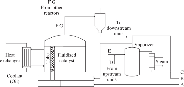
Streams A, B and C represent fresh reactant feed supplying pure components A, B and C, while feedstream D is from an upstream unit. Stream E is plant recycle. Streams D and E are vaporized before entering the reactor. After leaving the reactors, the separation of components F and G is achieved by downstream distillation units.
Each reactor consists of a large shell and a number of vertically oriented tubes in which the chemical reaction is carried out, supported by fluidized catalyst. There is a thermocouple at the bottom of each tube to measure the temperature of the fluidized bed. To remove the heat of the exothermic reaction, oil circulates around the tubes.
The ratio of components F and G is obtained from a lab analysis at eight hour intervals. Based on this analysis, operators adjust the F:G ratio by manipulating reactor feedrates. To keep the catalyst fluidized at all times, the fluidization velocity is maintained constant by adjusting reactor pressure relative to the total flow rate.
The chemical reaction is affected by unmeasured disturbances and changes in the fluidization of the catalyst. The most often observed disturbances relate to pressure upsets in the steam supply to the vaporizer and the coolant, which is provided by a separate unit. Fluidization problems appear if the catalyst density is considerably greater at the bottom of the tube, which additionally enhances chemical reaction in the tube resulting in a significant increase in the tube temperature.
During a period of several weeks, normal operating data as well as data describing abnormal process behavior were recorded for a single reactor. The reference data set had to be selected with care, to ensure that it did not capture disturbances as described above or fluidization problems of one or more tubes. Conversely, if the size of the reference data set was too small then common cause variation describing the reaction system may not be adequately represented.
4.2 Identification of a monitoring model
Since any disturbance leads to alterations in the reacting conditions and hence the tube temperatures, the analysis here is based on the recorded 35 tube temperatures. Thus, the data structure in 2.2 allows modeling of the recorded variables. Figure 4.2 shows time-based plots of the temperature readings for the reference data, recorded at 1 minute intervals.
Figure 4.2 Recorded sequence of reference data for chemical reaction process.
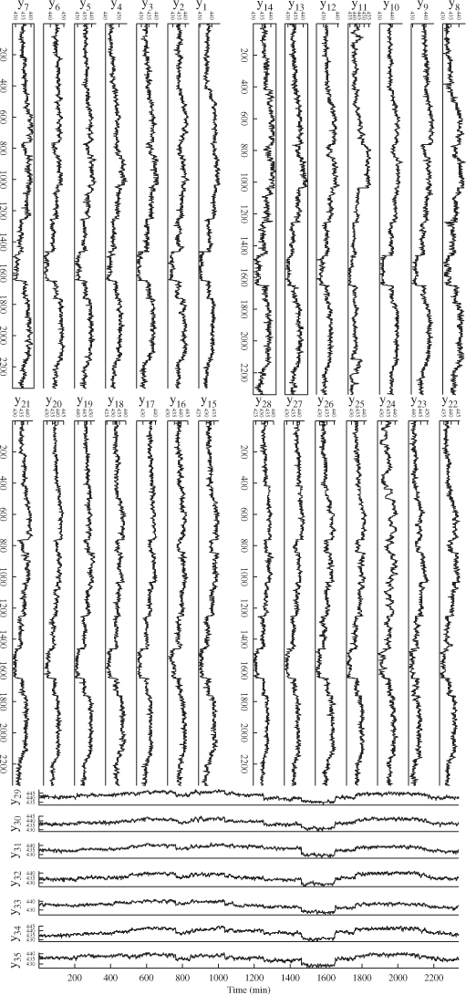
A closer inspection of the 35 variables in Figure 4.2 suggests significant correlation between the tube temperatures, since most of them follow a similar pattern. The identification of a PCA model requires the estimation of the mean vector and the data covariance matrix using 2.13 and 2.14. The mean vector contains values between 330 and 340°C.
Dividing each of the mean-centered signals by its associated standard deviation allows the construction of the correlation matrix. The observation that the tube temperatures are highly correlated can be verified by analyzing the non-diagonal elements of the correlation matrix, ![]() . Displaying the upper left block of this matrix of the first five tube temperatures
. Displaying the upper left block of this matrix of the first five tube temperatures
4.1 
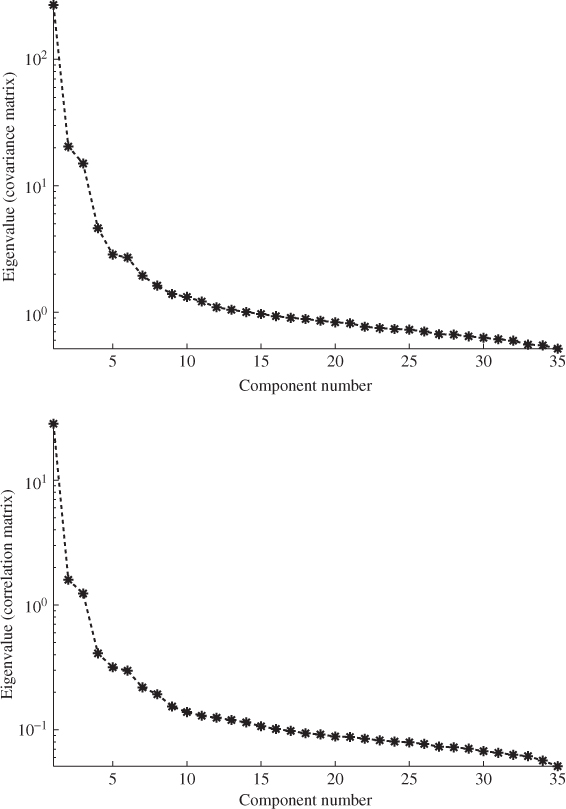
confirms this, as most of the correlation coefficients are larger than 0.8 indicating significant correlation among the variables. Jackson (2003) outlined that it often makes negligible difference which matrix to use for constructing a PCA model in practice. The analysis of the reference data in Figure 4.3 confirm this later on by inspecting the distribution of the eigenvalues for both matrices.
Equation (4.2) shows the upper left block of the covariance matrix
Figure 4.3 plots the distribution of the eigenvalue for the covariance and the correlation matrix and shows that they are almost identical up to a scaling factor.
Figure 4.3 Eigenvalues distribution of data covariance (upper plot) and data correlation matrix (lower plot).
The construction of the covariance matrix is followed by determining the number of source signals. Section 2.4 outlined that the VRE method provides a consistent estimation of n under the assumption that ![]() and is a computationally efficient method. Figure 4.4 shows the results when the covariance and correlation matrices are used. For both matrices, the minimum of the VRE criteria is for four source signals.
and is a computationally efficient method. Figure 4.4 shows the results when the covariance and correlation matrices are used. For both matrices, the minimum of the VRE criteria is for four source signals.
Figure 4.4 Selection of the number of retained PCs using the VRE technique.
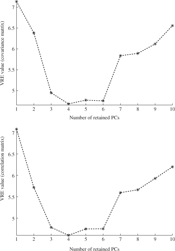
Figure 4.5 shows the time-based plots of these four score variables. With regards to 2.8, these score variables represent linear combinations of the score variables that are corrupted by the error vector. On the other hand, the score variables are the coordinates for the orthogonal projection of the samples onto the model plane according to Figure 2.2 and 2.5.
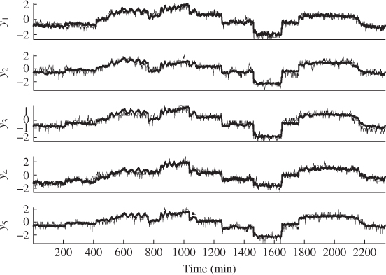
Figure 4.5 Time-based plot of the score variables for reference data.
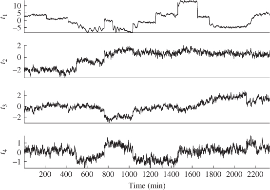
A comparison of the signals in Figure 4.5 with those of Figure 4.2 suggests that the 4 source signals can capture the main variation within the reference data. This can be verified more clearly by comparing the signals of the original tube temperatures with their projections onto the PCA model subspace, which Figure 4.6 illustrates for the first five temperature readings. The thick lines represent the recovered signals and the thin lines correspond to the five recorded signals.
Figure 4.6 Time-based plot of the first five tube temperature readings and their projections onto the PCA model subspace.
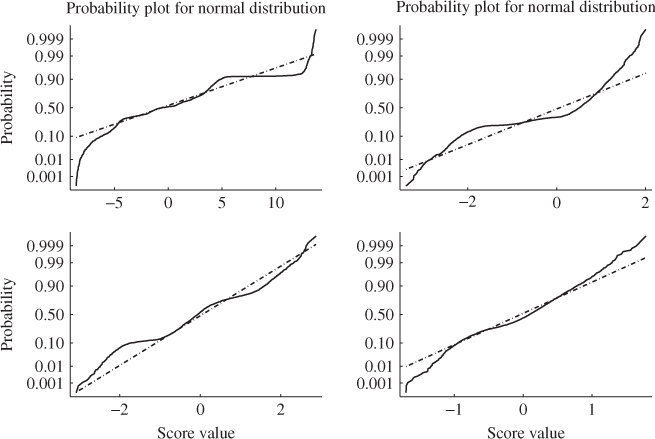
The analysis conducted thus far suggests that the identified data structure models the reference data accurately. By inspecting Figures 4.2 and 4.5, however, the original process variables, and therefore the score variables, do not follow a Gaussian distribution. Figure 4.7 confirms this by comparing the estimated distribution function with that of a Gaussian distribution. The comparison shows very significant departures, particularly for the first two score variables.
Figure 4.7 Comparison between normal distribution (dashed line) and estimated distribution for principal components (solid line).
Theorem 9.3.4 outlines that the score variables are asymptotically Gaussian distributed, which follows from the central limit theorem (CLT). This, however, requires a significant number of variables. Chapter 8 discusses how to address non-Gaussian source signals and in Section 6.1.8 shows that the assumption ![]() is not met. More precisely, it must be assumed that each error variable has a slightly different variance and that the number of source signals is significantly larger than four.
is not met. More precisely, it must be assumed that each error variable has a slightly different variance and that the number of source signals is significantly larger than four.
For the reminder of this section, the statistical inference is based on the assumption that the score variables follow a multivariate Gaussian distribution to demonstrate the working of MSPC for detecting and diagnosing process faults. Chapter 3 highlights that process monitoring relates to the use of scatter diagrams as well as the Hotelling's T2 and Q monitoring statistics.
In relation to Figure 4.7, however, it is imperative to investigate the effect of the non-Gaussian distributed score variables upon both nonnegative quadratic statistics. Figure 4.8 highlights, as expected, significant departures for the T2 statistic, which is assumed to follow and F-distribution with 4 and 2334 degrees of freedom. However, the F-distribution with 31 and 2334 degrees of freedom is a good approximation of the Q statistic when constructed using Equation (3.19).
Figure 4.8 Comparison between F-distribution (dashed line) and estimated distribution for the Hotelling's T2 (upper plot) and Q (lower plot) statistics.
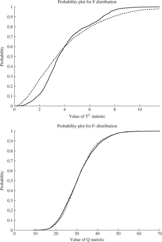
Figure 4.9 plots the resulting Hotelling's T2 and Q statistics for the reference data. The effect of the 4 non-Gaussian source signals upon the Hotelling's T2 statistic can clearly be noticed, as there are no violations of the control limit, which was determined for a significance of 1%. In contrast, the Q statistic violates the control limit a total of 18 times out of 2338, which implies that the number of Type I errors is roughly 1%. This result does not surprise given that the approximation of this statistic is very close to an F-distribution, which the lower plot in Figure 4.8 shows.
Figure 4.9 Time based plot of Hotelling's T2 and Q statistics for reference data.
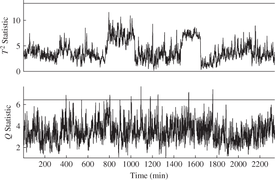
With regards to the Hotelling's T2 statistic, the upper plot in Figure 4.8 gives a clear indication as to why there are no violations. The critical values of the empirical distribution function for α = 0.05 and α = 0.99 are 7.5666 and 8.9825, respectively. However, computing the control limit using 3.5 for a significance of α = 0.01 yields 13.3412. This outlines that the Hotelling's T2 statistic is prone to significant levels of Type II errors and may not be sensitive in detecting incipient fault conditions. The next subsection shows how to use the monitoring model to detect abnormal tube behavior and to identify which of the tube(s) behave anomalously.
It should be noted that the usefulness of applying a multivariate analysis of the recorded data is not restricted to the generation of the Hotelling's T2 and Q statistics. Section 2.1 outlined that the elements of different loading vectors can be plotted against each other. As discussed in Kaspar and Ray (1992), such loading plots can identify groups of variables that have a similar covariance structure and hence show similar time-based patterns of common cause variation that are driven by the source signals. Figure 4.10 shows the loading plot of the first three eigenvectors of ![]() .
.
Figure 4.10 Loading plots of first three eigenvectors of estimated correlation matrix.
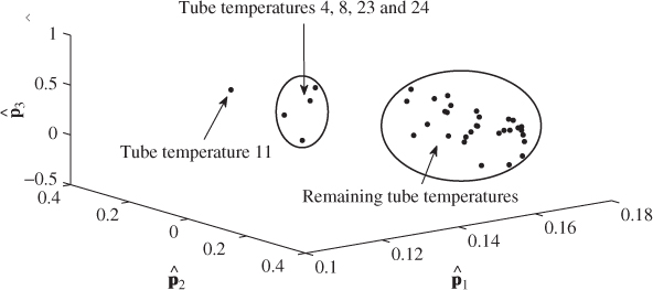
The figure shows that most of the temperature variables fall within a small section, implying that they have very similar patterns on the basis of the first three components. A second and considerably smaller cluster of variables emerges that include the temperature sensors y4, y8, y23 and y24. The analysis also shows that thermocouple #11 (y11) is isolated from the other two clusters. A comparison between the variables that make up the second cluster and thermocouple #11 yields that the signal for y11 shows more distinct operating conditions. In contrast y4, y8, y23 and y24 show substantially more variation and only a few distinct steady state operating regions.
As the thermocouples measure the temperature at the bottom of each tube, the two distinct clusters in Figure 4.10 may be a result of different conditions affecting the chemical reaction within the tubes. This could, for example, be caused by differences in the fluidization of the catalyst or the concentration distribution of the five feeds among the tubes. The distinct behavior of tube #11 would suggest the need to conduct to conduct a further and more detailed analysis. It is interesting to note that this tube showed an abnormal behavior at a later stage and developed a severe fluidization problem. The analysis in Kruger et al. (2001) showed that the tube had to be shut down eventually.
Equation (2.2) is, in fact, a correlation model that assumes that the source signals describe common cause variation as the main contributor to the data covariance matrix. In contrast, the error variables have a minor contribution to this matrix. As the correlation-based model is non-causal, it cannot be concluded that the distinct characteristic of tube #11 relative to the other temperature readings is a precursor or an indication of a fluidization problem. However, the picture presented in Figure 4.10 suggests inspecting the performance of this tube in more detail.
4.3 Diagnosis of a fault condition
After generating a PCA-based monitoring model this section shows how to utilize this model for detecting and diagnosing an abnormal event resulting from a fluidization problem in one of the tubes. There are some manipulations a plant operator can carry out to improve the fluidization and hence bring the tube temperature back to a normal operating level. However, incipient fluidization problems often go undetected by plant operators, as illustrated by this example.
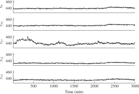
The recorded data showed a total of three cases of abnormal behavior in one of the tubes. Whilst the first two of these events went unnoticed by plant operators, the third one was more severe in nature and required the tube to be shut down (Kruger et al. 2001). The first occurrence is shown in Figure 4.11 by plotting temperature readings #9 to #13 confirming that tube temperature 11 performed abnormally about 100 samples into the data set, which lasts for about 1800 samples (30 hours).
Figure 4.11 Time-based plots of tube temperatures 9 to 13.
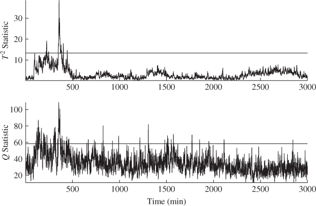
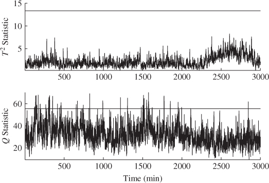
Constructing non-negative quadratic statistics from this data produces the plots displayed in Figure 4.12. The Hotelling's T2 and Q statistics detected this abnormal event about 1 hour and 30 minutes (90 samples) into the data set by a significant number of violations of the Q statistic. The violations covered a period of around 3 hours and 20 minutes (380 samples). The event then decayed in magnitude although significant violations of the Q statistic remained for about 30 hours after which the number of violations were around 1% indicating in-statistical-control behavior.
Figure 4.12 Univariate monitoring statistics representing abnormal tube behavior.
For diagnosing this event, contribution charts are considered first. These include the score variable contribution to the T2 statistic as well as the process variable contribution to the T2 and Q statistics. Figure 4.13 shows these score and variable contributions between the 85th and 92nd samples, which yield that score variables #2 and #4 were predominantly contributing to the T2 statistic. The middle plot shows that the 11th tube temperature was predominantly contributing to the T2 statistic from the 90th sample, which is the first instance where this abnormal event was detected. Furthermore, the variable contribution to the Q statistic does not provide a clear picture although tube temperature 11 was one of the contributing variables among the temperature readings #1, #6, #7, #21 and #34.
Figure 4.13 Contribution charts for samples 85 to 92.
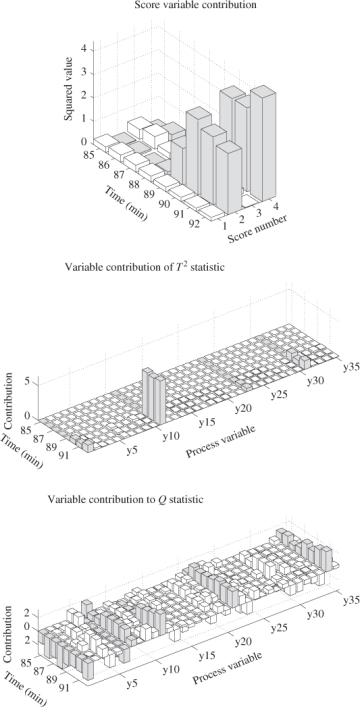
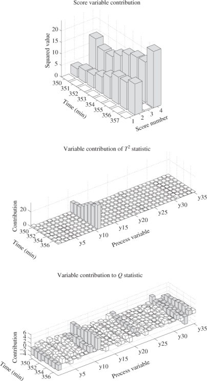
Figure 4.14 presents a second set of contribution charts between the 350th and 357th samples, which covers a period of larger T2 and Q values. As before, score variables #2 and #4 showed a dominant contribution to this event. The middle and lower plots in Figure 4.14 outlined a dominant variable contribution of tube temperature #11 to the T2 and Q statistic, respectively, whilst the lower plot also identified tube temperatures #1, #9, #21, #31, #33 and #34 as affected by this event.
Figure 4.14 Contribution charts for samples 350 to 357.
The above pre-analysis based on contribution charts correctly suggested that tube temperature #11 is the most dominantly affected process variable. Reconstructing this tube temperature using the remaining 34 tube temperatures allows studying the impact of temperature #11 upon the T2 and Q statistics. Subsection 3.2.3 describes how to reconstruct a set of variables using the remaining ones and how to recompute the monitoring statistics to account for the effects of this reconstruction. The reconstruction of tube temperature #11 required the following projection
4.3 
where c11, i are the elements stored in the 11th row of ![]() . To assess the impact of the reconstruction process, Figure 4.14 shows the difference of the eigenvalues for the reconstructed and the original covariance matrix, which are computed as follows
. To assess the impact of the reconstruction process, Figure 4.14 shows the difference of the eigenvalues for the reconstructed and the original covariance matrix, which are computed as follows
4.4 
where ![]() and
and ![]() represent the eigenvalues of
represent the eigenvalues of ![]() and
and ![]() , respectively, and
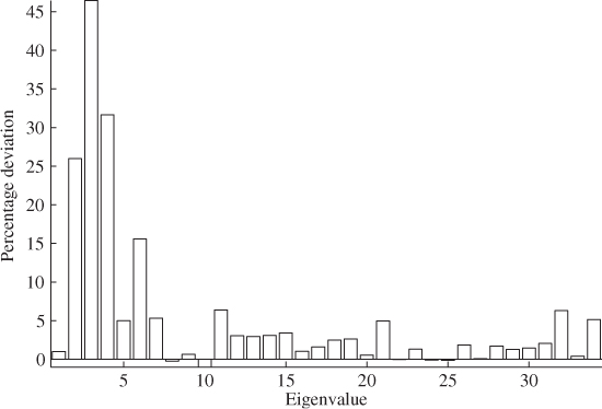
, respectively, and ![]() is the percentage deviation. It follows from Figure 4.15 that the reconstruction of one tube temperature using the remaining ones produced percentage departures of around 5% or less for most eigenvalues. However, eigenvalues #2, #3, #4 and #6 showed departures of up to 45%, which outlines that it is essential to take these changes into account when recalculating the Hotelling's T2 and Q statistics. A detailed discussion of this is given in Subsections 3.2.3 and 3.3.2. Applying the eigenvalues of
is the percentage deviation. It follows from Figure 4.15 that the reconstruction of one tube temperature using the remaining ones produced percentage departures of around 5% or less for most eigenvalues. However, eigenvalues #2, #3, #4 and #6 showed departures of up to 45%, which outlines that it is essential to take these changes into account when recalculating the Hotelling's T2 and Q statistics. A detailed discussion of this is given in Subsections 3.2.3 and 3.3.2. Applying the eigenvalues of ![]() to determine the ‘adapted’ confidence limits yields that:
to determine the ‘adapted’ confidence limits yields that:
- the variances of the score variables changed to 266.4958, 15.1414, 8.0340 and 3.1524 from 269.2496, 20.4535, 14.9976 and 4.6112, respectively; and
- the control limit for the Q statistics changes to 55.0356 from 58.3550.
Figure 4.15 Percentage changes in the eigenvalues of the data covariance matrix for reconstructing tube temperature #11.
The resulting statistics after reconstructing tube temperature #11 are shown in Figure 4.16. Comparing them with those displayed in Figures 4.12 yields that reconstructing temperature reading #11 reduces the number of violations for the Q statistic significantly and removed the violations of the T2 statistic. The remaining violations of the Q statistic are still indicative of an out-of-statistical-control situation. It can be concluded, however, that tube temperature #11 is significantly affected by this event.
Figure 4.16 Univariate monitoring statistics after reconstruction of tube temperature #11.
To control the fluidization of the catalyst, an empirically determined fluidization velocity is monitored and regulated by adjusting the pressure within the reactor. However, the increase in one tube temperature has not been significant enough to show a noticeable effect upon most of the other tube temperatures by this feedback control mechanism, which Figure 4.11 shows. Nevertheless, the controller interaction and hence the changes in pressure within the reactor influenced the reaction conditions, which may contribute to the remaining violations of the Q statistic.
The analysis has so far only indicated that tube temperature #11 is the most dominant contributor to this out-of-statistical-control situation. An estimate of the fault signature and magnitude for each of the tube temperatures, however, could not be offered. Subsection 3.2.3 highlighted that regression-based variable reconstruction can provide such an estimate. Using a total of R = 20 network nodes and a radius of ![]() = 0.1, Figure 4.17 presents the separation of the recorded temperature readings into the fault signature and the stochastic signal components for the first 2000 samples. Given that the abnormal tube behavior did not affect the last 1000 samples, only the first 2000 samples were included in this reconstruction process.
= 0.1, Figure 4.17 presents the separation of the recorded temperature readings into the fault signature and the stochastic signal components for the first 2000 samples. Given that the abnormal tube behavior did not affect the last 1000 samples, only the first 2000 samples were included in this reconstruction process.
Figure 4.17 Estimated fault signature and remaining stochastic signal contribution for tube temperatures #9 to #13.
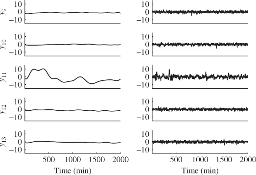
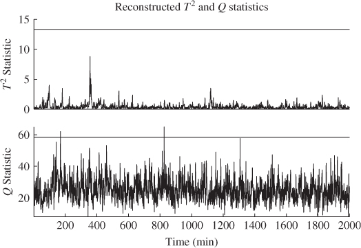
The plots in Figure 4.17 show hardly any contribution from temperature variables #9, #10, #12 and #13 but a substantial fault signature associated with variable #11 that amounts to about 20°C in magnitude. Moreover, apart from very rapid alterations, noticeable by the spikes occurring in the middle left plot in Figure 4.17, the estimated fault signature accurately describes the abnormal tube temperature signal when compared with the original signal in Figure 4.11. Constructing the Hotelling's T2 and Q statistics after the fault signatures have been removed from the recorded temperature readings produced the plots in Figure 4.18. In comparison with Figure 4.16, no statistically significant violations remained.
Figure 4.18 Univariate monitoring statistics after removing the fault signature from the recorded tube temperatures.