
Chapter 9. Control System Concepts
If everything seems under control, you’re just not going fast enough.
A book on real-world data acquisition and control systems would be incomplete without a discussion of the basics of control systems and the theory behind them. Although this chapter is not intended as a detailed or rigorous treatment of control systems, it will hopefully provide enough of a foundation, if you should need it, to enable you to start assembling usable control systems of your own.
Building on the material presented in Chapter 1, this chapter further explores common control system concepts and introduces additional essential details in the form of slightly more formal definitions. It also provides an introduction to basic control system analysis, and gives some guidelines for choosing an appropriate model.
Our primary focus in this chapter will be on simple control systems based on software and electromechanical components. These types of systems would ideally be constructed from readily available instrumentation and control devices such as DMMs, data acquisition units, motor controller modules, power supplies, and power control modules. You shouldn’t have to design and assemble any circuit boards (unless you really want to, of course), or deal with esoteric devices and interfaces—everything you need should be available in an off-the-shelf form. In fact, it might already be on a shelf somewhere gathering dust.
We’ll start off the chapter with an overview of linear, nonlinear, and sequential control systems, followed by definitions of some of the terms and symbols used in control system design. Next, we’ll explore block diagrams and how they are used to diagram control systems. We’ll then take a quick look at the differences between the time and frequency domains, and how these concepts are applied in control systems theory. I won’t go into things like Laplace transfer functions, other than to introduce the concepts, mainly because the types of control systems we’ll be working with can be easily modeled and implemented using garden-variety math.
The next section covers a selection of representative control systems, and shows how the terminology and theory presented in the first section can be applied to them. I’ll present descriptions and examples of open-loop, closed-loop, sequential, PID, nonlinear bang-bang, and hybrid control systems.
To wrap up this chapter, we’ll look at what goes into designing and implementing a control system in Python. We’ll see examples of a proportional control, a nonlinear bang-bang control, and a simple implementation of a proportional-integral-derivative (PID) control.
Basic Control Systems Theory
We are surrounded by control systems, and we ourselves are a form of control system, albeit of a biological nature. A control system may be extremely simple, like a light switch, or very complex, like the autopilot device in an aircraft or the control system in a petrochemical refinery.
Broadly speaking, a control system is any arrangement of components, be they biological, mechanical, pneumatic, electrical, or whatever, that will allow an output action to be regulated or controlled by some form of input. Control systems with the ability to monitor and regulate their own behavior utilize what is called feedback, which is based on the ability to compare the input to the output and generate an error value that is the difference between the two. The error value is used to correct the output as necessary.
A control system isn’t always a single thing in a box by itself. It may contain multiple subsystems, each of which might use a different control paradigm. When assembled together, the subsystems form a cohesive whole with well-defined behavior (ideally, anyway). The overall size of a control system, in terms of its scale and complexity, is a function of its scope. On that basis we could even say that the Earth’s atmosphere is a largely self-regulating climate control and hydraulic distribution system, itself a subsystem of the entire system that is the planet. On a slightly smaller scale, a large ship, like a freighter, is a system for carrying cargo. It contains many subsystems, from the engines and their controls to the helm and the rudder.
If you look around at the various control systems in your immediate environment, you might notice that they are either rather simple or are composed of simple subsystems acting in concert to produce a particular (and perhaps complex) result.
In this chapter we’ll be dealing primarily with three types of control systems: linear, nonlinear, and sequential. A linear control system utilizes a variable control input and produces a variable output as a continuous function of the input. Nonlinear controls, on the other hand, produce a response to a linear input that does not exhibit a continuous relationship with the input. A sequential system, as the name implies, is one that moves through a specific series of states, each of which may produce a specific external output or a subsequent internal state. We won’t be delving into things like fuzzy logic, adaptive controls, or multiple-input/multiple-output control systems. These are deep subject areas in modern control systems research, and they’re way beyond the scope of this book.
Linear Control Systems
As I stated in the introduction to this section, a linear control system produces a variable output as a continuous linear function of the input. For example, consider the following simple equation:
This is the well-known slope intercept equation, and it defines a linear proportional relationship between x and y as a result of m (the slope). The b term applies an optional offset to the output. Could this be used in a control system? Absolutely. In fact, by itself it could be applied as a form of proportional control. Equation 9-1 shows the same equation recast in control system notation.
For discrete-time applications, Equation 9-1 can be written as Equation 9-2.
In Equation 9-2, u(t) is the control output, e(t) is the system error, Kp is the proportional gain applied to the error, and P is the steady-state bias (which could well be zero). The symbol t indicates instantaneous time, otherwise known as “right now.” It doesn’t actually do anything in the equation except to say that the value of u at some time t is a function of the value of e at the same time t.
Don’t worry about what the error is or about the symbols used here for now; we’ll get to them shortly. The important thing to notice is that this is just the slope intercept equation in fancy clothes.
Control systems are typically grouped into two general categories: closed-loop and open-loop. The primary difference between the two involves the ability (or lack thereof) of the system to sense the effect of the controller on the controlled system or device (i.e., its response to the control signal) and adjust its operation accordingly. Closed-loop control systems are also called feedback controllers.
Figure 9-1 shows the response we would expect to see from Equation 9-1. Here I’ve used the error variable as the input, but it’s actually the difference between a reference or control input and the feedback from the device under control (we’ll get into all this in just a bit). The main point here is that it is ideally linear.
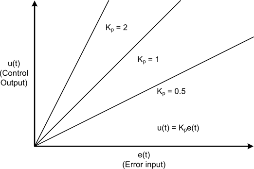
I should point out that while linear models are used extensively in control system analysis and modeling, in reality there are no truly linear systems. For various reasons, every system will exhibit some degree of nonlinear behavior under certain conditions. Also, in a closed-loop feedback system the output response of the controller is dependent on the feedback, and as we will see a little later, feedback from devices with mass, inertia, and time delays can and often do create situations where the resultant graph of the system is not a nice straight line.
Nonlinear Control Systems
A nonlinear control system is one where the input and the output do not have a continuous linear relationship. For example, the output might vary between two (or more) states as a function of a linear input level, as shown in Figure 9-2.
Mathematically, the basic behavior of the system responsible for the graphs in Figure 9-2 can be written in piecewise functional notation, as shown in Equation 9-3.

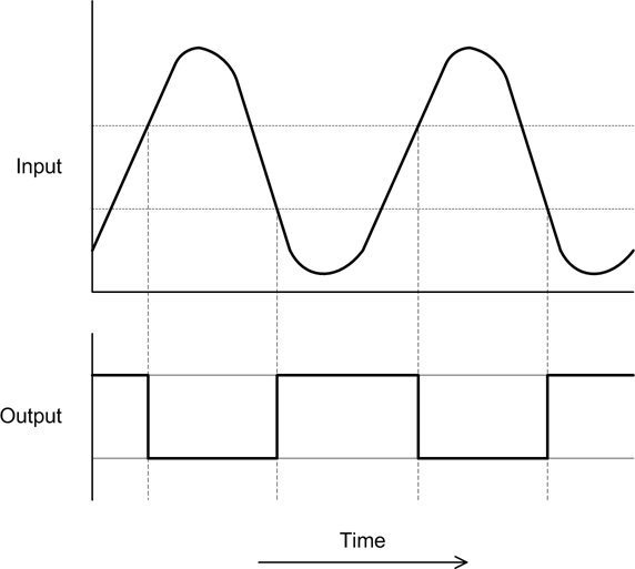
This is typical of the behavior of what is called a bang-bang or on-off type of controller. If the input exceeds a particular high or low limit, the output state changes. Otherwise, it remains in its current state. We’ll take a closer look at this class of controller shortly, and see where it is commonly used in real-life applications.
Now let’s consider a system where a control action occurs for only a specific period of time, like a short burst, and in order to realize a continuous control function both the burst rate and burst duration must be controlled during operation. This is shown in Figure 9-3.
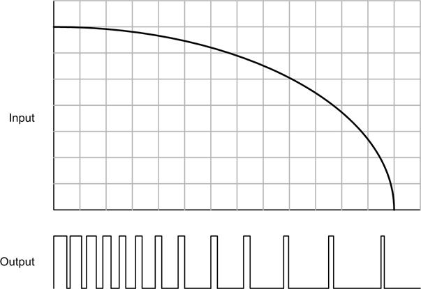
This type of control is found in various applications, such as the antilock braking systems on late-model automobiles, and as the control paradigm for the variable-duty-cycle rocket engines used on robotic planetary landers. In this case the engines are either on or off, and they can only be active for a certain amount of time before they will need to be shut down in order to cool off (otherwise, they will overheat and self-destruct).
Note that the ability to perform continuously variable control of a system is a property of both linear and nonlinear systems. The distinction lies in how the output is manipulated in response to the input in order to achieve control. As we’ll see a little later, the result of a nonlinear control can be a smooth change in the system response, even though the output of the controller itself is definitely not smooth and linear.
Sequential Control Systems
A sequential control system is one wherein the controller has a discrete set of states with inputs and outputs consisting of discrete control signals. The controller might enable or disable devices that themselves utilize discrete states, or they could be linear (or nonlinear) subsystems. The main point is that the devices under control will be either active or inactive, on or off, in a predefined sequence.
Sequential control systems are often found in applications where a series of timed steps are performed in a specific sequence. An example would be an automatic sprinkler system. Internally the sprinkler controller is based on a model composed of sprinkler zones, which typically define groups of commonly plumbed sprinkler heads in certain areas of a yard (or golf course, park, etc.).
Figure 9-4 shows the timing chart for a five-zone sprinkler system. The system is programmed to activate each zone at a certain time on a specific day of the week, and to stay active for some specific duration.
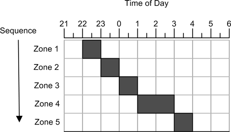
In this example the sequence starts at 2200 hours (10 p.m.) and ends at 0400 (4 a.m.). A typical automatic sprinkler control system is a form of sequential control that relies solely on the current time; it has no other inputs to regulate its behavior. It doesn’t matter if the soil is already damp, or if it is pouring rain; the grass will get watered anyway at the designated times.
Terminology and Symbols
Before we get too much further into control systems, we need to have some terminology to work with, and some symbols to use. Control systems engineering, like any advanced discipline, has its own jargon and symbols. Table 9-1 lists some of the basic terms commonly encountered when dealing with control systems.
Term | Description |
Closed-loop control | A control system that incorporates feedback from the process or plant under control in order to automatically adjust the control action to compensate for perturbations to the system and maintain the intended process output. |
Continuous time | A control system with behavior that is defined at all possible points in time. |
Control signal | Also referred to as the “output.” This is the signal that is applied to a controlled plant or process to make it respond in a desired way. |
Control system | A system with the ability to accept an input and generate an output for the purpose of modifying the behavior of itself or another system. See “System.” |
Controlled output | The response generated by the system as the result of some input and, in a closed-loop control system, the incorporation of feedback into the system. Designated by the letter u in block diagrams. |
Discrete time | A control system with behavior that is defined only at specific points in time. |
Error | The difference between the reference input and the feedback from the plant. |
Feedback | A type of input into the control system that is derived from the controlled plant and compared with the reference input to generate an error value via a summing junction. Designated by the letter b in block diagrams. |
Gain | A multiplier in a system that is used to alter the value of a control or feedback signal. Gain can be changed, but in a conventional control system it is usually not a function of time. In some types of adaptive or nonlinear control systems, gain may be a function of time. |
Input | Also known as the “reference input” when referring to the controller as a whole; otherwise, it can refer to the input of any functional component (block) within the controller. |
Linear control | A control wherein the output is a linear continuous function of the input. |
Nonlinear control | A control wherein the output is not a linear continuous function of the input, but may instead exhibit discrete-state discontinuous behavior as a result of the input. |
Output | Typically refers to the output of a controller or a functional component within the controller, not the plant or process under control (see also “Controlled output”). Designated by the letter c in block diagrams. |
Open-loop control | A control system that does not employ feedback to monitor the effect of the control signal on the plant. An open-loop control system relies primarily on the inherent accuracy and calibration of the control components in the system. |
Plant | An object or system that is to be controlled. Also known as a “process” or a “controlled system,” depending on the type of device or system being controlled. |
Reference input | A stimulus or excitation applied to a control system from some external source. The reference input represents the desired output or behavior of the controlled plant. Designated by the letter r in block diagrams. See also “Input.” |
Sampled data | Data values obtained at specific intervals, each representing the state of a particular signal or system at a discrete point in time. |
Summing node | The point in the control system where the feedback signal is subtracted from the reference input to obtain the error. Can also refer to any point where two or more signals or values are arithmetically combined. |
System | A collection of interconnected functional components that are intended to operate as a unit. |
Some of the alphabetic symbols commonly encountered when working with control system diagrams are listed in Table 9-2.
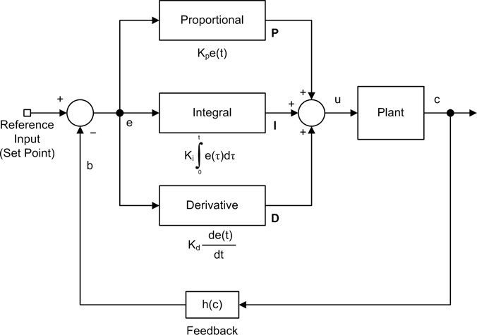
Control System Block Diagrams
Block diagrams are used extensively in control system design and analysis, so I’d like to introduce some of the basic concepts here that we will use throughout the rest of this chapter. Figure 9-5 shows the block diagrams for both an open-loop and a closed-loop control system, along with typical notation for the internal variables.
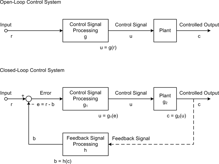
Every control system has at least one input, often called the reference input, and at least one output, referred to as the control signal or the controlled variable. The final output from the plant is called the controlled output, and in a closed-loop system this is what is measured and used as the input to the feedback path. The relationship between the input and the controlled output defines the behavior of the system. In Figure 9-5, the reference input is denoted by the symbol r, the control signal is u, and the controlled output is c. The symbols are historical and still in common use, so I’ll use them here as well.
Input-output relationships
The blocks in a block diagram define processing functions, and each has an input and an output. There may also be auxiliary input variables for things such as bias or external disturbances.
The output may or may not be equal to the response implied by the input. Actually, it is common to find some kind of math going on between the input and the output of a block, which in Figure 9-5 is indicated by the block labeled “Control Signal Processing.” Notice that this block has a symbol for its internal function, which in this case is g (or g1 in the closed-loop system). This might be as simple as multiplication (gain), or perhaps addition (offset). It can also involve integration, differentials, and other operations. It all depends on how the control signal needs to respond to the input in order for the system to perform its intended function.
Feedback
In a closed-loop control system, the control signal is generated from the error signal that is the result of the difference (or sum) of the input and the feedback. The symbol for the feedback signal is b, and it is generated by the function h(c), where c is the feedback signal obtained from the output of the controlled plant. The circle symbol is called the summing node, or summing junction. In Figure 9-5 the b input to the summing node has a negative symbol, indicating that this is a negative feedback system. It is possible, however, to have a positive feedback system, in which case the symbol would be a plus sign.
Transfer Functions
The relationship between the input and the output of a system is typically described in terms of what is called a transfer function. Every block in a control system block diagram can denote a transfer function of some sort, and the overall system-level input/output relationship is determined by the cumulative effects of all of the internal transfer functions. One of the activities that might occur during the design and analysis of a control system is the simplification of the internal transfer functions into a single overall transfer function that describes the end-to-end behavior of the system.
Mathematically, a transfer function is a representation of the relationship between the input and output of a time-invariant system. What does that mean? We’ll get to the definition of time-invariant shortly, but for now what this is saying is that transfer functions are applied in the frequency domain and that the functional relationship does not depend directly on time, just frequency.
In control systems theory the transfer functions are derived using the Laplace transform, which is an integral transform that is similar to the Fourier transform. The primary difference is that the Fourier transform resolves a signal or function into its component frequencies, whereas the Laplace transform resolves it into its “moments.” In control systems theory the Laplace transform is often employed as a transformation from the time domain to the frequency domain. When working with complex or frequency-sensitive systems, the Laplace forms of the transfer functions are usually much easier to deal with and help to simplify the system model.
Although Laplace transforms are widely used, their use is not mandatory. In this chapter I won’t be using Laplace transforms, mainly because much of what we’ll be doing is very straightforward, and also because we will be working almost exclusively in the time domain with systems that are slow enough to not have significant issues with frequency response. For our purposes, basic algebra and calculus will serve just fine.
Time and Frequency
Time and frequency are key components in control system design. Activities occur for specific periods of time, events might occur at some set rate or at varying rates, and AC signals have a particular frequency (or a number of frequencies, in complex signals). The processing operations within a digital control system also require a finite amount of time, and this too must be accounted for in the system design.
Time and frequency domains
When discussing things such as mathematical functions or electrical signals with respect to time, we are dealing with what is called the time domain. If, on the other hand, our main concern is analyzing and processing AC signals in terms of frequency, we will be working in the frequency domain. The two terms refer to how one might perform the mathematical analysis and modeling of a function within a system, and which one is more appropriate depends on what one is looking for as a result of the analysis.
These distinctions may apply to an entire system, but they are more commonly applied to specific subfunctions within a system. For example, a clock or timing subsystem operates in the time domain, whereas a filter or phase-shifting subsystem operates in the frequency domain.
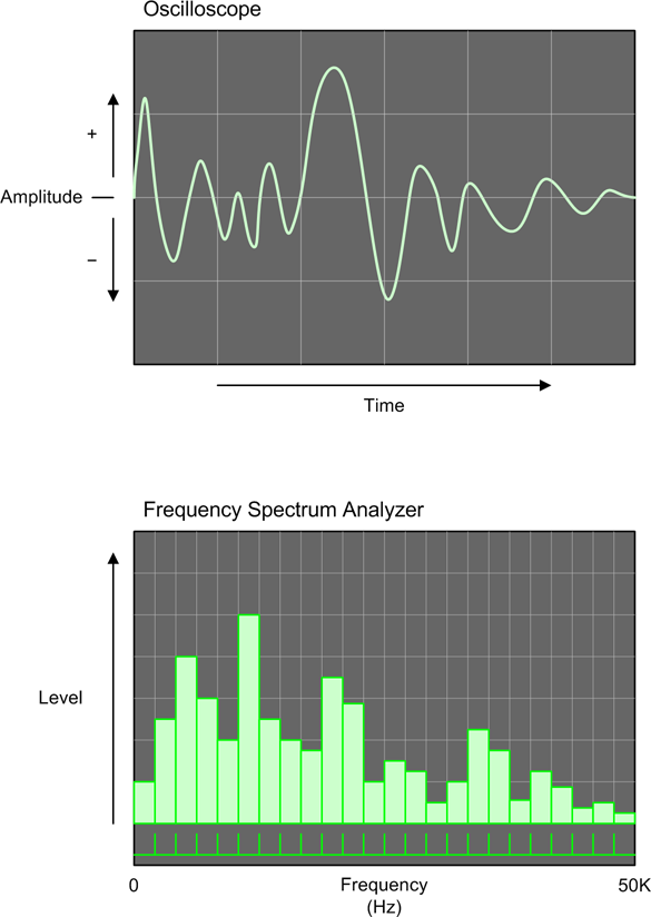
One way to think of the distinction between the time and frequency domains is to consider how you might go about graphing variable data in each domain. Figure 9-6 illustrates what one might expect to see on the displays of an oscilloscope (which we discussed briefly in Chapter 6) and a frequency spectrum analyzer (FSA).
The important point here is that the oscilloscope operates in the time domain, and the FSA operates in the frequency domain. The key is what is being used for the x-axis of the display. With the oscilloscope, the x-axis of the display is time and the y-axis is the amplitude of the signal at any given point along the x-axis. An oscilloscope can be used to determine the time interval between waveforms and the amplitude of the waveforms, but it can’t directly tell you how the component frequencies are distributed within the signal. For that, you’ll need to use the FSA.
The x-axis of the FSA display is frequency, and in Figure 9-6 it ranges from 0 to 50 KHz. I’ve shown the display as a vertical bar graph, but there are other ways to generate the graph. The FSA works by extracting the component frequencies from a signal (perhaps using a set of discrete filters, or by processing the signal using a Fourier analysis technique). The result is a set of values representing the relative amplitudes of the component frequencies within the signal.
We can move back and forth between domains as needed, because time and frequency are just the inverse of one another. It all depends on your perspective. So, given a signal with a period of 20 ms between waveforms, its frequency would be the inverse, or 50 Hz. In other words:
and:
Another example might be a system where pulses from some type of sensor are arriving every 500 μs. If we take the inverse of 0.0005 we get 2,000 Hz, or 2 KHz. This is important to know if we’re thinking of using a data acquisition device with an upper input frequency limit of 1 KHz.
Time and control systems behavior
The behavior of a control system over time is determined by how time affects its operation. The terms time-invariant and time-variant are used to categorize a system’s sensitivity to time.
A time-invariant system is one wherein the output does not depend explicitly on time, and the relationship yt0 = f(xt0) at time t0 will produce the same value for y as the relationship yt1 = f(xt1) at time t1. In other words, the value of y will always be the same for any given value of x regardless of the time.
Time-invariant systems, and particularly linear systems (referred to as linear time-invariant systems, or LTIs), operate primarily in the frequency domain. Each has an input/output relationship that is given by the Fourier transform of the input and the system’s transfer function. An amplifier is an example of an LTI. It doesn’t matter what time it is when a signal arrives at the input; it will be processed according to its frequency and the transfer function embodied in the circuitry, and for any given signal an ideal amplifier will always produce the same output.
A time-variant system is one that is explicitly dependent on time. Time, in this sense, may also be a component of velocity (recall that velocity = distance/time), so a system that is moving is a time-variant system. For example, the autopilot and flight management systems in an aircraft must take time and airspeed into account in order to determine the aircraft’s approximate position as a function of both its velocity and its heading. All of these factors are dependent on time.
Discrete-time control systems
Lastly, we come to discrete-time control systems. This class of control system may be linear or nonlinear, and it is this type of control that we will be working with directly when we’re not using a sequential control scheme. Virtually all control systems that incorporate a computer and software to implement the control and signal processing are discrete-time systems.
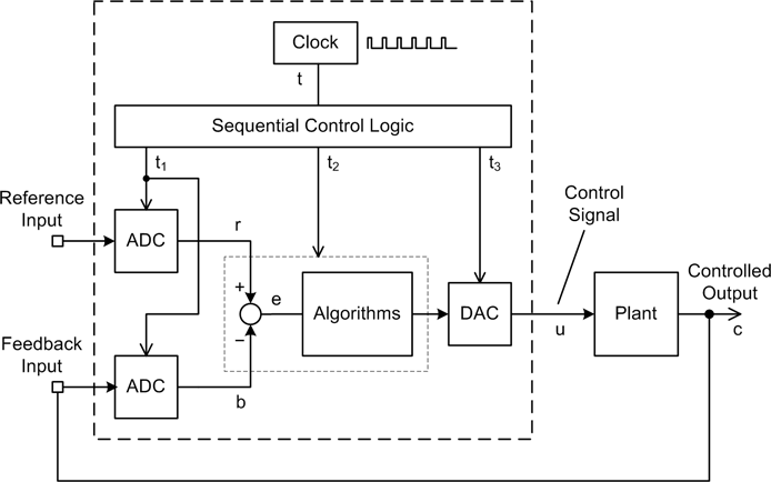
In a traditional analog control system, the relationship between the input and output is immediate and continuous—a change in the input or the feedback is immediately reflected in the output. In a discrete linear control system, the input data acquisition (both reference and error), control processing, and output processing occur in discrete steps governed by a clock, within either a computer or some other type of digital control circuitry. To illustrate this, Figure 9-7 shows the block diagram of a discrete-time closed-loop control system.
In Figure 9-7, the block labeled “Clock” drives some sequential control logic. This could be a microprocessor, or it could be some software. This, in turn, activates the input, processing, and output functions in sequence, as indicated by the signals labeled t1, t2, and t3. It is important to note that just because this is a discrete-time system does not mean that it is also a time-variant system. In this case, any given set of values for r and b at any time t will produce the same values for u and c that would be produced at time t + n, given the same input conditions. It is a discrete-time LTI control.
Note
There is a technique for modeling and analyzing discrete-time systems, referred as the z-transform. This is similar in application to the Laplace transforms used with systems in the continuous domain. When a system contains a mix of both continuous and discrete components, it is not uncommon to map from one domain to the other as necessary for the analysis. We won’t be getting into z-transforms in this book, but I wanted you to be aware of them. What we will be concerned with is discrete system timing and how it can affect a control system’s responsiveness.
In a discrete-time control system, when data is acquired and when control outputs are generated or updated is a function of the overall time required for the controller to complete a full cycle of input, processing, and output activities.
The system under control also has an element of time in the form of a system time constant. The system time constant is the amount of time required for a change to occur over some specific range. In other words, small changes (such as noise) may not be of any concern, but large changes need to be sensed and controlled. How often the control system will need to go through a complete control cycle is a function of the time constant of the system it is controlling.
Figure 9-8 shows a simplified block diagram of the primary software functions in a computer control system, which is composed of the three key functions from Figure 9-7: ADC data acquisition (the “Acquire” block), data-processing algorithms (the “Process” block), and DAC control output (the “Control” block). In the discrete-time environment of the computer these steps occur in a fixed order, and each requires a specific amount of time to execute (as indicated by ta, tp, and to).
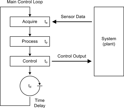
There is also a circular symbol that stands for a time delay of duration td. After the output has been generated, the delay allows the external system to respond before the process is repeated and new control outputs are generated. The delay time would typically be “tuned” to accommodate the time constant of the system it is controlling.
Also notice that the diagram shows an endless loop. This is typical of computer programs for instrumentation applications. Once the steps required for the application have been defined and implemented, the resulting control program runs in a loop, repeating the acquire/process/control steps until either the loop or the entire application is terminated.
Figure 9-9 shows a timing chart representation of the block diagram in Figure 9-8. Here we can see that each activity consumes a specific amount of time. When the line is up, the step is active, and when it’s down, that step is inactive.
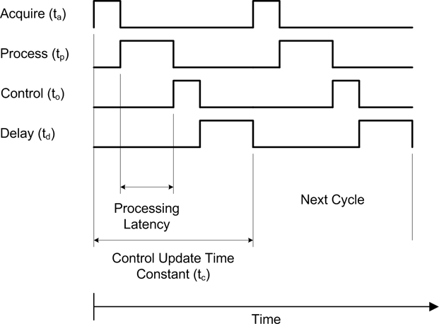
In Figure 9-9 the fundamental time constant for the control system, or the control cycle time, is equivalent to the interval between acquire events. From Figure 9-9 we can see that:
This may seem like a trivial equation, but as we will soon see, the values assigned to these variables can have some profound effects on the system under control. In many cases the delay will contribute the most to the overall control cycle time, although the acquisition time can also be a major factor if external devices are slow in responding.
Control System Types
Up to this point we’ve seen only the basic outline of the domain of things called control systems. In this section we’ll take a look at some specific examples, and apply some of the concepts and terminology. We’ll start by examining examples of open-loop systems, then move on to closed-loop controls, sequential controls, and nonlinear controls. Ultimately we’ll end up at proportional-integral-derivative (PID) controls, the most common form of closed-loop linear control in use today.
Open-Loop Control
In Chapter 1, an automatic outdoor light was used as an example of a nonlinear open-loop system. Linear and nonlinear open-loop control systems operate on the basis of a specific relationship between a control input and the resulting output, and as we’ve already seen, an open-loop controller has no direct “knowledge” of what the actual system is doing in the form of feedback. The accuracy and repeatability of the input/output control relationship is solely dependent on the initial accuracy and calibration of the components in the system.
A gas stove is a familiar example of the input/output relationship in an open-loop control system. The amount of heat applied to a frying pan is determined by the gas control valve on the front of the range top (the control input), and the gas pressure at the valve might be limited by a pressure regulator somewhere in the line (usually at the gas meter outside the house). Once the burner is lit it will produce a flame with an intensity proportional to how the valve is set, but it cannot determine when the pan reaches some specific temperature and regulate the flame accordingly. Some older stoves cannot even determine if the burner is actually lit, and will readily spew raw gas into the kitchen (which is why natural gas has an odor added to it before it is piped to the customer). It is a linear relationship, more or less, but it is a purely open-loop relationship. If the operator (i.e., the cook) sets the flame too high, the scrambled eggs might get a bit too crunchy or the pasta will get scorched. The stove will burn the food just as readily as it will cook it to perfection.
Open-loop controls are useful for applications where the relationship between the input and the output is well defined, and where feedback is not critical for acceptable operation under nominal conditions. However, an open-loop control system cannot respond to continuously changing conditions in the system under control, nor can it deal with transient disturbances or errors. Manual intervention is necessary to adjust the operation of the system as conditions change.
Closed-Loop Control
A closed-loop controller employs feedback to achieve dynamic automatic system control. Closed-loop control systems are also known as feedback control systems, and they may be linear, nonlinear, or even sequential.
Controlling position—Basic feedback
In a closed-loop feedback control system, one or more sensors monitor the output and feed that data back into the system to affect the operation of the controlled system, or plant. In a system that employs negative feedback the objective of the controller is to reduce the error from the summing node to zero (recall the closed-loop part of Figure 9-5).
For example, Figure 9-10 shows the water tank control system from Chapter 1.

In this system time is irrelevant and the functionality is for the most part linear, so it’s an LTI-type system. As with the other examples in this chapter, it is assumed that the control times are slow enough that the frequency response of the system is not a significant concern. The level control setting and the level sensor feedback are the sole inputs to the pump controller.
Let’s take a closer look at this seemingly simple linear system. Figure 9-11 shows the system in block diagram form, and Figure 9-12 shows a pair of graphs depicting the behavior of the pump in response to changes in the water level.
The system block diagram includes additional details such as amplifiers with adjustable gain inputs and an AC power controller for the motor. Since this is a proportional control system, the amount of gain applied to the amplifiers will determine the responsiveness of the system (recall Figure 9-1). The gain variables Km and Kf have a cumulative effect on the system. With the gains set too low, the system will not be able to command the pump to run fast enough to keep up with outflow from the tank. With the gains set too high, the water level will tend to overshoot the target level. In this system, Km is the master gain and Kf is the feedback gain.
The upper graph in Figure 9-12 shows how the level changes as water is drawn off from the tank. The lower graph depicts the behavior of the pump motor in response to a change in the water level. There is a direct inverse linear relationship between the water level and the pump speed.
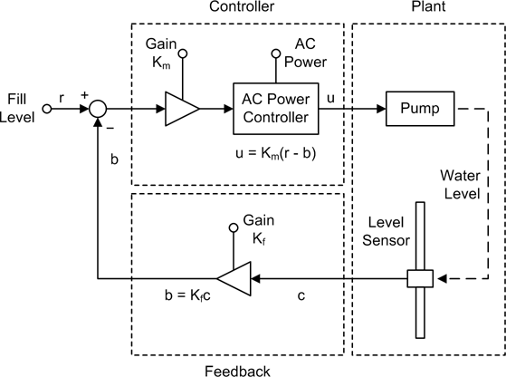

This is a positional control system, with the position in question being that of the float in the tank. When the water level has reached or exceeded a target position, the pump is disabled. When the float is lower than the target water level, the pump is active. In other words, the whole point of this system is to control the position of the float. The pump motor just happens to be the mechanism used to achieve that objective by changing the water level.
Of course, these graphs are just approximations. In a real system you could expect to see things like a small lag between a change in the error value and the motor response. There might also be some overshoot in the water level, and if there was a slow but steady outflow from the tank the level might tend to oscillate around the fill set-point. These and other issues can be addressed by incorporating things like a deadband, time delays, and signal filters into the controller. The gain settings can also play a major role. Adjusting the gain levels in a control system for optimal performance is referred to as tuning, and while it probably wouldn’t be too difficult with a system like this, with other types of control systems it can be a challenge.
Controlling velocity—Feed-forward and PWM controllers
When dealing with systems that involve velocity or speed, the basic closed-loop control won’t quite do the job without some modifications. The reason is that in a system like the water tank (Figure 9-11) the objective is to control the position of the water level in the tank by controlling the position of the float. Once the float has reached the commanded position, the error goes to zero and the control action stops (ideally).
If we want to control the speed of a device like a DC motor, the control system must control the voltage input to the motor to maintain a constant output shaft speed, possibly while handling varying load conditions. Obviously, some kind of feedback is necessary to achieve this, but first consider Figure 9-13, which shows a simple open-loop DC motor control.
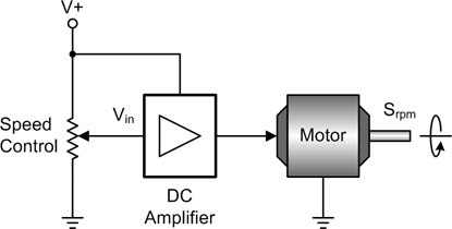
This is a linear control, meaning that the voltage supplied to the motor is a linear function of the voltage at the input of the DC amplifier (Vin), and the shaft speed Srpm is proportional to the input voltage to the motor. The amplifier is an essential component because a typical potentiometer won’t handle the current that a DC motor can draw, and it can also provide gain if needed.
In its simplest form, the equation for Figure 9-13 would be:
where:
- Srpm
Is the motor output RPM
- Mr
Is the motor’s response coefficient
- G
Is the gain of the amplifier
- Vin
Is the input to the amplifier
In the open-loop motor control equation, the Mr coefficient indicates that there are some other factors involving the motor itself. These include the electrical characteristics of the motor as a function of load and shaft RPM, but for our purposes we can lump all these into Mr.
If we want to be able to set the motor speed and then have the system maintain that speed, some type of feedback is required. Assuming that we have some kind of tachometer on the motor shaft that produces a voltage proportional to the motor’s speed, we can use that as the input to the feedback loop.
An arrangement like the closed-loop control shown earlier in Figure 9-11 can be made to work, but it would require some tweaking in terms of the gain values for r, b, and e. Stability is also an issue, and any changes in the load on the motor may result in oscillations in the shaft output speed. Depending on how the various gains are set, the oscillations may take a while to die out.
Another solution is to incorporate a feed-forward path in the control system along with the ability to sense the load on the motor. In a feed-forward type of controller, a control value is passed directly to the controlled device, which then responds in some deterministic and predictable way. Does that sound familiar? It should. Feed-forward is essentially an open-loop control scheme like the one shown in Figure 9-13. In fact, another name for feed-forward is open loop.
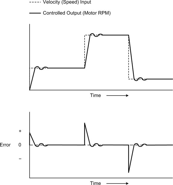
To implement a stable velocity control system, we can add one or more feedback loops for load compensation and speed stability, and use these to adjust the motor’s operation by summing them with the feed-forward input. This arrangement is shown in Figure 9-14. Here, the feedback from a DC tachometer (essentially, a small DC generator) is used to provide stability. The feed-forward input is summed with the velocity error and feedback from a current sensor to compensate for changing torque loads on the motor.
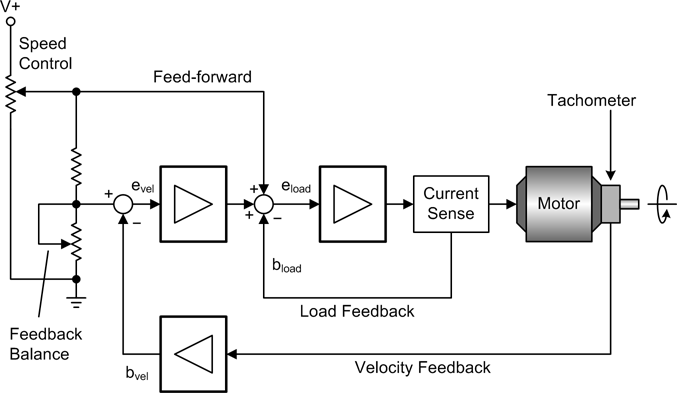
The velocity error bvel will converge to zero so long as the motor’s output RPM matches the reference input. Notice that the reference input is proportional to the speed input. If the load on the motor should change, bload will act to compensate by adjusting the voltage to the motor to hold the speed constant (a motor with no load draws less current at a given RPM than one with a heavy load). Figure 9-15 shows how the error value evel acts to help stabilize the system.
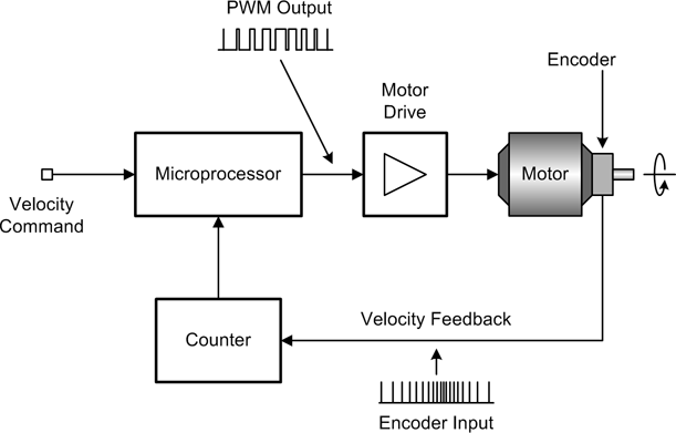
Another way to achieve velocity control is to use pulses for both the motor control and the velocity feedback, as shown in Figure 9-16. For motor velocity control, a pulse-width modulation (PWM) type of control offers better electrical efficiency than a variable voltage controller. A PWM control is also simpler to implement and doesn’t require a DAC component to generate the control signal. A pulse-type encoder that emits one, two, or even four pulses per shaft revolution can be used to determine the rotation speed of a motor’s output shaft by counting the number of pulses that occur within a specific time period. As with the PWM output, this is electrically simple, but notice that a controller of this type, while capable of continuously variable control, is a nonlinear controller. As such, it is heavily dependent on internal processing to read the encoder input, determine the output RPM of the motor, and then modulate the PWM input to the motor to maintain velocity control. The end result is much like what is shown in Figure 9-3.
I’ve shown what is involved in a basic motor control so you will have an idea of what goes into one. These types of controllers are typically implemented as electronic circuits or microcontroller-based modules. Should you encounter a need to control the speed of a motor, I would suggest purchasing a commercial motor speed control unit. Figure 9-17 shows a block diagram with a commercial motor control module.
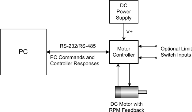
The commands sent to the motor controller in Figure 9-17 would, of course, be in whatever format the manufacturer designed into the controller. In general, a motor controller that accepts ASCII strings will use one character per parameter (direction, velocity, time, and so on), along with the appropriate numeric data for each parameter. The use of RS-232 or RS-485 interfaces for communication with the controller is common, although there are some motor controllers available that are sold as plug-in cards with bus interfaces.
Nonlinear Control: Bang-Bang Controllers
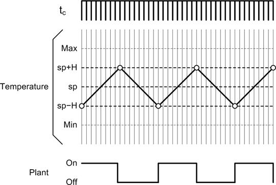
Bang-bang controllers, also known as on-off controllers, are a very common and simple type of nonlinear control system. Bang-bang controllers are so named because the control output responds to a linear input by being either on or off, all or nothing. In pre-electronic times this type of control might have been built with a control arm moving between two mechanical stops, which would result in a “bang” each time the arm moved from the off position to the on position, or vice versa. The thermostat for a typical residential heating and air conditioning system is the control for a closed-loop bang-bang control system. The automatic floodlight we looked at in Chapter 1 is an example of an open-loop bang-bang control system.
Nonlinear control systems often incorporate a characteristic referred to as hysteresis—in effect, a delay between a change in a control input and the response of the system under control. The delay can apply to both “ON” actions and “OFF” actions. In mechanical terms, one can think of it as a “snap action.” A common example of mechanical hysteresis can be found in a typical three-ring notebook, with rings that suddenly open with a “snap” when pulled apart with some amount of force, and then close with a similar snap when moved back together. If the rings simply opened or closed as soon as any force was applied, they would be useless.
In a bang-bang controller, hysteresis is useful for moderating the control action. Figure 9-18 shows the hysteresis found in a common thermostat for an air conditioning unit. It also shows what would happen if there was no built-in hysteresis in the thermostat: the rapid cycling of the air conditioner would soon wear it out.

Because of the hysteresis shown in Figure 9-18, the air conditioner won’t come on until the temperature is slightly higher than the set-point, and it will remain on until the temperature is slightly below the set-point. While this does mean that the temperature will swing over some range around the set-point, it also means that the unit will not continuously and rapidly cycle on and off. Without hysteresis the thermostat would attempt to maintain the temperature at the set-point, which it would do by rapidly cycling the power to the air conditioner. Generally, this is not a good thing to do to a compressor in a refrigeration system.
Electromechanical bang-bang controllers are simple, robust devices that rely mainly on hysteresis in the controller mechanism to achieve a suitable level of responsiveness. However, if a bang-bang control is implemented in software as a discrete-time control system, the various time constants in the software will play a major role in determining how the system responds to input changes and how well it maintains control.
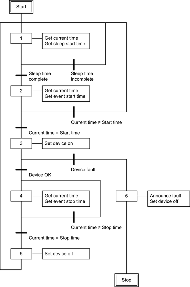
The flowchart in Figure 9-19 shows a simple controller for an air conditioning system. In this implementation hysteresis is determined by the offset constant H, which is applied to the set-point variable s. If the sensed temperature (t) is above or below the set-point with the hysteresis offset applied, the A/C unit will be either powered on or powered off, respectively.
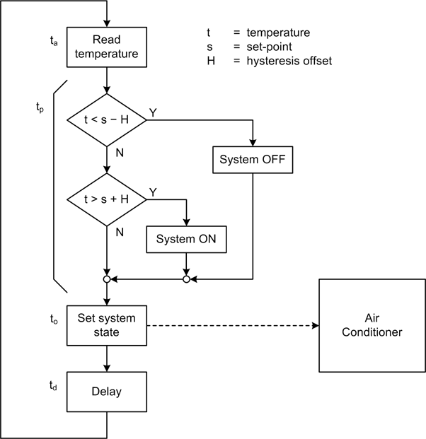
If we refer back to Figure 9-9 and examine Figure 9-19, we can see that in the overall scheme of things, times ta, tp, and to in this system should be negligible. What really counts here is the controller’s cycle time, tc, which is largely composed of the delay time, td.
The control cycle time should be as short as possible (the meaning of short is relative to the system under control, and could well be on the order of many milliseconds). This is a discrete-time control, so it will not have the continuous input response that we would expect from an electromechanical or analog electronic controller. The input needs to be sampled fast enough to avoid situations where the controlled output will overshoot or undershoot the set-point by excessive amounts. With a high sampling rate, the hysteresis coefficient becomes the dominating factor in determining the controlled-output duty cycle.
When determining the optimal value for tc, one must take into account the responsiveness of the system being instrumented. Figure 9-20 shows the idealized response of a bang-bang controller with a relatively high control-sampling rate. The timing for ta, tp, and to is not shown, but we can assume that it’s only a small fraction of tc.
The controller’s cycle time and the amount of hysteresis in the system interact to determine the overall control responsiveness of a discrete-time bang-bang controller. In real applications, a bang-bang controller shouldn’t be used where changes occur rapidly, because the controller will be unable to track the changes. If the time interval between ta and to becomes large relative to the rate of change in the controlled system, the controlled output may continue to change significantly during that time. This can result in overshoot and undershoot, possibly exceeding allowable limits.
Sequential Control Systems
Sequential control systems are typically straightforward to implement, and they can range in complexity from very simple to extremely complex. They are commonly encountered in applications where a specific sequence of actions must be performed to achieve a deterministic result. Earlier, we looked at a simple example of a sequential control system in the form of an automated sprinkler system. Now I’d like to examine a slightly more complex and more interesting example.
Figure 9-21 shows a sequentially controlled robotic device. Here we have a mechanism consisting of a horizontally mounted rail, a fixed-speed electric motor, a couple of limit sensors, and a tool head of some sort. This system might be used to transfer biological samples from one station to another, string wires across a frame, or perhaps do something at one position while another robotic mechanism does something at the other position.
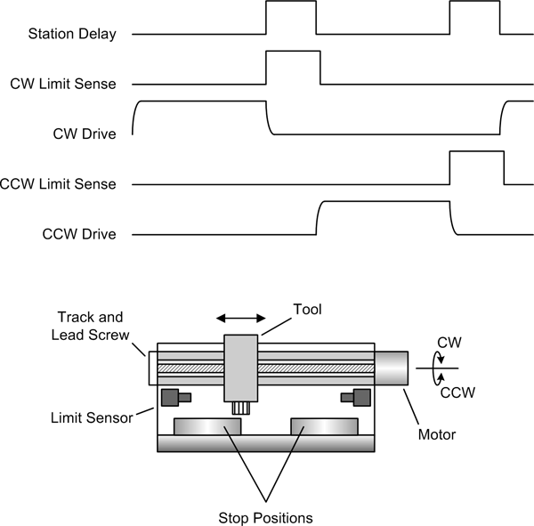
The mechanism has only one degree of freedom (one range of motion), either left or right, which in Figure 9-21 is shown as CW (clockwise) or CCW (counterclockwise) to indicate the rotation of the motor driving the lead screw. It doesn’t keep track of where the tool head is during travel; it only senses when the tool head is at one of the stop positions. The stop positions are determined by the physical positions of each of the end limit sensors.
In Figure 9-21, the motor activity indicated in the timing chart for CW Drive and CCW Drive has no sharp corners. This is because electric motors have inertia, and it takes some finite amount of time for the motor to come up to full speed, and some time for it to come to a complete stop when the power is removed. Notice that the state of the limit sensors changes as soon as the motor moves the tool off the limit in the opposite direction, but not when the motor starts, since it may take a little time to move off the limit sensor. Finally, we can assume that if the system is moving CW it doesn’t need to check the CCW limit sensor (which should be active), as it’s already there at the start of the movement. The same reasoning applies to CCW motion and the CW limit sensor.
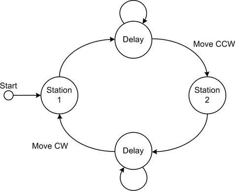
I mentioned earlier that a sequential control system can often be modeled as a state machine, and this is shown in the simplified state diagram in Figure 9-22. When the tool head reaches a limit sensor the motor (and motion) stops, and the system then waits (delays) for some period of time before sending the tool head back in the opposite direction. This cycle will repeat continuously until intentionally stopped.
In a real system, you would also want to incorporate some type of error checking: say, a timeout to determine if the motor has stalled and the tool head is stuck somewhere between the two limit sensors. If a fixed-speed motor is used, the time required for the tool head to move from one station to the other should be consistent to within a few tens of milliseconds, so you could also put in a time limit for moving the tool head between station positions. If the limit sensor takes too long to report a stop, there is probably something wrong that needs attention.
Sequential control systems are common in industrial process environments, and they are often implemented using programmable logic controller (PLC) devices. State diagrams are a common way to describe a sequential control system, and PLC technology has its own types of diagrams, known as ladder diagrams and sequential function charts (SFCs). Flowcharts can be used to model sequential systems, but they are actually too verbose for anything but the most trivial designs.
If you will be implementing sequential controllers, it would be worthwhile to explore what’s available in terms of diagram methodologies. Personally, I happen to prefer the SFC-type diagrams. They provide a slightly higher level of abstraction than a ladder diagram and are much more compact than a flowchart. Figure 9-23 shows an IEC 61131-3–type SFC.
In Figure 9-23, the heavy bars across the lines indicate a gating condition, which is some condition that needs to be true in order for the execution to proceed down a particular path. At each step there are actions that can be taken that will provide the inputs to a subsequent conditional test, or perform some system function.
An important thing to take away from Figure 9-23 is that a sequential controller doesn’t
just perform a series of steps in a fixed order; it can have branches to
alternate sequences as well. In other words, a sequential system can
incorporate if-then-type decision
points and conditional loops. A sequential control system can also
incorporate feedback in a closed-loop fashion.
Proportional, PI, and PID Controls
Proportional control is a key component in linear feedback control systems. A proportional controller is slightly more complex than a bang-bang controller, but it offers some significant advantages in terms of its ability to automatically accommodate a changing control environment and provide smooth, continuous linear control functionality. Purely proportional controls do have some drawbacks, though, including what is known as “droop,” and poor response behavior to sudden changes in the control input.
We’ve already seen some basic examples of proportional controls (e.g., in Figure 9-11), but now we’ll look at them in a bit more detail. We will then look at how the shortcomings of the purely proportional controllers can be dealt with by incorporating integral and derivative control modes into a system in the form of PI (proportional-integral) and PID (proportional-integral-derivative) controllers.
Off-the-shelf controllers versus software implementation
There are a number of commercial PID controllers available on the market for various applications. Some are intended specifically for temperature control, some are marketed as pressure controllers, and others are designed for motion control, to name a few applications. Prices vary, starting at around $100 for an entry-level PID servo controller, about $400 for an industrial-grade modular temperature controller, and upward of several thousand dollars for high-reliability industrial-grade units.
So, should you buy a PID controller, or should you write your own in software? The answer depends on how much you have in your budget for hardware components, what you have on hand in the way of data I/O devices, and how much time you are willing to spend implementing a custom PID algorithm and getting it running correctly.
If all you really need is a simple control system with acceptable impulse response, you might want to consider using something like the example Python code we’ll look at shortly. On the other hand, if your application needs a high degree of precision with fast real-time responses, you would most likely be better off purchasing a commercial controller. I should also point out that if you don’t really need a PI or PID controller for your application, you might as well save yourself the effort and not use one.
PID overview
In industrial control applications the most commonly encountered controller type is the PID, in both linear and nonlinear forms. Linear PID-type controls have been around in one form or another for over 100 years. In the earliest incarnations they were implemented as mechanical, hydraulic, or pneumatic devices based on levers, gears, valves, pistons, and bellows. As technology progressed, DC servos, vacuum tubes, and transistors were used. All of these designs operated in the continuous linear time domain. With the advent of computer-controlled systems the analysis and implementation of PID controls moved into the nonlinear and discrete-time domains, and topics such as sampling intervals and sample resolution became important design considerations. We’ll start here by looking at the basic theory behind PID controls in the continuous-time domain. Later we’ll see how a PID control can be implemented in software by translating it into the discrete-time domain.
A full PID controller is composed of three basic parts, or terms. These are shown in the block diagram in Figure 9-24.
The output of a PID control is just the sum of three terms:
Each has a specific role to play in determining the stability and response of the controller.
Mathematically, the control function for an ideal PID control can be written as shown in Equation 9-4.

where:
- e
Represents the system error (r – b)
- Kp
Represents the proportional gain
- Ki
Represents the integral gain
- Kd
Represents the derivative gain
- t
Represents instantaneous time
- u
Is the control output
- τ
Is the integral interval time (which may, or may not, be the same as t)
In practice, though, it’s more common to find the PID equation written like Equation 9-5.

Equations 9-4 and 9-5 both describe a PID control in the continuous-time domain. The primary difference between them is that in Equation 9-5 the gain parameter Kc is applied to all three terms, and the independent behavior of the I and D terms is determined by Ti and Td, which are defined as the integral time and the derivative time, respectively. I mention this because you may come across a PID description that uses a single gain variable, in what is called the standard form (Equation 9-6).

In a PID controller, the proportional term is the primary contributor to the control function, with the integral and derivative terms providing smaller (in some cases, much smaller) contributions. In fact, a PI controller is just a PID controller with the D term set to zero. You can also make a PID controller behave like a purely proportional control by setting the I and D terms to zero.
The proportional control term
A proportional control is a type of linear feedback control system, and we’ve already seen some examples of these types of systems (see Linear Control Systems). What I want to discuss here are some of the shortcomings of proportional controls as a prelude to the introduction of the I and D terms.
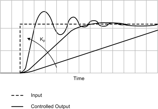
A proportional control works pretty well when the input changes slowly over time and there are no sudden jumps in the input level or in the feedback from the plant. However, proportional controls don’t handle sudden changes or transient events very well, and tend to exhibit overshoot, undershoot, and a reluctance to converge on the set-point (the reference input) if things are changing too rapidly. This is shown in Figure 9-25 for different values of Kp with a step input.
A step input is useful for control system response analysis, even if it will never be experienced by a control system in its operational setting. The main thing to take away from Figure 9-25 is how the gain variable Kp affects the ability of the control to respond to a quickly changing input and then damp out any swings around the set-point. A high gain setting will make for a more responsive system, but it will tend to overshoot and then dither around the set-point for a while. If the gain is set high enough it may never completely settle, and if the gain is set too high the entire system can go into oscillation. Conversely, if the gain is too low, the system will not be able to respond to input changes in a timely manner and it will have significant droop.
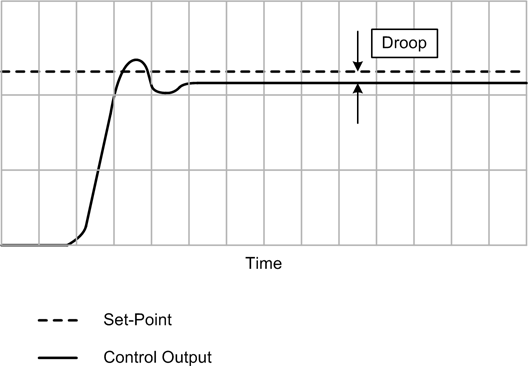
“Droop” is a problematic characteristic of proportional control systems wherein the output of the controller may never settle exactly at the set-point, but will instead exhibit a steady-state error in the form of a negative relative offset from the set-point. This is due largely to the difference between the gain of the controller and the gain of the process (or plant). Droop can be mitigated by applying a bias to the output of the controller, or it can be dealt with by using an integral term, as in a PI- or PID-type controller. Figure 9-26 shows the effect of droop.
There are also other external factors that affect how well a proportional control term will respond to control inputs. These include the responsiveness of the plant, time delays, and transient inputs.
PI and PID controls
The integral term, also known as the reset, is in effect an adaptive bias. The purpose of adding the integral term to the output of the controller is to account for the accumulated offset in the output and accelerate the output toward the set-point. Consequently, the proportional gain, Kp, must be lowered to account for the inclusion of the I term into the output.
If we recall that the error is the result of r – b, it should be apparent that the value of the integral term will increase rapidly when the error is largest, and then slow as the output converges on the reference input set-point and the error value goes to zero. So, the effect of the integral term will be to help to drive the system toward the set-point more rapidly than occurs with the P term alone. However, if Ki is too large, the system will overshoot, and it may become unstable. The effect of the integral term is dealt with when the controller is tuned for a particular application.
The derivative term in a full PID controller acts to slow the rate of change in the output of the controller. The effect is most pronounced as the control output approaches the set-point, so the net result of the derivative term is to limit or prevent overshoot. However, the derivative term also tends to amplify noise, and if Kd is too large, in the presence of transients and noise the control system may become unstable.
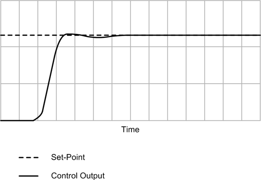
When all three terms are active and the controller is correctly tuned, it will exhibit a response like that shown in Figure 9-27.
Hybrid Control Systems
The distinction between sequential and linear control systems is not always clear-cut. It is not uncommon to find control systems that are a mix of various paradigms, because of the different subsystems that are incorporated into them.
Consider the control system one might find in a brewery for beer bottling. Such a system could be composed of various subsystems. One subsystem might control the bottle conveyor, and its function would be to ensure that empty bottles appear under a nozzle at specific times. In order to do this it must control the speed of the conveyor precisely, taking into account the weight of different bottle styles. Another subsystem might control the filling operation. It would need to sense when a bottle is under the nozzle and then dispense a specific amount of beer. The amount of beer to dispense could be a function of time (valve open for some number of seconds). You can extend this thought experiment further if you like, and it will soon become apparent that the beer-bottling part of a brewery is actually a rather complex system, itself consisting of many interrelated subsystems (some operating as sequential controls, others operating as linear controls, and perhaps even some nonlinear controls).
Implementing Control Systems in Python
We’ll start off by creating a simple linear closed-loop proportional control function. It may not look like much, but it has everything a basic proportional control requires. Next up is a nonlinear control in the form of a basic bang-bang controller. It has enough functionality to find immediate application as the controller for an air conditioning system, but it doesn’t handle heating. Adding the ability to control heating as well as cooling is straightforward, though, and shouldn’t present any significant challenge (it’s just the inverse of cooling).
Finally, we’ll look at a simple implementation of a basic linear PID controller, and find out how to translate the PID equation in Equation 9-4 into a discrete-time form that can be easily coded in Python.
In Chapter 10 I’ll present a simulator that can be used to obtain realistic data and generate response plots from the output of this function.
Linear Proportional Controller
A proportional controller is straightforward. Recall the basic equation we saw at the start of this chapter:
We can expand this a bit to explicitly incorporate the summing node with its r and b inputs, as shown in Equation 9-7.
Here is the code to implement Equation 9-7:
""" Simple proportional control.

    Obtains input data for the reference and the feedback, and
    generates a proportional control value using the equation:

    u = Kp(r – b) + P

    b is obtained from c * Kb, where c is the output of the
    controlled device or system (the plant), and Kb is a gain
    applied to scale it into the same range as the r (reference)
    input.

    The gain parameters Kp and Kb should be set to something
    meaningful for a specific application. The P parameter is
    the bias to be applied to the output.
"""
# local global variables. Set these using the module.varname
# external access method.
Kp = 1.0
Kb = 1.0
P  = 0

# replace these as appropriate to refer to real inputs
rinput = 0
cinput = 1

def PControl():
    rval = AnalogIn(rinput)
    bval = AnalogIn(cinput) * Kb
    eval = rval - bval
    return (Kp * eval) + P
In this example, the function AnalogIn() is just a dummy placeholder. You
will need to replace it, and the rinput and cinput variables, with something that makes
sense for your application.
Bang-Bang Controller
Recall from earlier that a bang-bang controller is a type of nonlinear control wherein the output is nonlinear, but it is a function of a linear input. In this example we’ll assume that the nonlinear output response is determined by two set-point values, one high and one low. When examining the following code, you might wish to refer to Equation 9-3 as a reference:
import time     # needed for sleep

# pseudo-constants
OFF = 0
ON  = 1

H = 2.0             # hysteresis range
delay_time = 0.1    # loop delay time

# replace these as appropriate to refer to real input and output
temp_sense = 0
device     = 0

def BangBang():
    do_loop = True
    sys_state = OFF

    while (do_loop):
        if not do_loop:
            break

        curr_temp = AnalogIn(temp_sense)     # dummy placeholder

        if curr_temp <= set_temp - H:
            sys_state = OFF

        if curr_temp >= set_temp + H:
            sys_state = ON

        # it is assumed that setting the port with the same value isn't
        # going to cause any problems, and the output will only change
        # when the port input changes
        SetPort(device, sys_state)           # dummy placeholder

        time.sleep(delay_time)
This function maps directly to Equation 9-3,
and it will behave as I described earlier, when we first looked at
nonlinear controls. As with the other examples in this section, it
doesn’t have error detection, and it could be extended to include the
ability to handle both heating and cooling. Also, the functions AnalogIn() and SetPort() are dummy placeholders, and the
variables temp_sense and device will need to be replaced with something
that matches the real execution environment.
Simple PID Controller
The first step in creating PID algorithms suitable for use with software is to convert from the continuous-time domain PID form in Equation 9-4 to a form in the discrete-time domain.
First, we formulate a discrete approximation of the integral term (Equation 9-8).

In this equation:
- e(i)
Is the error at integration step i
- i
Is the integration step
- Ts
Is the time step size (Δt)
Now for the derivative term (Equation 9-9).

In this equation:
- t
Is the instantaneous time
- e(t − 1)
Is the previous value of e, which is separated in time from e(t) by Ts
Just remember that we’re now in the discrete-time domain, and the t is there as a sort of placeholder to keep things temporally correlated.
We don’t really need to do anything with the proportional term from Equation 9-4; it’s already in a form that can be translated directly into code.
We can now substitute the discrete-time approximations in Equation 9-4 to obtain Equation 9-10.

In Equation 9-10:
- Ti
Is the integral time substep size
- Td
Is the derivative time substep size
- Ts
Is the time step size (Δt)
While this form does allow for fine-grained control in regard to time in order to generate better approximations of the integral and derivative term values, it often isn’t necessary to divide the overall Ts period into smaller slices for the integral and derivative terms. If we have a relatively fast control loop and we assume a unit time interval for all terms, Equation 9-10 can be simplified to Equation 9-11.

The following code listing shows a simple PID controller that implements the unit step time form from Equation 9-11:
class PID:
    """ Simple PID control.

        This class implements a simplistic PID control algorithm. When
        first instantiated all the gain variables are set to zero, so
        calling the method GenOut will just return zero.
    """
    def __init__(self):
        # initialize gains
        self.Kp = 0
        self.Kd = 0
        self.Ki = 0

        self.Initialize()

    def SetKp(self, invar):
        """ Set proportional gain. """
        self.Kp = invar

    def SetKi(self, invar):
        """ Set integral gain. """
        self.Ki = invar

    def SetKd(self, invar):
        """ Set derivative gain. """
        self.Kd = invar

    def SetPrevErr(self, preverr):
        """ Set previous error value. """
        self.prev_err = preverr

    def Initialize(self):
        # initialize delta t variables
        self.currtm = time.time()
        self.prevtm = self.currtm

        self.prev_err = 0

        # term result variables
        self.Cp = 0
        self.Ci = 0
        self.Cd = 0


    def GenOut(self, error):
        """ Performs a PID computation and returns a control value based
            on the elapsed time (dt) and the error signal from a summing
            junction (the error parameter).
        """
        self.currtm = time.time()               # get t
        dt = self.currtm - self.prevtm          # get delta t
        de = error - self.prev_err              # get delta error

        self.Cp = self.Kp * error               # proportional term
        self.Ci += error * dt                   # integral term

        self.Cd = 0
        if dt > 0:                              # no div by zero
            self.Cd = de/dt                     # derivative term

        self.prevtm = self.currtm               # save t for next pass
        self.prev_err = error                   # save t-1 error

        # sum the terms and return the result
        return self.Cp + (self.Ki * self.Ci) + (self.Kd * self.Cd)
Tuning a PID controller by adjusting the values of Kp, Ki, and Kd is often considered to be a black art. There are several approaches used for PID tuning, including the Ziegler-Nichols method, software-based automated tuning, and the trial-and-error method.
Here are some general rules of PID behavior that are useful for tuning a controller:
Kp controls the rise time. Increasing Kp results in a faster rise time, with more overshoot and longer settling time. Reducing Kp results in a slower rise time with less (or no) overshoot. The Kp term by itself is subject to droop.
Ki eliminates the steady-state error (droop). However, if Ki is set too high the control output may overshoot and the settling time will increase. Ki and Kp must be balanced to obtain an optimal rise time with minimal overshoot.
Kd provides a minor reduction in overshoot and settling time. Too much Kd can make the system unstable and cause it to go into oscillation, but a small value for Kd can improve the overall stability.
To use the PID control shown previously, you would first instantiate the controller and set the Kp, Ki, and Kd parameters:
pid = PID()
pid.SetKp(Kp)
pid.SetKi(Ki)
pid.SetKd(Kd)
A simple loop is used to read the feedback, call the PID method
GenOut(), and then send the control
value to the controlled device (the plant):
fb = 0
outv = 0

PID_loop = True

while PID_loop:
    # summing node
    err = sp - fb    # assume sp is set elsewhere

    outv = pid.GenOut(err)
    AnalogOut(outv)

    time.sleep(.05)

    fb = AnalogIn(fb_input)
Note that the set-point, sp,
must be set somewhere else before the loop is started. Alternatively,
you could call the PID control as part of a larger control loop, which
would then make it possible to change sp on the fly while the system is
running:
def GetPID():
    global fb

    err = sp - fb

    outv = pid.GenOut(err)
    AnalogOut(outv)

    time.sleep(.05)

    fb = AnalogIn(fb_input)
The system loop could also perform other functions, such as updating a user interface, processing acquired data, checking for errors, and so on:
while sys_active:
    # do some stuff
    UpdateUI()    # get sp from user
    GetPID()
    # do more stuff
If sp is a global variable in
the context of the system loop, the GUI might allow the user to change
it, and GetPID() will use it the next
time it is called.
Summary
This has been a very lightweight introduction to control systems theory and applications, and it is by no means complete. We have only skimmed the surface of the field of control systems theory and applications. This is a deep topic in engineering, drawing upon years of experience by an uncountable number of engineers and researchers.
It is my hope that you now have a general idea of what types of control systems can be built, how they work, and how to select the one that makes sense for your application.
Suggested Reading
If you would like to learn more about control systems and their applications, I would suggest that you pick up one (or more) of the following books:
- Advanced PID Control. Karl Åström and Tore Hägglund, ISA—The Instrumentation, Systems, and Automation Society, 2005.
If you want to dig deeper into control systems theory, and PID controls in particular, this book is a good place to start. It covers nearly every aspect of using PID controllers, and combines discussions of real-world examples with a solid presentation of the mathematical theory behind PID control technology. With chapters dealing with topics such as process models, controller design, and predictive control, it is a valuable resource for anyone working with control system technology.
- Introduction to Control System Technology, 7th ed. Robert Bateson, Prentice Hall, 2001.
I would recommend this book as a good starting point to learning about control systems and their applications. The math doesn’t require much more than first-year calculus, and the author employs numerous real-world examples to help illustrate the concepts. It also contains extensive definitions of terms in the form of chapter-specific glossaries and a section on basic electronics.
- Computer-Controlled Systems, 3rd ed. Karl Åström and Bjorn Wittenmark, Prentice Hall, 1996.
While it is well written (albeit a bit terse) and contains examples for Matlab® and Simulink®, this is probably not a book I would recommend as a first read on the subject of control systems. It is, however, a good reference once you’ve gotten your feet wet and need to find insight into specific problems. If you work with control systems on a regular basis (or you’re planning on it), I’d recommend this book as a handy reference and for advanced study.
- Real Time Programming: Neglected Topics, 4th ed. Caxton C. Foster, Addison-Wesley, 1982.
Foster’s book is a short, concise treatment of various topics relevant to real-time data acquisition and control systems. Well written with a light and breezy style, the book contains several short chapters dealing with basic control systems theory using a minimal amount of mathematics. It also covers the basics of digital filters, signal processing, and constrained communications techniques, among other topics. It has been out of print for a long time, but it is still possible to find used copies.
There are also numerous websites with excellent information on control systems, and even some software available for free. Here are a few to start off with:
- http://citeseerx.ist.psu.edu/viewdoc/download?doi=10.1.1.129.1850&rep=rep1&type=pdf
PDF version of the book Feedback Control Theory, by John Doyle, Bruce Francis, and Allen Tannenbaum (Macmillan, 1990). It can also be purchased in paperback form. Oriented toward classical control theory and transfer function analysis, this book is a good introduction to advanced concepts. Its particular emphasis is on robust performance.
- http://aer.ual.es/modelling/
Home site for a set of excellent interactive learning modules from the University of Almeria (Spain). Check this out after you’ve spent some time reading through one of the books cited previously; the interactive applets are very useful for dynamically illustrating various control system concepts. The module on PID controls is a companion resource for the book Advanced PID Control. Note that the commercial site for the Swiss company Calerga Sarl at http://www.calerga.com/contrib/index.html hosts the same learning modules.
- http://www.cds.caltech.edu/~murray/amwiki/index.php/Main_Page
Karl Åström’s and Richard Murray’s wiki. Contains the complete text of the book Feedback Systems: An Introduction for Scientists and Engineers (Princeton University Press), along with examples and additional exercises. This is a good introduction to feedback control systems that doesn’t shy away from the necessary mathematics. But even if your memories of calculus are a bit fuzzy, you should still find plenty to take away from this book.
- http://www.me.cmu.edu/ctms/controls/ctms/pid/pid.htm
A collection of control system tutorials written for use with Matlab and Simulink.
And, of course, Wikipedia has numerous articles on control systems topics.