APPENDIX B
Constructing the Value Curve
THE VALUE CURVE is deeply rooted in the very different way that Toyota looks at measuring its business. Taiichi Ohno, the architect of the Toyota Production System, disagreed with the way that traditional companies set the prices for their products.
When we apply the cost principle selling price = profit + actual cost, we make the customer responsible for every cost. This principle has no place in today’s competitive automobile industry.… The question is whether or not the product is of value to the buyer.1
Toyota shifts the equation around in a way that is mathematically equivalent but creates an entirely different meaning: selling price – actual cost = profit. The company recognizes that customers—not the company—assess the value of its products. And, like it or not, it is customer perception of value that forms the basis for pricing. Setting a sticker price higher than this will only drive customers to competitors’ more reasonably priced products.
Profits, therefore, are not set by the company; they are simply the difference between what the customer is willing to pay (their perceived value) and what it takes the company to produce it. Toyota’s approach is two pronged: increase the perceived value of the product and decrease the cost of turning it out.
But another key factor affects this result: the changing circumstances that impact both how the customer perceives the product’s value and the company’s ability to create it. In a downward economy, customers look at value differently; not only do they have less to spend, but they more closely scrutinize the benefit they get from their purchases. These same pressures might impact the corporations by driving them to produce at a rate below the point at which they operate efficiently.
This impact of uncertainty and changes on both components of value is depicted by the value curve. The shape of the curve offers powerful insights into the relationship between customers’ perception of what the organization offers and its ability to turn it out across the range of conditions that mark today’s business environment. A steep, U-shaped value curve points to an underlying structure that thrives amid stability but does not respond well when it is forced to shift too far from its intended condition. A company that has reached an advanced state of lean dynamics maturity exhibits a flat curve, demonstrating its ability to sustain value across a range of conditions.
The Elements of the Value Curve
The value curve is simply a graphic representation of the company’s ability to generate bottom-line, tangible value as it responds to the broad range of dynamic conditions it must face. It is constructed by presenting the proportional relationship (not the raw data) between a business’s two elements of value—value available and value required—on a graph to show how it changes across the range of conditions they face. The following is a description of the chart’s major elements:
![]() Value available is the tangible measure of customer value—how much a company gains through sales of its products and services to its customers. It is termed value available because this becomes the value that the company has available for all that it does. This is based on the company’s net sales, a measure of what the customer pays for what it turns out.
Value available is the tangible measure of customer value—how much a company gains through sales of its products and services to its customers. It is termed value available because this becomes the value that the company has available for all that it does. This is based on the company’s net sales, a measure of what the customer pays for what it turns out.
![]() Value required is the total cost of creating this value for the customer. It represents the portion of the value available that applies to all of the activities, expenditures, and even wastes in turning out products and services and selling them to the customer. It is based on the net sales minus the net income during a given timeframe (usually a fiscal year). It should only include costs related to normal business activities; it should exclude unrelated gains or expenditures, like those from large investments or revenues from selling major business units.
Value required is the total cost of creating this value for the customer. It represents the portion of the value available that applies to all of the activities, expenditures, and even wastes in turning out products and services and selling them to the customer. It is based on the net sales minus the net income during a given timeframe (usually a fiscal year). It should only include costs related to normal business activities; it should exclude unrelated gains or expenditures, like those from large investments or revenues from selling major business units.
![]() The horizontal axis represents a measure of the range of operating conditions across which these measures of value will be displayed. This usually measures sales volume and is selected based on the way value is delivered to the customer. For the automotive industry, unit sales volume can be used. For retail, this is depicted as sales per store; the measure for the airline industry is volume of passengers transported per flight (known as “load factor”).
The horizontal axis represents a measure of the range of operating conditions across which these measures of value will be displayed. This usually measures sales volume and is selected based on the way value is delivered to the customer. For the automotive industry, unit sales volume can be used. For retail, this is depicted as sales per store; the measure for the airline industry is volume of passengers transported per flight (known as “load factor”).
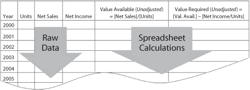
The value curve is intended to display the relationship between value available and value required across the company’s range of operating conditions—not the absolute measures, which means that adjustments to these raw data must be made to make their proportional relationships clear.
Figure B-1. Raw Data for Value Curve Construction
Performing Value Curve Calculations
The first step is to capture the basic information from a range of sequential years when the company’s approach remains fairly consistent. It might have grown in size, for instance, but it is important that no major shift in approach (such as a corporate merger or a major shift in technology) occurred during the time-frame represented.
Capturing the basic data and performing value curve calculations is easiest on a spreadsheet. Begin by creating rows for each of the years that will be included in the assessment. Because assessing an organization’s performance means pressing it to its limits, it is important to include data from successive years during which it is subjected to as much of the full range of conditions that might occur throughout its operation. Figure B-1 is a notional depiction of how a spreadsheet might be populated using data representing a company’s performance during a sequence of years.
The value curve is intended to display the proportional relationship between value available and value required; therefore, it is depicted in a way that makes these proportional relationships clear—something that would be hard to visualize if we simply plotted raw data. The pattern that would result would be like that depicted in Figure B-2.
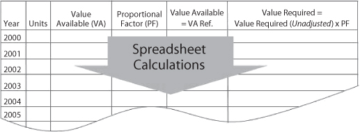
Instead, we can accomplish this by displaying them as a ratio, holding value required as a constant and displaying value available as a calculated proportion. For instance, the value available might be set as the maximum level for the range of years listed, identified as VA Ref. in Figure B-3; the proportional factor for each value added would then become PF = (VA Ref.)/VA. Each VA in Figure B-3 would have a different proportional factor (PF), which would be multiplied by the value required (VR) representing that year to result in the proportional value required (the final column in the spreadsheet notionally depicted by Figure B-3).
As shown here, the calculations involved in constructing a value curve are fairly straightforward. They involve simple arithmetic that can readily be calculated on a standard spreadsheet. However, much thought must be given to what the results represent. For instance, creating a value curve for a manufacturer that produces different variants of the same basic product or service is fairly simple (as in the case of an automotive producer in our example). It becomes much more difficult to determine how to portray value for a conglomerate that produces widely ranging products and services. In these cases, it might be better to break out parts of the business that turn out more consistent types of value, and map these separately. For simplicity, value required and value available can be calculated for a corporation as a whole (using net sales and net income) rather than applying the calculations by unit.
Figure B-2. Value Available Versus Value Required2
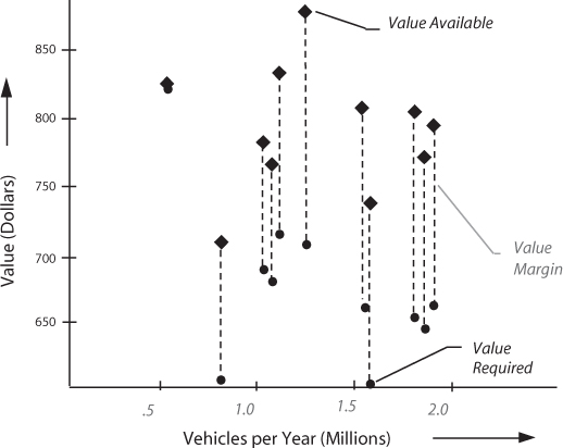
Figure B-3. Spreadsheet Calculations for Plotting Value Curve
Another important element is the identification of the units of measure for the horizontal axis. For this example, the annual sales of vehicles serves as an excellent representation of the impact that changing conditions have on the business and represents how vehicles are sold to the customer (as individual units). As indicated earlier in this appendix, a powerful measure used for an airline’s value curve is the passenger load factor. This data is widely available (it is a standard industry measure), and it represents how business conditions affect its unit of value delivery to the customer: how many people purchase a passenger flight. A measure used for a supermarket might be total sales per store, since this represents the impact of changing conditions at the point at which customers purchase what it offers.
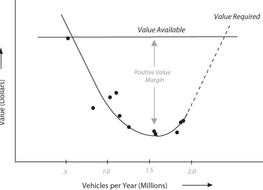
Now the data can be plotted on a graph, as shown in Figure B-4 (note that the fifth column, which is constant, and sixth column are each plotted on the vertical axis, against the volume for that year, or the second column, on the horizontal axis). The example depicted in the figure is the same as that displayed in Figure 2-1 (early GM’s performance from market peak to the Great Depression, whose calculations were originally depicted in Going Lean).
It is important to note that this approach depends on the ability to measure a stable system over time, and applies only for those time frames in which no major shift in approach is introduced. It then stands to reason that the shape of the curve-often the classic U-shape depicted in Figure B-4—is driven purely by the way that the company or institution responds to its environment. What comes next is to understand the causes for this—the sources of lag that cause the business or institution to respond so poorly when conditions extend beyond those for which it was designed.
Figure B-4. The Value Curve 3
Interpreting the Value Curve
A key step is for businesses and institutions to build a comprehensive understanding of how these real and potential external forces stand to impact their business. This is a critical but often neglected foundation for lean transformation.
Potential Value Curve Indications
The value curve offers the ability to create a baseline understanding of the organization’s capability to turn out stable value across a range of conditions. A steep value curve serves as an initial indication that a problem exists. However, the value curve is only a starting point; its real utility is in driving probing questions that support the dynamic value assessment outlined in Appendix A. Some areas of questions include the following:
![]() How responsive to changing conditions are the business’s or institution’s operations? How well do the company’s performance metrics correlate efficiency gains for internal processes to bottom-line results? Do they track responsiveness to dynamic conditions? Are the mechanisms for scheduling operations generally rigid and driven from the top down, causing workarounds when change suddenly strikes? How badly do shifts in customer demand or disruptions to the business environment drive shifts in how business is done?
How responsive to changing conditions are the business’s or institution’s operations? How well do the company’s performance metrics correlate efficiency gains for internal processes to bottom-line results? Do they track responsiveness to dynamic conditions? Are the mechanisms for scheduling operations generally rigid and driven from the top down, causing workarounds when change suddenly strikes? How badly do shifts in customer demand or disruptions to the business environment drive shifts in how business is done?
![]() Does the business’s or institution’s organizational construct respond well to change? Is it marked by a steep management hierarchy, leading to long decision cycles? Do decision-making roles shift during times of crisis? Are supplier arrangements strictly managed by outcome-based targets, or do they focus on creating dynamically stable capabilities? Do people within the organization have the span of insight to step in to help get things done when needed?
Does the business’s or institution’s organizational construct respond well to change? Is it marked by a steep management hierarchy, leading to long decision cycles? Do decision-making roles shift during times of crisis? Are supplier arrangements strictly managed by outcome-based targets, or do they focus on creating dynamically stable capabilities? Do people within the organization have the span of insight to step in to help get things done when needed?
![]() Is information compartmentalized and complex? Can people at different parts and levels within the organization clearly see how their activities and decisions support bottom-line outcomes? Are data broken down to support simple and meaningful metrics? Do these clearly relate to the creation of customer and corporate value (rather than lagging factors like inventory) at each station along the way?
Is information compartmentalized and complex? Can people at different parts and levels within the organization clearly see how their activities and decisions support bottom-line outcomes? Are data broken down to support simple and meaningful metrics? Do these clearly relate to the creation of customer and corporate value (rather than lagging factors like inventory) at each station along the way?
![]() Is creating innovation a central part of doing business? What mechanisms are in place to promote product and process innovations from all areas of the organization (including the supplier base) and to streamline their introduction into operations? How does the company or institution seek to advance the types of opportunities it pursues (described in Chapter 9), and how does this drive its advancement toward maturity?
Is creating innovation a central part of doing business? What mechanisms are in place to promote product and process innovations from all areas of the organization (including the supplier base) and to streamline their introduction into operations? How does the company or institution seek to advance the types of opportunities it pursues (described in Chapter 9), and how does this drive its advancement toward maturity?
![]() How well are lean capabilities integrated into the business strategy? Are advancements in lean dynamics capabilities and maturity viewed by top executives as a central driver for expanding customer and corporate value? Is leveraging these improvements fundamental to the organization’s vision and strategy?
How well are lean capabilities integrated into the business strategy? Are advancements in lean dynamics capabilities and maturity viewed by top executives as a central driver for expanding customer and corporate value? Is leveraging these improvements fundamental to the organization’s vision and strategy?
The Value Curve as a Basis for Performance Measurement
It is important to recognize that the purpose of plotting the value curve is simply to show how the relationship between value available and value required varies across a range of circumstances—what is important is not so much the curve, but the value margin. Recognizing that attaining a strong, consistent value margin is really what lean dynamics is all about sets the stage for identifying metrics that meet the criteria identified in Chapter 6—in essence, to promote an expanded span of insight at all levels, and drive action that is consistent with the organization’s short-term and long-term lean vision.
Relating value margins to individual activities and operating elements can therefore create a valuable linkage to desired bottom-line results. It offers potential to serve as an effective means for relating all that is going on across the business—from planning to actual performance, showing the real operational capability to respond to change. The result might be seen as analogous to Southwest Airlines’ approach to keeping everyone across the business aware of the bottom-line impact of his or her work to creating value (described in Going Lean). This can serve as a tremendous enabler to driving down organizational lag, and creating a consistent, business-wide mindset toward attaining a level of sustainable lean.