CHAPTER 4
PAIRED MEASUREMENTS DATA
4.1 PREVIEW
Even though the paired measurements design is not a good choice for method comparison studies, it remains by far the most commonly used design in practice. This chapter coalesces ideas from previous chapters to present a methodology for analysis of paired measurements data. The methodology follows the steps outlined in Section 1.16. Modeling of data via either a mixed-effects model or a bivariate normal model is considered. Evaluation of similarity and agreement under the assumed model is taken up next. Three case studies are used to illustrate the methodology.
4.2 MODELING OF DATA
4.2.1 Mixed-Effects Model
The data consist of paired measurements (Yi1, Yi2), i = 1,...,n, by two measurement methods on n randomly selected subjects from a population. In principle, there are two choices for modeling these data (Section 1.12). The preferred one is the mixed-effects model (1.19), which is written as
 (4.1)
(4.1)where
- the true values bi follow independent N1(µb,
 ) distributions,
 - the random errors eij follow independent
 distributions, j = 1, 2, and
 - the true values and the random errors are mutually independent.
This model implicitly assumes that the methods have the same scale (Section 1.12.2). The paired measurements are i.i.d. as (Y1, Y2), and their differences Di = Yi2 − Yi1 are i.i.d. as D. From (1.20), (1.21), and (1.24), we have
 (4.2)
(4.2)The ML estimates—![]() —of model parameters can be obtained by using a statistical software for fitting mixed-effects models. In fact,
—of model parameters can be obtained by using a statistical software for fitting mixed-effects models. In fact,
 (4.3)
(4.3)and often the other estimates can be obtained explicitly as well (Exercise 4.2). It is a good idea to examine especially the estimates of error variances and their standard errors to ensure that they are estimated reliably (Section 1.12.2). The predicted random effects ![]() are
are
 (4.4)
(4.4)and the fitted values ![]() and the residuals
and the residuals ![]() are (Exercise 4.3)
are (Exercise 4.3)
 (4.5)
(4.5)The model adequacy is checked by performing model diagnostics (Section 3.2.4). Mild departures from normality of either residuals or random effects are not of much concern because generally they do not lead to seriously incorrect estimates of parameters of interest and their standard errors. However, presence of a trend or nonconstant scatter in the residual plot casts doubt on the respective assumptions of independence of true values and errors and homoscedasticity of error distributions. Moreover, a trend in the Bland-Altman plot (Section 1.13) may indicate violation of the equal scales assumption. These violations may not be benign because, in this case, the extent of agreement between the methods depends on the magnitude of measurement, contradicting what is implied by the model. Often, these assumptions hold after a log transformation of the data. These plots may also reveal outliers. If they are present and cannot be attributed to coding errors, their influence should be examined as well. At the minimum, this involves analyzing data with and without the outliers and comparing the key conclusions. During model evaluation we are not interested in checking whether a submodel with ![]() provides an equally good but a more parsimonious fit to the data. We let each of the two methods have its own accuracy and precision-related parameters under our model, and use inference on measures of similarity (Section 1.7) to examine their closeness. The differences in these marginal characteristics of the methods are also reflected in the measures of agreement.
provides an equally good but a more parsimonious fit to the data. We let each of the two methods have its own accuracy and precision-related parameters under our model, and use inference on measures of similarity (Section 1.7) to examine their closeness. The differences in these marginal characteristics of the methods are also reflected in the measures of agreement.
4.2.2 Bivariate Normal Model
Quite often, the error variances in the mixed-effects model (4.1) are not estimated reliably (Section 1.12.2). This is evident when at least one of the estimates has a rather large standard error, or when one of the estimates is nearly zero and the other is substantially larger. Generally this happens because the paired measurements do not have enough information to reliably estimate the error variances. In this case, we fit the bivariate normal model (Section 1.12.3), which simply postulates that the paired measurements are i.i.d. as (Y1, Y2), where
 (4.6)
(4.6)with σ12 = ρσ1 σ2 and ρ denoting the correlation. It follows that the differences Di are i.i.d. as D, where
 (4.7)
(4.7)Unlike (4.1), this model does not make any assumptions about the relationship between the observed measurements, their underlying true values, and the random errors. Neither does it require the assumption of a common scale for the methods. Further, the methods have a positive correlation under (4.1), whereas there is no such constraint here. However, the methods in practice do tend to have a positive correlation.
The use of a bivariate normal model has consequences for evaluation of similarity of methods (Section 1.12.3), but reliable estimation of its parameters is generally not an issue. The ML estimators of these parameters and of their functions appearing in (4.7) are given by their sample counterparts (Exercise 4.1),
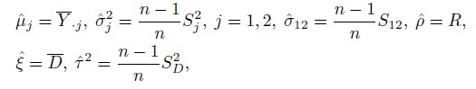 (4.8)
(4.8)where the sample moments are from (1.16) and (1.17).
Checking the adequacy of the fitted bivariate normal model involves examining the assumptions of normality and homoscedasticity of data. Bivariate normality can be assessed by using normal Q-Q plots to examine marginal normality of paired measurements as well as their linear combinations such as means and differences. The marginal Q-Q plots can be supplemented by a χ2 Q-Q plot for direct assessment of bivariate normality (Section 3.2.4). The homoscedasticity assumption can be verified by examining the Bland-Altman plot (Section 1.13.3) and a trellis plot of the data. Absence of a trend in the Bland-Altman plot is suggestive of common scales for the methods. In this case, the mean difference µ2 − µ1 can be interpreted as the fixed bias difference β0 (Section 1.7). These plots may also reveal outliers. As usual, if outliers are present, their influence needs to be investigated by analyzing data with and without them and comparing the conclusions of interest.
Here we have presented the bivariate normal model (4.6) as a fallback to the mixed-effects model (4.1) for the situation when the estimation of error variances is problematic. However, if ρ > 0, one may think of (4.6) as (4.1) with model parameters reparameterized as first-and second-order population moments of (Y1, Y2),
 (4.9)
(4.9)Under certain conditions (given in Exercise 4.2), the ML estimators of these moments are identical under the two models.
4.3 EVALUATION OF SIMILARITY AND AGREEMENT
Under the mixed-effects model, the methods have the same scale and hence their sensitivity ratio is identical to the precision ratio (Section 1.7). Therefore, the methods differ only in two marginal characteristics—fixed biases and precisions. Thus, similarity can be evaluated by examining estimates and two-sided confidence intervals for the intercept β0 and the precision ratio ![]() . If λ is not estimated reliably, possibly because the estimated error variances have large standard errors, the confidence interval of λ will be unreliable. In this case, we have to forgo comparing precisions of the methods. This point is moot if we switch to the bivariate normal model.
. If λ is not estimated reliably, possibly because the estimated error variances have large standard errors, the confidence interval of λ will be unreliable. In this case, we have to forgo comparing precisions of the methods. This point is moot if we switch to the bivariate normal model.
The bivariate normal model does not allow inference on any measure of similarity (Section 1.12.3). Nevertheless, one can compare the means and variances of the methods by examining estimates and two-sided confidence intervals for the mean difference µ2 − µ1 and the variance ratio ![]() . Of course, µ2 − µ1 equals β0 under the equal scales assumption, but in general the two may differ because the differences in fixed biases and scales of the methods get confounded in µ2 − µ1, see (1.10). Even then, if the mean difference is close to zero we can often conclude that the methods have similar fixed biases and scales. The inference on variance ratio, however, may not be that informative. From (1.8), the differences in scales and error variances get confounded in
. Of course, µ2 − µ1 equals β0 under the equal scales assumption, but in general the two may differ because the differences in fixed biases and scales of the methods get confounded in µ2 − µ1, see (1.10). Even then, if the mean difference is close to zero we can often conclude that the methods have similar fixed biases and scales. The inference on variance ratio, however, may not be that informative. From (1.8), the differences in scales and error variances get confounded in ![]() . Since the between-subject variation typically dominates the within-subject variation, the variance ratio may be close to 1 regardless of whether or not the precision ratio is close to 1.
. Since the between-subject variation typically dominates the within-subject variation, the variance ratio may be close to 1 regardless of whether or not the precision ratio is close to 1.
To evaluate agreement between the methods, we can take any scalar agreement measure that is a function of parameters of the bivariate distribution of (Y1, Y2), replace the population quantities in its definition by their counterparts under the assumed model, and examine its estimate and appropriate one-sided confidence bound. For example, recall the CCC and TDI defined by (2.6) and (2.29), respectively. They are
 (4.10)
These measures can be used directly under the bivariate normal model. Under the mixed-effects model, these can be expressed by replacing the population moments of (Y1, Y2) and D by their model-based counterparts in (4.2) to obtain
 (4.11)
For both the mixed-effects and bivariate models, the ML estimators of measures of similarity and agreement are obtained by replacing the model parameters in their definitions with their ML estimators. Then, the large-sample theory of ML estimators is used to compute standard errors and confidence bounds and intervals (Section 3.3). Further, the 95% limits of agreement are given as
 (4.12)
where ![]() and
and ![]() are given in (4.8).
are given in (4.8).
For the mixed-effects model, if the difference β0 in fixed biases is appreciable, it may be reasonable to reevaluate agreement by transforming method 2 measurements as ![]() . For this, one can simply repeat the analysis by subtracting β0 from method 2 measurements. We can achieve a similar end for the bivariate normal model by using the mean difference µ2 − µ1 in place of β0, provided the equal scales assumption holds.
. For this, one can simply repeat the analysis by subtracting β0 from method 2 measurements. We can achieve a similar end for the bivariate normal model by using the mean difference µ2 − µ1 in place of β0, provided the equal scales assumption holds.
4.4 CASE STUDIES
We now revisit the three datasets introduced in Section 1.13 and analyze them using the methodology described in this chapter. The analysis follows the five key steps outlined in Section 1.16, namely, visualization, modeling, evaluation of similarity, evaluation of agreement, and review of causes of disagreement. The last step is aimed at a recalibration strategy to increase agreement between the methods. Here and elsewhere in the book the unit of measurement is generally mentioned with the data description and is omitted thereafter for brevity.
4.4.1 Oxygen Saturation Data
This dataset, introduced in Section 1.13.1, consists of measurements of percent saturation of hemoglobin with oxygen in 72 adults, obtained using an oxygen saturation monitor (OSM, method 1) and a pulse oximetry screener (POS, method 2). The scatterplot and the Bland-Altman plot of these data shown in Figure 1.3 indicate that the methods are highly correlated and have similar scales. The trellis plot of these data displayed in Figure 4.1 shows some overlap in the readings produced by the methods, but it is also apparent that POS measurements tend to be smaller than OSM, especially in the middle of the measurement range. The data appear homoscedastic.
We first fit the mixed-effects model (4.1). But ![]() has a large standard error (Exercise 4.4), leading us to question the reliability of the estimate. Therefore, we prefer the bivariate normal model (4.6). The resulting ML estimates and standard errors are presented in Table 4.1. None of the estimates has an unusually large standard error. The adequacy of bivariate normality is checked in Exercise 4.4. Substituting these estimates in (4.6) gives the fitted distributions of (Y1, Y2) and D as follows:
has a large standard error (Exercise 4.4), leading us to question the reliability of the estimate. Therefore, we prefer the bivariate normal model (4.6). The resulting ML estimates and standard errors are presented in Table 4.1. None of the estimates has an unusually large standard error. The adequacy of bivariate normality is checked in Exercise 4.4. Substituting these estimates in (4.6) gives the fitted distributions of (Y1, Y2) and D as follows:

Clearly, POS measurements are on average a bit smaller than OSM, and both methods have similar variabilities. The correlation between the methods is 0.99. The differences in measurements have a standard deviation of 1.2. Further, the 95% limits of agreement from (4.12) are (−2.77 , 1.94).
For similarity evaluation under the bivariate normal model, we must be content with inference on the mean difference µ2 − µ1 and the variance ratio ![]() . The estimate of µ2 − µ1 is − 0.41 and its 95% confidence interval is (−0.69, − 0.13). Thus, there is evidence that the mean for POS is slightly smaller than OSM. But this difference may be considered negligibly small because the measurements range between 70 and 100, with the average around 89. Note that this µ2 − µ1 can be interpreted as β0 as the equal scales assumption appears reasonable for these data. The estimate of
. The estimate of µ2 − µ1 is − 0.41 and its 95% confidence interval is (−0.69, − 0.13). Thus, there is evidence that the mean for POS is slightly smaller than OSM. But this difference may be considered negligibly small because the measurements range between 70 and 100, with the average around 89. Note that this µ2 − µ1 can be interpreted as β0 as the equal scales assumption appears reasonable for these data. The estimate of ![]() is 1.02 and its 95% confidence interval is (0.95, 1.08), confirming similar variances for the methods.
is 1.02 and its 95% confidence interval is (0.95, 1.08), confirming similar variances for the methods.
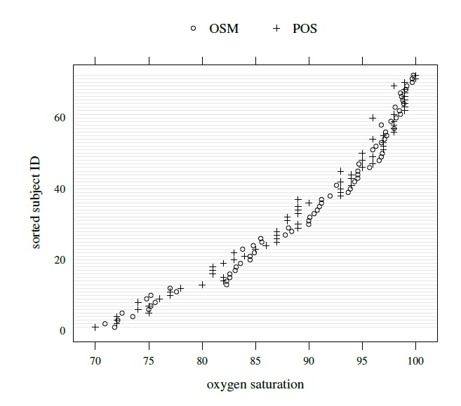
Figure 4.1 Trellis plot of oxygen saturation data.
The next step is evaluation of agreement. Table 4.1 also provides estimates and 95% one-sided confidence bounds for agreement measures CCC and TDI(0.90). A lower bound is provided for CCC, whereas an upper bound is provided for TDI. For greater accuracy in estimation, the confidence bounds are computed by first applying the Fisher’s z-transformation to CCC and the log transformation to TDI, and then transforming the results back to the original scale (Section 3.3.3). The estimate 0.989 and the lower bound 0.984 for CCC indicate a high degree of agreement between the methods. Nonetheless, a high CCC is almost guaranteed here because the between-subject variation in the data is much greater than the within-subject variation (see Figure 4.1). More informative are the estimate 2.09 and upper bound 2.40 for TDI(0.90). From the tolerance interval interpretation of TDI’s upper bound (Section 2.8), it follows that 90% of differences in OSM and POS measurements lie within ±2.40 with 95% confidence. Given that the measurements range between 70 and 100, a difference of 2.4 may be considered too small to be clinically important.
As the methods differ in means (or fixed biases under the equal scales assumption), it is of interest to recalibrate POS by subtracting ![]() from its measurements, and reevaluate its agreement with OSM. Of course, the estimated means are identical after recalibration, but there is only a slight improvement in the extent of agreement. The estimate of CCC and its lower bound, respectively, increase to 0.990 and 0.986, and the estimate of TDI(0.90) and its upper bound, respectively, decrease to 1.98 and 2.27. The conclusion here is that if a difference in OSM and POS of 2.4 is considered clinically unimportant, then these methods agree sufficiently well to be used interchangeably. This conclusion holds regardless of whether POS is recalibrated or not.
from its measurements, and reevaluate its agreement with OSM. Of course, the estimated means are identical after recalibration, but there is only a slight improvement in the extent of agreement. The estimate of CCC and its lower bound, respectively, increase to 0.990 and 0.986, and the estimate of TDI(0.90) and its upper bound, respectively, decrease to 1.98 and 2.27. The conclusion here is that if a difference in OSM and POS of 2.4 is considered clinically unimportant, then these methods agree sufficiently well to be used interchangeably. This conclusion holds regardless of whether POS is recalibrated or not.
Table 4.1 Summary of estimates of bivariate normal model parameters and measures of similarity and agreement for oxygen saturation data. Lower bound for CCC and upper bound for TDI are presented. Methods 1 and 2 refer to OSM and pulse, respectively.
| Parameter | Estimate | SE |
| μ1 | 89.50 | 1.02 |
| μ2 | 89.08 | 1.03 |
| 4.31 | 0.17 | |
| 4.33 | 0.17 | |
| z(ρ) | 2.67 | 0.12 |
| z(CCC) | 2.61 | 0.12 |
| log{TDI(0.90)} | 0.74 | 0.08 |
| Similarity Evaluation | ||
| Measure | Estimate | 95% Interval |
| μ2 ‒ μ1 | ‒0.41 | (‒0.69, ‒0.13) |
| 1.02 | (0.95, 1.08) | |
| Agreement Evaluation | ||
| Measure | Estimate | 95% Bound |
| CCC | 0.989 | 0.984 |
| TDI(0.90) | 2.091 | 2.397 |
4.4.2 Plasma Volume Data
This dataset, introduced in Section 1.13.2, consists of measurements of plasma volume in 99 subjects using the Hurley method (method 1) and the Nadler method (method 2). Unlike the oxygen saturation data, these data show a difference in proportional biases of the methods. But it vanishes after a log transformation and the assumption of equal scales is satisfied for log-scale measurements. The trellis plot in Figure 1.10 shows that, with only a few exceptions, the Nadler measurements are higher than Hurley’s by nearly a constant amount. Of course, this indicates unequal fixed biases of the methods. The data seem homoscedastic.
First we fit the mixed-effects model (4.1) and Table 4.2 summarizes the results. None of the standard errors is especially large, and ![]() has a small standard error. This is not surprising given the near constancy of differences seen in the trellis plot. Figure 4.2 presents the residual plot from the fitted model. Lack of any discernible pattern in this plot supports the model. Evaluation of normality assumption is taken up in Exercise 4.5. For comparison, Table 4.2 also presents estimates resulting from fitting the bivariate normal model to the
has a small standard error. This is not surprising given the near constancy of differences seen in the trellis plot. Figure 4.2 presents the residual plot from the fitted model. Lack of any discernible pattern in this plot supports the model. Evaluation of normality assumption is taken up in Exercise 4.5. For comparison, Table 4.2 also presents estimates resulting from fitting the bivariate normal model to the
Table 4.2 Summary of estimates of model parameters and measures of similarity and agreement for log-scale plasma volume data. Lower bound for CCC and upper bound for TDI are presented. Methods 1 and 2 refer to Hurley and Nadler methods, respectively.
| Mixed-Effects Model | Bivariate Normal Model | ||||
| Parameter | Estimate | SE | Parameter | Estimate | SE |
| β0 | 0.10 | 0.002 | µ1 | 4.48 | 0.02 |
| µb | 4.48 | 0.02 | µ2 | 4.58 | 0.02 |
| −3.69 | 0.14 | −3.67 | 0.14 | ||
| −8.07 | 1.11 | −3.68 | 0.14 | ||
| −8.78 | 2.25 | z(ρ) | 2.69 | 0.10 | |
| Both Models | ||
| Parameter | Estimate | SE |
| z(CCC) | 1.19 | 0.07 |
| log {TDI(0.90)} | −2.07 | 0.02 |
| Similarity Evaluation | ||
| Measure | Estimate | 95% Interval |
| β0 (or µ2 − µ1) | 0.099 | (0.095, 0.103) |
| 0.994 | (0.942, 1.048) | |
| Agreement Evaluation | ||
| Measure | Estimate | 95% Bound |
| CCC | 0.830 | 0.792 |
| TDI(0.90) | 0.127 | 0.132 |

Figure 4.2 Residual plot for logscale plasma volume data.
data. As expected, both models lead to the same fitted distributions of (Y1, Y2) and D;

We see that log-scale measurements of Nadler exceed those of Hurley by 0.10 on average, the measurements have similar variabilities, and their correlation is 0.99. From (1.4), both methods have reliabilities around 0.99. The differences have a small standard deviation. The 95% limits of agreement are (−0.04, 0.23).
To evaluate similarity, Table 4.2 provides an estimate of 0.10 and a 95% confidence interval of (0.095, 0.103) for β0. The interval is tight around 0.10, confirming unequal fixed biases of the methods. As in the previous case study, we have to forgo inference on the precision ratio λ because its estimate has a large standard error (Exercise 4.5). Nevertheless, the estimated variance ratio ![]() is practically 1 with 95% confidence interval (0.94, 1.05).
is practically 1 with 95% confidence interval (0.94, 1.05).
To evaluate agreement, Table 4.2 provides estimates and 95% one-sided confidence bounds for CCC and TDI(0.90). These are 0.83 and 0.79, respectively, for CCC; and 0.127 and 0.132, respectively, for TDI. The TDI bound shows that 90% of differences in log-scale measurements fall within ±0.132 with 95% confidence. This means that, with 95% confidence, 90% of Nadler over Hurley ratios fall between exp(−0.132) = 0.88 and exp(0.132) = 1.14. At best, this indicates a modest agreement between the methods.
It is apparent that the lack of agreement is mainly due to a difference in the fixed biases of the methods. Since the Nadler’s measurements are consistently smaller than Hurley’s, it is imperative that we recalibrate Nadler’s log-scale measurements by subtracting ![]() = 0.10 from them and reevaluating its agreement with Hurley method. After the recalibration,
= 0.10 from them and reevaluating its agreement with Hurley method. After the recalibration, ![]() = 0, and the estimate of CCC and its lower bound both increase to 0.99. In addition, the estimate of TDI and its upper bound decrease to 0.035 and 0.040, respectively. This allows us to conclude that the two methods agree quite well on log-scale after the recalibration. On the original untransformed scale, the bound of 0.04 implies that 90% of Nadler over Hurley ratios fall between exp(−0.04) = 0.96 and exp(0.04) = 1.04, a spread of ±0.04. Thus, the agreement on the original scale is also quite good after the recalibration, which amounts to multiplying a Nadler’s original measurement by exp(0.10) = 1.11.
= 0, and the estimate of CCC and its lower bound both increase to 0.99. In addition, the estimate of TDI and its upper bound decrease to 0.035 and 0.040, respectively. This allows us to conclude that the two methods agree quite well on log-scale after the recalibration. On the original untransformed scale, the bound of 0.04 implies that 90% of Nadler over Hurley ratios fall between exp(−0.04) = 0.96 and exp(0.04) = 1.04, a spread of ±0.04. Thus, the agreement on the original scale is also quite good after the recalibration, which amounts to multiplying a Nadler’s original measurement by exp(0.10) = 1.11.
4.4.3 Vitamin D Data
This dataset, introduced in Section 1.13.3, consists of concentrations of vitamin D in 34 samples measured using two assays. There are two noteworthy features of these data. First, they exhibit heteroscedasticity and a log transformation of the data removes it, making them suitable for analysis using the models of this chapter. Second, there are four outliers in the data—three horizontal and one vertical (see panel (d) of Figure 1.5 on page 28). The horizontal outliers allow us to compare the assays over the measurement range of 0–250 instead of 0–50. The vertical outlier becomes apparent only after the log transformation. The assumption of equal scales also appears reasonable for the log-scale data. Figure 4.3 shows their trellis plot. Although the measurements are close and the methods appear to have similar means, there is not a lot of overlap between the measurements.

Figure 4.3 Trellis plot of log-scale vitamin D data.
Our next task is to find a suitable model for these data. Fitting the mixed-effects model produces a virtually zero value for ![]() with a large standard error (Exercise 4.6). Therefore, we favor the bivariate normal model. Table 4.3 summarizes the results. The assumption of normality is checked in Exercise 4.6. From (4.6) and (4.7), the fitted distributions of (Y1, Y2) and D are
with a large standard error (Exercise 4.6). Therefore, we favor the bivariate normal model. Table 4.3 summarizes the results. The assumption of normality is checked in Exercise 4.6. From (4.6) and (4.7), the fitted distributions of (Y1, Y2) and D are

On log-scale, method 1’s mean exceeds that of method 2 only by a negligibly small amount, but its variance is about 10% smaller than that of method 2. The correlation of the methods is about 0.99. The differences in measurements have a somewhat large standard deviation ![]() . The 95% limits of agreement are (−0.31, 0.32).
. The 95% limits of agreement are (−0.31, 0.32).
Table 4.3 provides estimates and confidence intervals for µ2 − µ1 and ![]() . We can safely conclude that the methods have similar means and similar fixed biases because the equal scales assumption seems to hold here. But there is some evidence that the variability of method 2 is less than that of method 1. From Figure 4.3, we see that this may be partly due to an outlying method 1 observation in the bottom left corner. This is the same observation that showed up as a vertical outlier in the Bland-Altman plot in Figure 1.5.
. We can safely conclude that the methods have similar means and similar fixed biases because the equal scales assumption seems to hold here. But there is some evidence that the variability of method 2 is less than that of method 1. From Figure 4.3, we see that this may be partly due to an outlying method 1 observation in the bottom left corner. This is the same observation that showed up as a vertical outlier in the Bland-Altman plot in Figure 1.5.
Table 4.3 Summary of estimates of bivariate normal model parameters and measures of similarity and agreement for vitamin D data. Lower bound for CCC and upper bound for TDI are presented.
| Parameter | Estimate | SE |
| µ1 | 3.18 | 0.16 |
| µ2 | 3.19 | 0.15 |
| −0.13 | 0.24 | |
| −0.24 | 0.24 | |
| z(ρ) | 2.48 | 0.17 |
| z(CCC) | 2.43 | 0.16 |
| log {TDI(0.90)} | −1.33 | 0.12 |
| Similarity Evaluation | ||
| Measure | Estimate | 95% Interval |
| µ2 − µ1 | 0.01 | (−0.05, 0.06) |
| 0.90 | (0.80, 1.00) | |
| Agreement Evaluation | ||
| Measure | Estimate | 95% Bound |
| CCC | 0.985 | 0.974 |
| TDI(0.90) | 0.263 | 0.322 |
To evaluate agreement, Table 4.3 provides estimates and confidence bounds for CCC and TDI(0.90). The lower bound of 0 .97 for CCC suggests a high degree of agreement. But CCC is misleading here as these data have high between-subject variation compared to within-subject variation (see Figure 4.3). More informative is TDI’s upper bound of 0.32, allowing us to claim with 95% confidence that 90% of differences in log-scale measurements fall within ±0.32. At best, this suggests a rather modest level of agreement between the methods on log-scale. On the original scale, the ratios of measurements may fall within exp(−0.32) = 0.73 and exp(0.32) = 1.38. Because this interval is rather large around one, we cannot conclude good agreement for practical use.
In contrast with the plasma volume data, we cannot find a simple recalibration here that would bring the methods closer. The situation improves somewhat when the vertical outlier is removed. The 95% confidence intervals for µ2 − µ1 and ![]() , respectively, become (−0.05, 0.03) and (0.95, 1.05). Further, TDI’s upper bound reduces to 0.26, but this does not alter our final conclusion regarding agreement. We also saw three horizontal outliers in Figure 1.5. Removing them in addition to the vertical outlier leads to confidence intervals for µ2 − µ1 and
, respectively, become (−0.05, 0.03) and (0.95, 1.05). Further, TDI’s upper bound reduces to 0.26, but this does not alter our final conclusion regarding agreement. We also saw three horizontal outliers in Figure 1.5. Removing them in addition to the vertical outlier leads to confidence intervals for µ2 − µ1 and ![]() as (−0.06, 0.04) and (0.76, 1.04), respectively; and confidence bounds for CCC and TDI become 0.95 and 0.28, respectively. Since these lead to conclusions that are qualitatively similar to the ones based on the complete data, there is no reason to exclude the outliers. This is especially true for the horizontal outliers because they allow the conclusions to hold over a wider measurement range. It is interesting to note that the removal of all four outliers leads to a slight decrease in CCC. This happens because the between-subject variation decreases while the within-subject variation remains virtually unchanged.
as (−0.06, 0.04) and (0.76, 1.04), respectively; and confidence bounds for CCC and TDI become 0.95 and 0.28, respectively. Since these lead to conclusions that are qualitatively similar to the ones based on the complete data, there is no reason to exclude the outliers. This is especially true for the horizontal outliers because they allow the conclusions to hold over a wider measurement range. It is interesting to note that the removal of all four outliers leads to a slight decrease in CCC. This happens because the between-subject variation decreases while the within-subject variation remains virtually unchanged.
4.5 CHAPTER SUMMARY
- The methodology of this chapter assumes homoscedastic data.
- The ML method is used to estimate model parameters.
- The assumption of equal scales is necessary for the mixed-effects model. Making this assumption simplifies the interpretation of mean difference µ2 − µ1 as the fixed bias difference β0.
- A log transformation of data may remove a difference in scales of the methods. It may also make the data homoscedastic.
- The paired measurements data generally do not have enough information to reliably estimate error variances in the mixed-effects model.
- If these error variances cannot be reliably estimated, the analysis is based on the bivariate normal model.
- When both the estimated error variances are away from zero, the two models generally lead to similar results.
- The bivariate normal model does not allow inference on measures of similarity such as the fixed bias difference β0 and precision ratio λ. It, however, allows inference on the mean difference µ2 − µ1, which equals β0 under the equal scales assumption, and the variance ratio
 .
. - If the between-subject variation in the data is high relative to the within-subject variation, the variance ratio may be nearly 1 despite a considerable difference in precisions of the methods.
- If the estimate of either β0 or µ2 − µ1 is non-negligible, one of the methods can be recalibrated to improve agreement between the two methods.
- The methodology requires a large number of subjects for the estimation of standard errors and construction of confidence bounds and intervals.
4.6 TECHNICAL DETAILS
4.6.1 Mixed-Effects Model
To represent the mixed-effects model (4.1) in the notation of Chapter 3 wherein the random effect has mean zero, define

Then, (4.1) can be written as
 (4.13)
Taking
 (4.14)
we can write this model in the matrix notation of Chapter 3 as
 (4.15)
where

It follows that

where the mean vector Xβ and the covariance matrix V simplify to the expressions in (4.2). The matrices X, Z, R, and V do not depend on i. Letting

denote the vector of transformed model parameters, the log-likelihood function is

Its maximization gives the ML estimator ![]() . Quite often,
. Quite often, ![]() can be obtained explicitly (Exercise 4.2). It can also be computed using a software that fits mixed-effects models. From (3.9), the predicted random effects
can be obtained explicitly (Exercise 4.2). It can also be computed using a software that fits mixed-effects models. From (3.9), the predicted random effects ![]() —the estimated BLUP of ui, the fitted values
—the estimated BLUP of ui, the fitted values ![]() , and the residuals
, and the residuals ![]() are, respectively,
are, respectively,
 (4.16)
where ![]() and
and ![]() are ML estimators of their population counterparts. These expressions reduce to the ones given in (4.4) and (4.5).
are ML estimators of their population counterparts. These expressions reduce to the ones given in (4.4) and (4.5).
4.6.2 Bivariate Normal Model
For the bivariate normal model (4.6), the (transformed) model parameter vector is

where z(ρ) represents the Fisher’s z-transformation of ρ, see (1.32). Letting
 (4.17)
the likelihood function is
 (4.18)
This likelihood can be explicitly maximized with respect to µ and V to get their ML estimators as (Exercise 4.1)

where the various elements are defined by (4.8). Therefore,

is the ML estimator of θ.
Under either model, a scalar measure φ(θ) of similarity or agreement is estimated as φ(![]() ). The standard error of this estimator and an appropriate confidence bound or interval for the measure can be computed using the large-sample approach described in Section 3.3.
). The standard error of this estimator and an appropriate confidence bound or interval for the measure can be computed using the large-sample approach described in Section 3.3.
4.7 BIBLIOGRAPHIC NOTE
Lin (1989) considers inference on CCC under a bivariate normal model. Carrasco and Jover (2003) estimate CCC under a mixed-effects model, somewhat different from (4.1). Inference on TDI for normally distributed differences is considered in Lin (2000), Lin et al. (2002), and Choudhary and Nagaraja (2007). Escaramis et al. (2010) compare existing procedures for estimating TDI assuming a mixed-effects model. Choudhary and Nagaraja (2007) also discuss bootstrap for inference on TDI for moderately large samples. A similar approach can be used for other measures of similarity and agreement. See Davison and Hinkley (1997) for an introduction to bootstrap. Johnson and Wichern (2002, pages 177-189) discuss assessment of bivariate normality through normal and χ2 Q-Q plots.
EXERCISES
- Assume that the paired measurements data follow the bivariate normal model (4.6). The goal of this exercise is to show that
 given by (4.8) are ML estimators of their respective parameters. For convenience we will use the matrix notation from Section 4.6.2. By definition, the covariance matrix V and its sample counterpart
  are arbitrary positive definite matrices.
- Show that the likelihood L given by (4.18) can be written as a function of µ and V as

- Deduce that for a given V, L(µ, V) is maximized with respect to µ at
 .
. - Show that L(
 , V) is maximized with respect to V at V = to obtain the desired result.
[Hint: Use the following matrix inequality result from Johnson and Wichern (2002, page 170). Given a p × p symmetric positive definite matrix B and a scalar b > 0,

for all positive definite V, with equality holding only for V = (1/2b)B.]
- Show that the likelihood L given by (4.18) can be written as a function of µ and V as
- Consider the mixed-effects model (4.1).
- Show that ML estimators of β0 and µb are given by (4.3).
- Show that if
 defined in (4.8) are such that
  and
and  , then ML estimators of
  are
are

- Can these
 still be ML estimators if the non-negativity restriction does not hold? If not, how can they be obtained?
[Hint: Use Exercise 4.1 along with the reparameterization (4.9) of model parameters.]
- Use (4.16) to verify the expressions for predicted random effects
 given in (4.4) and fitted values
  given in (4.5).
 - Consider the oxygen saturation data (Sections 1.13.1 and 4.4.1).
- Consider the log-scale plasma volume data (Sections 1.13.2 and 4.4.2).
- Consider the log-scale vitamin D data (Sections 1.13.3 and 4.4.3).
- (Continuation of Exercise 1.8)
- Use the five steps outlined in Section 1.16 to analyze the IPI angle data.
- Justify the choice of your model and check its adequacy.
- Is there a need to transform the data for better adherence to model assumptions?
- Do the methods agree well enough to be used interchangeably, possibly after a recalibration?
- Table 4.4 provides measurements of cardiac output (l/min) in 23 ventilated patients, made noninvasively by two observers using Doppler echocardiography.
- Repeat Exercise 4.7 for these data.
- Redo the analysis using bootstrap confidence intervals and bounds (Section 3.3.4) and note any differences in conclusions.
Table 4.4 Cardiac output (l/min) data for Exercise 4.8.
Observer Observer Patient A B Patient A B 1 4.80 5.80 13 7.70 8.50 2 5.60 5.10 14 7.70 9.50 3 6.00 7.70 15 8.20 9.10 4 6.40 7.80 16 8.20 10.00 5 6.50 7.60 17 8.30 9.10 6 6.60 8.10 18 8.50 10.80 7 6.80 8.00 19 9.30 11.50 8 7.00 8.10 20 10.20 11.50 9 7.00 6.60 21 10.40 11.20 10 7.20 8.10 22 10.60 11.50 11 7.40 9.50 23 11.40 12.00 12 7.60 9.60 Reprinted from Müller and Büttner (1994), © 1994 Wiley, with permission from Wiley.
- Consider Dataset A of the oxygen consumption data introduced in Table 2.1 on page 67.
- Perform an exploratory data analysis using appropriate plots.
- Given that the data come from a test-retest experiment where the true values during the test and the corresponding retest may not be the same, does it seem appropriate to model them using (4.1)? How about using the model (4.6)? Justify your answers.
- Analyze these data by fitting model (4.6). Does this model provide an adequate fit? Do the test-retest measurements agree well? Explain.
- Repeat the above steps using Dataset B in Table 2.1. Compare your conclusions for the two datasets.