CHAPTER 9
LONGITUDINAL DATA
9.1 PREVIEW
This chapter considers analysis of longitudinal data from two methods. It extends the methodology for linked repeated measurements data in Chapter 5 to allow systematic effects of time on the measurements. The within-subject errors of the methods may be correlated over time. Time may be treated as a discrete or continuous quantity. Its effect is captured primarily by letting the means of the methods depend on it. This in turn implies that the measures of similarity and agreement also depend on time. The methodology provides confidence bands for simultaneous evaluation of similarity and agreement over time. It does not require the measurements from both methods to be always observed together. It, however, assumes a common scale for the methods. A case study illustrates the methodology.
9.2 INTRODUCTION
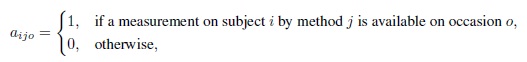
Longitudinal data typically arise in method comparison studies when a cohort of subjects is followed over a period of time and the true value for a subject changes over time. Suppose there are n subjects in the study, labeled as i = 1, ..., n. The two methods being compared are labeled as j = 1, 2. Suppose also that the measurements are to be taken at prespecified time points 1, ..., ![]() . We think of these time points as the values of a discrete quantity called measurement occasion. The study design usually warrants that, for every subject, paired measurements by the two methods are taken on each occasion. In practice, however, there may be some subjects for whom on certain occasions either no measurements are available or a measurement is available from only one of the methods. In particular, suppose mij (≤
. We think of these time points as the values of a discrete quantity called measurement occasion. The study design usually warrants that, for every subject, paired measurements by the two methods are taken on each occasion. In practice, however, there may be some subjects for whom on certain occasions either no measurements are available or a measurement is available from only one of the methods. In particular, suppose mij (≤ ![]() ) repeated measurements are available from method j on subject i. This number may depend on the subject index i as well as the method index j. We use Mi = mi1 + mi2 to denote the total number of observations on the ith subject, and
) repeated measurements are available from method j on subject i. This number may depend on the subject index i as well as the method index j. We use Mi = mi1 + mi2 to denote the total number of observations on the ith subject, and ![]() to denote the total number observations in the dataset.
to denote the total number observations in the dataset.
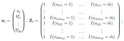
Let Yijk denote the kth repeated measurement from the jth method on the ith subject, and oijk ∈ {1, ..., ![]() } denote the actual occasion on which this measurement is taken, k = 1, ..., mij, j = 1, 2, i = 1, ..., n. Here k represents the order in which the measurements are taken. Each k is associated with a unique measurement occasion in {1, ...,
} denote the actual occasion on which this measurement is taken, k = 1, ..., mij, j = 1, 2, i = 1, ..., n. Here k represents the order in which the measurements are taken. Each k is associated with a unique measurement occasion in {1, ..., ![]() }. It is the value of the occasion index oijk that links the observations taken at the same time. For example, suppose the study design calls for taking four paired measurements from the two methods on each subject every three months, that is,
}. It is the value of the occasion index oijk that links the observations taken at the same time. For example, suppose the study design calls for taking four paired measurements from the two methods on each subject every three months, that is, ![]() = 4. Consider a subject labeled 1 for whom only two measurements are available from method 1—at months 3 and 9, and only three measurements are available from method 2—at months 3, 6, and 9. Here m11 = 2 and m12 = 3. Moreover, k = 1, 2 for method 1 and k = 1, 2, 3 for method 2. Clearly, the index k incorrectly pairs the measurement of method 1 at 9 months with the measurement of method 2 at 6 months. In contrast, for the occasion index we have (o111, o112) = (1, 3) for method 1 and (o121, o122, o123) = (1, 2, 3) for method 2, which implies correct pairings of the measurements.
= 4. Consider a subject labeled 1 for whom only two measurements are available from method 1—at months 3 and 9, and only three measurements are available from method 2—at months 3, 6, and 9. Here m11 = 2 and m12 = 3. Moreover, k = 1, 2 for method 1 and k = 1, 2, 3 for method 2. Clearly, the index k incorrectly pairs the measurement of method 1 at 9 months with the measurement of method 2 at 6 months. In contrast, for the occasion index we have (o111, o112) = (1, 3) for method 1 and (o121, o122, o123) = (1, 2, 3) for method 2, which implies correct pairings of the measurements.
We refer to a subject’s sequence of measurements from a method as a “trajectory.” The data may be called paired longitudinal data in that each subject contributes two dependent trajectories. However, the adjective “paired” here does not necessarily imply both methods are used on each measurement occasion. The modeling of these data generalizes that of linked repeated measurements data of Chapter 5 in two ways. It allows for systematic effect of time and random effect of measurement occasion, whereas only the latter was allowed for linked data. Further, linked data did not allow incomplete pairs of observations, whereas such a restriction is not imposed for longitudinal data.
The effect of time on measurements is taken into account by modeling the means of measurements as functions of time. This involves deciding in the beginning what to take as the “time” covariate because this choice guides how the mean functions are modeled. The time may be a discrete or a continuous covariate depending upon the available data and the interest of the investigator. In either case, let t denote the time covariate of interest and ![]() be its domain. Also, let tijk denote the value of t associated with the measurement Yijk, k = 1, ..., mij, j = 1, 2, i = 1, ..., n. If t represents the measurement occasion, then tijk ≡ oijk and
be its domain. Also, let tijk denote the value of t associated with the measurement Yijk, k = 1, ..., mij, j = 1, 2, i = 1, ..., n. If t represents the measurement occasion, then tijk ≡ oijk and ![]() = {1, ...,
= {1, ..., ![]() }. On the other hand, if t represents a continuous quantity, for example, age of subject, then tijk and oijk are different, and
}. On the other hand, if t represents a continuous quantity, for example, age of subject, then tijk and oijk are different, and ![]() may be taken as the observed range of t in the data.
may be taken as the observed range of t in the data.
Our approach for modeling means as functions of time also allows the within-subject errors of the methods to be correlated over time. The difference in means—a measure of similarity—and measures of agreement that involve them are now functions of time. We assume that two methods are being compared and the errors are homoscedastic. This approach can be extended to deal with more than two methods and heteroscedastic errors along the lines of Chapters 6 and 7. But these extensions are not pursued here.
9.2.1 Displaying Data
The key distinguishing feature of longitudinal data is that the time of measurement has a significant effect. However, it cannot be seen in a trellis plot with one row per subject that we adopted in previous chapters. Therefore, we use method-specific plots of subjects’ trajectories of measurements over time. These plots display all data, including the observations whose paired counterparts are missing. But they do not reveal how close the individual measurements from the two methods are. For this, we can take differences of the paired measurements and plot the trajectories of the differences. These plots can be supplemented with scatterplots, Bland-Altman plots and boxplots of differences for each measurement occasion. Naturally, the plots based on paired measurements use only the complete pairs in the data.
9.2.2 Percentage Body Fat Data
These data come from the Penn State Young Women’s Health Study. They consist of percentage body fat measurements taken by two methods—skinfold caliper (method 1) and dual energy X-ray absorptiometry (DEXA, method 2)—on a cohort of n = 112 adolescent girls whose initial visit occurred around age 12. There are eight subsequent visits roughly six months apart. The visits do not occur at exactly six months for each subject. The measurement occasion variable here is the visit number with possible values 1, ..., 9. The actual age of a subject (in years) is also recorded with each measurement. This age serves as the time covariate of interest. If all nine pairs of measurements were available for each subject, there would have been 112 × 9 × 2 = 2016 observations in the dataset. However, we only have 1515 observations. Of these, 858 are from caliper and 657 are from DEXA. No DEXA observation is available at visit 1. This makes eight the maximum possible value for the number of complete pairs of observations on a subject. A total of 657 complete pairs from 91 subjects are available. Only 37 subjects provide all eight complete pairs. The remaining 75 subjects have observations from one or both methods missing on at least one of the visits. No complete pair is available from 21 subjects. The number of observations per subject averages 7.7 for caliper and 5.9 for DEXA. The ages of the subjects range from 10.7 to 17.3 years, with an average of 13.8 years. The percentage body fat measurements range from 12.7 to 37.4, with an average of 23.5.
Figure 9.1 displays the subjects’ trajectories of body fat measurements over age for caliper and DEXA methods separately. Also superimposed on the plots are the estimated mean functions (see Section 9.5 for details regarding estimation). Both the mean functions fall mostly between 21 and 25, except near the endpoints where the estimates are not reliable, but the means behave differently over age. Roughly speaking, the caliper mean function increases from 22 at age 11 to 25 at age 13.5, decreases thereafter to about 23 at age 15, and increases again to 27 at age 17. On the other hand, the DEXA mean function decreases from 23 at age 11 to 21 at age 13, increases thereafter to just below 25 at age 16, and then shows a slight decline. Figure 9.2 displays the trajectories of DEXA minus caliper differences together with the difference of the fitted mean functions. It appears that, on average, the caliper measurement exceeds its DEXA counterpart except below age 11.5 and between ages 15 and 16 where the situation is slightly reversed. The mean difference decreases from above zero at age 11 to about ‒3 at age 13, increases thereafter to slightly above zero around age 15.5, and then decreases to about ‒2 at age 17. This pattern is also visible in the medians in boxplots of differences at visits two through nine given in Figure 9.3. Figures 9.4 and 9.5, respectively, display scatterplots and Bland-Altman plots of the available pairs at these visits. It is clear that the correlation between the methods remains moderate at all visits. A trend is visible in the Bland-Altman plot at some of the visits, implying potentially unequal scales of the methods, but there is no evidence of heteroscedasticity in the data. Overall, the exploratory analysis suggests that the discrepancy between the means of the methods varies with age. This in turn makes their agreement depend on age. The agreement, nevertheless, does not appear particularly strong. These data are further analyzed in Section 9.5.
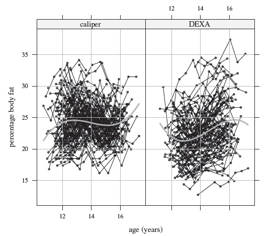
Figure 9.1 Trajectories of percentage body fat measurements for 112 girls. Lines connect the available time points from the same subject. The gray curves in the middle are the estimated mean functions.
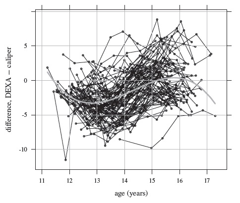
Figure 9.2 Trajectories of DEXA minus caliper differences in percentage body fat measurements for 91 girls with complete measurement pairs. Lines connect the available time points from the same subject. The gray curve in the middle is the estimated mean difference function.
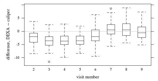
Figure 9.3 Side-by-side boxplots of DEXA minus caliper differences in percentage body fat measurements for visit numbers two through nine, with a reference line at zero.
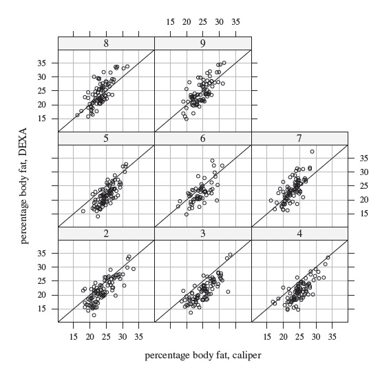
Figure 9.4 Scatterplots of percentage body fat measurements for visit numbers two (bottom left panel) through nine (top right panel). The line of equality is superimposed on each plot.
9.3 MODELING OF DATA
We start with the mixed-effects model (5.9) for linked repeated measurements data and extend it to incorporate effects of time. This involves writing (5.9) in the equivalent form
where ui = bi ‒ μb is the centered true value for subject i as well as method 1, now interpreted as a random effect of subject i common to all observations. Further, (μ1, μ2) = (μb, β0 + μb) are the population means of the two methods. We make three changes to the model while keeping the rest of the assumptions same as before.
First, we allow for the systematic effect of time by replacing the constant mean μj by the mean function μj(t), t ∈ ![]() . This makes μj (t)+ ui as the true value of method j for subject i at time t. The methods are still assumed to be on the same scale because the difference in their true values remains free of ui; but it now depends on t.
. This makes μj (t)+ ui as the true value of method j for subject i at time t. The methods are still assumed to be on the same scale because the difference in their true values remains free of ui; but it now depends on t.

Figure 9.5 Bland-Altman plots of percentage body fat measurements for visit numbers two (bottom left panel) through nine (top right panel) for available pairs. A horizontal line at zero is superimposed on each plot.
Second, we replace the index k in the random effect ![]() of time of measurement with the index oijk to reflect that oijk is the measurement occasion of Yijk. Thus,
of time of measurement with the index oijk to reflect that oijk is the measurement occasion of Yijk. Thus, ![]() is now the random effect of the measurement occasion.
is now the random effect of the measurement occasion.
Third, we allow for the possibility of dependence in the within-subject errors of each method while letting the errors arising from different methods or different subjects remain independent as before. Specifically, we assume that
where h is a specified correlation function, tijk and tijl are the associated times of measurements, and ω is a vector of correlation parameters. The correlation function h(·, ω) is assumed to be continuous in ω, lies between ‒1 and 1, and satisfies the conditions that h(0, ω)= 1 and h(·, 0) = 0. It depends on the measurement times only through their absolute difference, called distance. The time may be discrete, representing, for example, the measurement occasion, or continuous.
The correlation function in (9.1) does not depend on j, that is, the errors from both methods are assumed to follow the same correlation model. This assumption is made to keep the model fitting feasible with existing software capabilities. However, if the fitting is not an issue and the model remains identifiable, the assumption may be relaxed to let the methods have potentially different correlation functions with their own correlation parameters (Exercise 9.4).
9.3.1 The Longitudinal Data Model
The above changes to model (5.9) lead to the following mixed-effects model for longitudinal data:
for i = 1, ..., n, j = 1, 2, k = 1, ..., mij. Here tijk ∈ ![]() are values of the time covariate t of interest and oijk ∈ {1, ...,
are values of the time covariate t of interest and oijk ∈ {1, ..., ![]() } are the measurement occasions. The model makes the following assumptions:
} are the measurement occasions. The model makes the following assumptions:
subject effects ui follow independent
 distributions,
subject × method interactions bij follow independent
 distributions,
subject × occasion interactions
 follow independent
  distributions,
errors eijk follow
 distributions,
errors associated with different subjects or methods are independent, but a method’s errors on the same subject may be dependent following the correlation model (9.1), and
 and eijk are mutually independent.
This model reduces to (5.9) for linked repeated measurements data when μj(t) is free of t, measurements from both methods are available on each occasion, and the correlation parameter ω = 0. Just as in Section 5.4.2, the marginal distributions of the vectors of Mi measurements on subject i = 1, ..., n under (9.2) are independent Mi-variate normal distributions with means and variances
In addition, there are three types of covariances. One is between two measurements of the same method taken at different occasions,
The other two are between measurements from different methods taken at either the same occasion or different occasions. These can be collectively written as
where I is the indicator function, and k, l = 1, ..., mij . We need to specify models for the mean functions μj and the correlation function h to complete the specification of the model (9.2). These issues are discussed in the next two subsections.
Let (Y1(t), Y2(t)) be the paired measurements by the two methods at time t ∈ ![]() on a randomly selected subject from the population. Also, let D(t) = Y2(t) ‒ Y1(t) denote their difference. We need their distributions under the model (9.2) to derive measures of similarity and agreement as functions of t. Proceeding exactly as in Section 5.4.2, we get the companion model for (Y1(t), Y2(t)) as
on a randomly selected subject from the population. Also, let D(t) = Y2(t) ‒ Y1(t) denote their difference. We need their distributions under the model (9.2) to derive measures of similarity and agreement as functions of t. Proceeding exactly as in Section 5.4.2, we get the companion model for (Y1(t), Y2(t)) as
where u, bj, b*, and ej are identically distributed as ![]() , and eijk, respectively. It follows that (Exercise 9.3)
, and eijk, respectively. It follows that (Exercise 9.3)

and
The two distributions depend on t only through the mean functions.
9.3.2 Specifying the Mean Functions
As in Chapter 8, we model the mean functions μ1(t) and μ2(t) as functions of the same form but with different regression parameters. The models depend on whether t is discrete or continuous.
If t is discrete, representing the measurement occasion, then one possibility is to take
It gives each combination of method and measurement occasion its own fixed intercept. This model is equivalent to a fixed-effects model that has a common intercept, main effects of methods and measurement occasions, and the method × occasion interaction effect.
If t is continuous, we proceed exactly as in a regression model and express μj(t) as a parametric function of t (or a suitable transformation thereof) that is linear in regression coefficients. For example, μj (t) may be taken as a polynomial in t of a given degree q,
with unknown method-specific coefficients. Of course, other functional forms can be chosen. The choice is guided by the exploratory analysis of the data. Besides, one has to perform model diagnostics to justify the assumed form.
9.3.3 Specifying the Correlation Function
We now discuss some models for correlation function h of within-subject errors, defined by (9.1). If h is a nonzero constant, the errors are said to follow a model with compound symmetry. Under this model, each error has the same variance and each pair of errors has the same correlation regardless of the distance between the observations (Exercise 9.2). This model may be reasonable if the study period is short. It may be unrealistic for long study periods because the correlation may wear out over time.
Besides the model with compound symmetry (or equal correlation), two classes of models are common within the framework of mixed-effects models—time series and spatial correlation models. They are, respectively, used in the analysis of time series and spatial data.
9.3.3.1 Time Series Correlation Models
The time series models generally require discrete times and work with data that are equally spaced in time. The associated correlation function is called the autocorrelation function and the distance is called lag—a discrete quantity. To specify a correlation function, one may examine the sample autocorrelation function of standardized residuals of the model fit assuming independent errors. Let ![]() denote the residuals and let
denote the residuals and let ![]() denote their standardized counterparts. The sample autocorrelation at lag r for errors of method j can be defined as
denote their standardized counterparts. The sample autocorrelation at lag r for errors of method j can be defined as
where
and
is the number of nonzero terms in the sum in the numerator. The autocorrelation at lag zero is 1 by definition. If the features of ![]() and
and ![]() are similar to those of the autocorrelation function h of a known correlation model, this h can be used to specify the autocorrelation.
are similar to those of the autocorrelation function h of a known correlation model, this h can be used to specify the autocorrelation.
A simple but especially useful time series correlation model is the autoregressive model of order one, denoted as AR(1). It has a single correlation parameter ω. If the time is discrete, its autocorrelation function at lag r is
where ω represents the lag-1 correlation and lies between ‒1 and 1. This correlation function also happens to have a simple analog for continuous times,
where the distance r is continuous, and ω is between 0 and 1. In either case, this model’s characteristic feature is that in absolute terms its correlation function decreases at an exponential rate as the distance r increases. Time series models other than the AR(1) usually do not have simple continuous time analogs for autocorrelation.
9.3.3.2 Spatial Correlation Models
The spatial correlation models are generally specified in terms of semivariograms. Let ![]() denote the standardized errors of a model. These have zero means and unit standard deviations. Their semivariogram is defined as var
denote the standardized errors of a model. These have zero means and unit standard deviations. Their semivariogram is defined as var ![]() . It can be expressed as
. It can be expressed as
relating it with correlation between the standardized errors. Letting s denote a semivariogram function, we can write from (9.1) that
Thus, it follows that a model for the correlation function h may be specified in terms of a model for the semivariogram function s. The properties of h imply that s is continuous in the correlation parameter ω, equals 1 when ω = 0, and satisfies s(0, ω) = 0. The distances |tijk ‒ tijl| in (9.15) can be discrete but they are usually continuous. Although we are using the same correlation parameter ω on both sides of (9.15), it may not have the same interpretation under the two models.
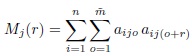
A spatial correlation model for errors in a longitudinal data model may be specified by examining the semivariograms estimated using the standardized residuals ![]() of the model fit assuming independent errors. The semivariogram function for method j can be estimated by
of the model fit assuming independent errors. The semivariogram function for method j can be estimated by
where Mj(r) is the number of terms in the triple sum in the numerator, and
is the index set that identifies the residual pairs associated with subject i and method j that are apart by distance r. The estimates in (9.16) may not be stable if r is a continuous quantity. In this case, we obtain more stable estimates by splitting the range of r into, say, 20 intervals using the quantiles of r, and averaging the semivariogram values over each interval. Just like the time series case, the features of these estimated semivariogram functions may be matched to those of the semivariogram function of a known model to come up with an adequate spatial correlation model.
A popular spatial correlation model is the exponential model, whose semivariogram function is
where ω > 0. In this case, s(r, 0) is not defined, but s(r, ω) converges to 1 as ω tends to 0. By taking ![]() , we get
, we get
and from (9.15), we have ![]() . It follows from (9.13) that the exponential model with correlation parameter ω is equivalent to the continuous AR(1) model with correlation parameter
. It follows from (9.13) that the exponential model with correlation parameter ω is equivalent to the continuous AR(1) model with correlation parameter ![]() .
.
Now that we are familiar with some basic correlation models for errors, a natural question is whether to opt for a time series or a spatial correlation model. The answer is dictated by the time covariate t of interest and whether the data are equally spaced in time. If t represents the measurement occasion, a discrete quantity, and the data are equally spaced, a time series model may be used. If t is a continuous quantity or the data are unequally spaced, a spatial correlation model would be appropriate. Regardless of how a model is chosen, its adequacy must be verified using model diagnostics.
We note from (9.4) that there is an interplay between the correlation structure of the errors and the subject × method interaction effect bij because both induce correlations between a method’s repeated measurements on a subject. Specifying a correlation structure for errors may obviate the need for the bij term in the model, which can be assessed using a test of hypothesis or a model selection criterion (see Section 9.3.4). Alternatively, if the bij term is kept in the model, there may not be any need to model dependence in errors (Exercise 9.2).
9.3.4 Model Fitting and Evaluation
Fitting the model (9.2) involves computing the log-likelihood function of the data and maximizing it numerically with respect to the model parameters using a statistical software package (see Section 9.7 for some technical details). This yields ML estimates of parameters and predicted values of random effects. The fitted values are
where ![]() is the estimated mean function. In particular, when the means are modeled as the polynomial in (9.10), the estimated mean functions are
is the estimated mean function. In particular, when the means are modeled as the polynomial in (9.10), the estimated mean functions are
The raw and standardized residuals of the fitted model are ![]() and
and ![]() , respectively. These quantities can be used in the usual manner for model checking if the within-subject errors are not correlated. If they are, the normalized residuals are used for model checking instead of the standardized residuals (Section 3.2.4).
, respectively. These quantities can be used in the usual manner for model checking if the within-subject errors are not correlated. If they are, the normalized residuals are used for model checking instead of the standardized residuals (Section 3.2.4).
The independence assumption for within-subject errors of the two methods can be verified using plots of the sample autocorrelation functions (9.11) and the estimated semivariogram functions (9.16). If the errors of method j are independent, then approximately 100(1 ‒ α)% of their sample autocorrelations for r > 0 should fall within the bounds
Thus, the independence assumption may not be reasonable if quite a few of the sample autocorrelations fall outside these bounds. The same conclusion is reached if the estimated semivariogram functions do not appear to be a constant. To judge the adequacy of the fitted correlation model, we can use the same approach but with normalized instead of standardized residuals.
A likelihood ratio test can also be performed to test for independence of errors. Under the correlation model (9.1), independence amounts to setting the correlation parameter ω = 0. Therefore, the hypotheses to be tested are
The test statistic (3.32) is obtained by fitting the model with and without the correlation. The degrees of freedom for the test is the number of elements in ω. Alternatively, the two models can be compared with AIC or BIC (Section 3.3.7). These criteria can also be used to compare candidate correlation function models.
As mentioned at the end of Section 9.3.3.2, incorporating a correlation structure in the errors may render the random interaction effect bij in model (9.2) unnecessary. Removing it from the model is equivalent to setting its variance ![]() . Thus, we can assess the need for an interaction term by testing
. Thus, we can assess the need for an interaction term by testing
using a likelihood ratio test. The test statistic (3.32) is obtained by fitting the model with and without the random effect and it has 1 degree of freedom. This test, however, is conservative (see Section 3.3.7).
9.4 EVALUATION OF SIMILARITY AND AGREEMENT
The longitudinal data counterparts of the measures of similarity and agreement are obtained by using the distributions (Y1(t), Y2(t)) and D(t) given by (9.7) and (9.8) in their definitions (Exercise 9.3). For example, the difference in fixed biases at time t is the mean difference ξ(t)= μ2(t) ‒ μ1(t). Likewise, the agreement at time t is measured by
and
The precision ratio λ does not depend on t.
The ML estimators of these measures are obtained in the usual way by replacing the unknowns with their estimators. For inference on measures that depend on t, we need their simultaneous confidence bands over the domain ![]() . In particular, we need a two-sided confidence band for the similarity measure ξ(t), and one-sided confidence bands for agreement measures—a lower band for CCC(t) and an upper band for TDI(t, p). Section 3.3.5 discusses the construction of a simultaneous confidence band for a parametric function over a finite number of points. That methodology is directly applied here if t is discrete because, in this case,
. In particular, we need a two-sided confidence band for the similarity measure ξ(t), and one-sided confidence bands for agreement measures—a lower band for CCC(t) and an upper band for TDI(t, p). Section 3.3.5 discusses the construction of a simultaneous confidence band for a parametric function over a finite number of points. That methodology is directly applied here if t is discrete because, in this case, ![]() = {1, ...,
= {1, ..., ![]() } has a finite set of points. We apply it for continuous t as well by discretizing
} has a finite set of points. We apply it for continuous t as well by discretizing ![]() into a grid of a moderately large number of points, say, 20—30. As before, the confidence bands are initially obtained for the Fisher’s z-transformation of the CCC function and the log transformation of the TDI function. The bands are then transformed back to the original scale (see also Section 9.7). It follows from the distribution of D(t) in (9.8) that the 95% limits of agreement as a function of t are
into a grid of a moderately large number of points, say, 20—30. As before, the confidence bands are initially obtained for the Fisher’s z-transformation of the CCC function and the log transformation of the TDI function. The bands are then transformed back to the original scale (see also Section 9.7). It follows from the distribution of D(t) in (9.8) that the 95% limits of agreement as a function of t are
If the model (9.2) without the interaction bij is adopted, the corresponding agreement measures and their estimates are obtained by simply setting ![]() in their expressions. From (9.22) and (9.23), we obtain (Exercise 9.5)
in their expressions. From (9.22) and (9.23), we obtain (Exercise 9.5)
and
In a similar manner, we get the 95% limits of agreement from (9.24) as
9.5 CASE STUDY
We now return to the percentage body fat data introduced in Section 9.2.2. Our first task is to find an adequate model of the form (9.2). The observed age range in the data, (10.7, 17.3) years, is taken to be the time interval ![]() . After a preliminary analysis, we decide to model the mean functions as cubic functions of age, that is, use the form (9.10) with q = 3. Initially, the model (9.2) is fit with method × subject interaction and independent within-subject errors for the two methods. These data are not equally spaced in time because not every subject is measured on each measurement occasion. Therefore, to explore models for correlation structure we take age as a continuous time variable and examine the semivariograms for the two methods as functions of age difference, representing the “distance.” Figure 9.6 plots the averages of estimated semivariograms (9.16) against the midpoints of various distance intervals. The estimates are computed using standardized residuals of the model with independent errors. The caliper (method 1) semivariogram shows an increasing trend throughout. The DEXA (method 2) semivariogram first shows an increasing trend up to 2 years, and then stabilizes around 0.7. These trends unequivocally suggest that the within-subject errors of the methods should not be regarded as independent. They also indicate that the dependence may be modeled using a continuous AR(1) structure (9.13), which is equivalent to the exponential correlation model (9.17).
. After a preliminary analysis, we decide to model the mean functions as cubic functions of age, that is, use the form (9.10) with q = 3. Initially, the model (9.2) is fit with method × subject interaction and independent within-subject errors for the two methods. These data are not equally spaced in time because not every subject is measured on each measurement occasion. Therefore, to explore models for correlation structure we take age as a continuous time variable and examine the semivariograms for the two methods as functions of age difference, representing the “distance.” Figure 9.6 plots the averages of estimated semivariograms (9.16) against the midpoints of various distance intervals. The estimates are computed using standardized residuals of the model with independent errors. The caliper (method 1) semivariogram shows an increasing trend throughout. The DEXA (method 2) semivariogram first shows an increasing trend up to 2 years, and then stabilizes around 0.7. These trends unequivocally suggest that the within-subject errors of the methods should not be regarded as independent. They also indicate that the dependence may be modeled using a continuous AR(1) structure (9.13), which is equivalent to the exponential correlation model (9.17).
Next, we revise the initial model by assuming a continuous AR(1) structure for within-subject errors with ω as the common correlation parameter for both methods. The likelihood ratio test of the correlation hypotheses (9.20) has a p-value under 0.001, confirming the need for incorporating dependence. Further, to assess whether the subject × method interaction becomes redundant under this correlation model, we perform a likelihood ratio test of (9.21). It has a p-value of 0.18, indicating that the interaction bij in (9.2) may indeed be dropped. Hence, from now on we focus on this model without the interaction term. However, all key conclusions remain unchanged if the interaction is kept in the model (Exercise 9.8).
Table 9.1 provides ML estimates of model parameters, their standard errors, and 95% confidence intervals. The variance-covariance parameters are reparameterized to have unconstrained parameter spaces. None of the standard errors appears unduly large. The correlation parameter ω is estimated as 0.54 with (0.48, 0.61) as its 95% confidence interval. The adequacy of the assumed continuous AR(1) correlation structure can be checked by examining either the sample autocorrelation functions (9.11) of normalized residuals under the fitted model, or the estimated semivariograms (9.16). The latter are left for Exercise 9.7. The autocorrelation functions are presented in Figure 9.7. As there are nine visits by design, we expect autocorrelations at lags one through eight. However, DEXA’s autocorrelations are available only through lag seven because its measurements are missing from the first visit. Also plotted in the figure are the bounds (9.19) with α =0.05. The bounds increase with lag, in absolute value terms, because they are computed using fewer observation pairs as the lag increases. Only one autocorrelation falls outside the bounds, that too barely, suggesting that the assumed correlation structure may be considered adequate. Further model adequacy checking is pursued in Exercise 9.7. It also explores other degrees for the polynomial mean functions. In particular, the model with constant means β0j has a p-value under 0.001, justifying the need for letting the means be functions of age. This exercise additionally explores other spatial correlation models for errors. Overall, the model (9.2) with cubic mean functions and continuous AR(1) errors but without the subject × method interaction appears to provide an adequate fit.
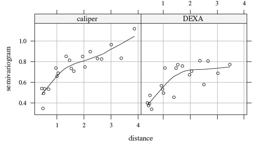
Figure 9.6 Estimated semivariogram functions for caliper and DEXA methods computed using standardized residuals from a model fit to percentage body fat data with independent within-subject errors. A nonparametric smooth curve is added to each plot to show the underlying trend.
From (9.7), (9.8), and Exercise 9.5, the distributions of (Y1(t), Y2(t)) and D(t) for t ∈ ![]() under the fitted model are
under the fitted model are

Here ![]() and
and ![]() are the fitted mean functions given by (9.18) using the estimates given in Table 9.1. They and their difference
are the fitted mean functions given by (9.18) using the estimates given in Table 9.1. They and their difference ![]() were shown as gray curves in Figures 9.1 and 9.2. The mean difference is also plotted in Figure 9.8. The caliper’s mean is lower than DEXA’s for young women below age 11.5 and it is higher in the age range (11.5, 14.5). Their values are similar beyond age 14.5. With the exception of the left endpoint of
were shown as gray curves in Figures 9.1 and 9.2. The mean difference is also plotted in Figure 9.8. The caliper’s mean is lower than DEXA’s for young women below age 11.5 and it is higher in the age range (11.5, 14.5). Their values are similar beyond age 14.5. With the exception of the left endpoint of ![]() , the mean difference function is less than 3.5 in absolute value. From (9.28), the correlation between the methods is about 0.7. One reason why this correlation is not very high is that the error variations are not very small relative to the between-subject variation. The standard deviation of the difference is about 3.1. This variability is solely attributed to the error variations of the methods. The 95% limits of agreement as functions of age, given by (9.27), are also plotted in Figure 9.8. The lower and the upper limits range between ‒9.5 and ‒0.9 and 2.7 and 11.3, respectively. They indicate rather weak agreement between the methods on most of
, the mean difference function is less than 3.5 in absolute value. From (9.28), the correlation between the methods is about 0.7. One reason why this correlation is not very high is that the error variations are not very small relative to the between-subject variation. The standard deviation of the difference is about 3.1. This variability is solely attributed to the error variations of the methods. The 95% limits of agreement as functions of age, given by (9.27), are also plotted in Figure 9.8. The lower and the upper limits range between ‒9.5 and ‒0.9 and 2.7 and 11.3, respectively. They indicate rather weak agreement between the methods on most of ![]() . The limits have a constant width because the standard deviation of the difference does not depend on age.
. The limits have a constant width because the standard deviation of the difference does not depend on age.
Table 9.1 Summary of estimates of model parameters for percentage body fat data. Methods 1 and 2 refer to caliper and DEXA, respectively.


Figure 9.7 Sample autocorrelation functions for normalized residuals of caliper and DEXA methods under a model fit to percentage body fat data with AR(1) errors. The dashed curves represent the 95% bounds (9.19).
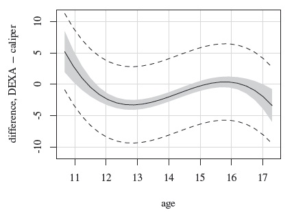
Figure 9.8 Estimate of mean difference in percentage body fat using caliper and DEXA methods (solid curve), its 95% two-sided simultaneous confidence band (shaded region), and the 95% limits of agreement (broken curves).
We proceed next to the evaluation of similarity. Figure 9.8 presents estimate of the mean difference along with its 95% two-sided simultaneous confidence band. This as well as the other simultaneous bands reported here are computed on a grid of 25 equally spaced points in ![]() . The critical point for the band in Figure 9.8 is 2.67. As is often the case in practice, this band is widest near the endpoints because there is not much data near the extremes. The zero line falls within the band except near the endpoints and also when the age is roughly between 11.5 and 14.5, in which case the band is below the line. Thus, the means of the two methods cannot be considered equal over the entire age interval. In particular, the caliper’s estimated mean percentage body fat exceeds that of DEXA’s by about 2—3 between the ages of 11.5 and 14.5. The precision ratio λ is estimated as 1.30 with (1.06, 1.58) as its 95% confidence interval. Clearly, DEXA appears more precise than caliper. Taken together, these findings suggest that the methods cannot be regarded as similar.
. The critical point for the band in Figure 9.8 is 2.67. As is often the case in practice, this band is widest near the endpoints because there is not much data near the extremes. The zero line falls within the band except near the endpoints and also when the age is roughly between 11.5 and 14.5, in which case the band is below the line. Thus, the means of the two methods cannot be considered equal over the entire age interval. In particular, the caliper’s estimated mean percentage body fat exceeds that of DEXA’s by about 2—3 between the ages of 11.5 and 14.5. The precision ratio λ is estimated as 1.30 with (1.06, 1.58) as its 95% confidence interval. Clearly, DEXA appears more precise than caliper. Taken together, these findings suggest that the methods cannot be regarded as similar.
For agreement evaluation, Figure 9.9 displays estimates of CCC and TDI with p =0.90 as functions of age, defined by (9.25) and (9.26), respectively. The estimates near the endpoints cannot be trusted because of their relatively high standard errors. Also presented are their 95% one-sided simultaneous confidence bands over ![]() . The critical points used for CCC and TDI bands are ‒2.27 and 2.47, respectively. Both measures show essentially the same pattern of change in the extent of agreement with age: increase from the beginning till about age 11.5, then decrease till about age 13, then increase again till about age 14.5, remain constant near the peak till about age 16.5, and decrease again thereafter. This behavior appears to be driven by the behavior of the estimated mean difference function in Figure 9.8. In particular, the age interval (11.5, 14.5) over which the extent of agreement decreases from its initial peak, attains nadir, and eventually peaks again roughly coincides with the interval over which DEXA’s mean is significantly lower than the caliper’s mean. The agreement is best around age 11.5 and between the ages of 14.5 and 16.5. It is worst around age 13. There may be a physiological explanation of this phenomenon that is tied to how the two methods measure percentage body fat in adolescent women.
. The critical points used for CCC and TDI bands are ‒2.27 and 2.47, respectively. Both measures show essentially the same pattern of change in the extent of agreement with age: increase from the beginning till about age 11.5, then decrease till about age 13, then increase again till about age 14.5, remain constant near the peak till about age 16.5, and decrease again thereafter. This behavior appears to be driven by the behavior of the estimated mean difference function in Figure 9.8. In particular, the age interval (11.5, 14.5) over which the extent of agreement decreases from its initial peak, attains nadir, and eventually peaks again roughly coincides with the interval over which DEXA’s mean is significantly lower than the caliper’s mean. The agreement is best around age 11.5 and between the ages of 14.5 and 16.5. It is worst around age 13. There may be a physiological explanation of this phenomenon that is tied to how the two methods measure percentage body fat in adolescent women.
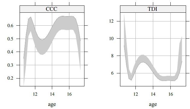
Figure 9.9 Estimates of CCC and TDI functions (solid curves) and their 95% one-sided simultaneous confidence bands (shaded regions) for percentage body fat data.
It is evident that even in the best case scenario, the agreement between caliper and DEXA methods is not high enough for interchangeable use. For example, the largest value of CCC lower bound is 0.60, which may only be considered modest. Further, the smallest value of TDI upper bound is 5.5, which is about 23% of the average body fat measurement in the data, a particularly large value. Besides a difference in their means, the lack of agreement is also due to the relatively large error variations of the methods that lead to a somewhat low correlation between them and a high standard deviation for their difference. The latter issues cannot be addressed by a simple recalibration of the methods. DEXA may be preferred because of its higher precision than the skinfold caliper.
9.6 CHAPTER SUMMARY
- A methodology for analysis of longitudinal method comparison data is presented. It generalizes the one for linked repeated measurements data and allows systematic effects of time on measurements (Chapter 5).
- Time covariate may be discrete or continuous.
- Means of the methods are modeled using functions of time of the same form but with method-specific parameters.
- If time is discrete, each of its levels is given its own intercept.
- If time is continuous, its effect is modeled as in regression analysis with a continuous predictor.
- The extent of agreement between the methods may change over time.
- The model does not require observations from both methods on every measurement occasion.
- The model allows dependence in the within-subject errors of the same method. The errors of different methods are assumed independent.
- Time series or spatial correlation models can be used to model dependence in the within-subject errors.
- By default, the model has a subject × method interaction term. However, it may not be needed when the errors are assumed to be correlated.
- Simultaneous confidence bands are used for measures that depend on time.
- The methodology assumes a common scale for the methods and is applicable when the number of subjects is large.
9.7 TECHNICAL DETAILS
First, we focus on the general model (9.2) that includes subject × method interaction.
Let ![]() vector of measurements from method j on subject i, and
vector of measurements from method j on subject i, and ![]() be the corresponding
be the corresponding ![]() vector of random errors. Define
vector of random errors. Define
as Mi × 1 vectors of observations and random errors associated with subject i, respectively. Regardless of whether t is discrete or continuous, let βj be the (p + 1) × 1 vector of regression coefficients associated with the mean function of method j and Xij be the corresponding mij × (p + 1) design matrix. Define
respectively, as a 2(p + 1) × 1 vector and a Mi × 2(p + 1) matrix.
Next, let ui be the ![]() vector of random effects involving this subject and Zi be the
vector of random effects involving this subject and Zi be the ![]() design matrix associated with ui. These are defined as
design matrix associated with ui. These are defined as
where oijk ∈ {1, ..., ![]() } is the measurement occasion of Yijk. It is assumed that
} is the measurement occasion of Yijk. It is assumed that
where Rij is an mij ×mij covariance matrix whose (k, l)th element is ![]() , with h as the correlation function defined in (9.1). It reduces to a diagonal matrix when the correlation parameter ω = 0. The random vectors ui and ei are mutually independent.
, with h as the correlation function defined in (9.1). It reduces to a diagonal matrix when the correlation parameter ω = 0. The random vectors ui and ei are mutually independent.
Now, the model (9.2) can be written in matrix notation as
where ui and ei follow the distributions given in (9.30). The vector of transformed model parameters is
The fitting of such a mixed-effects model and associated inference based on the large-sample theory of ML estimators have been described in Chapter 3. Of particular interest is the construction of simultaneous confidence bands for measures that depend on t over its domain ![]() . The methodology of Section 3.3.5 is used for this task.
. The methodology of Section 3.3.5 is used for this task.
To represent the model (9.2) without the interaction, we simply drop (bi1, bi2) from ui in (9.29). Essentially, this amounts to redefining ui and Zi in (9.29) as
redefining G in (9.30) as ![]() , dropping log(ψ2) as an unknown parameter from θ, making the corresponding changes in the estimates, and replacing (
, dropping log(ψ2) as an unknown parameter from θ, making the corresponding changes in the estimates, and replacing (![]() + 3) with (
+ 3) with (![]() + 1) (Exercise 9.5).
+ 1) (Exercise 9.5).
9.8 BIBLIOGRAPHIC NOTE
The topic of longitudinal data analysis has been covered in a number of books, including Diggle et al. (2002) and Fitzmaurice et al. (2011). However, the analysis of longitudinal method comparison data has been considered by only a handful of authors. Chinchilli et al. (1996), King et al. (2007a), and Hiriote and Chinchilli (2011) generalize the usual CCC to obtain overall summary measures for longitudinal data. Specifically, Chinchilli et al. develop subject-specific CCCs under a random-coefficient growth curve model and combine them into an overall weighted CCC. Both King et al. and Hiriote and Chinchilli assume that each subject contributes two ![]() × 1 vectors, consisting of paired measurements by the two methods on each measurement occasion. King et al. develop a “repeated measures” CCC that characterizes how close the two vectors are through a single index. They also incorporate an
× 1 vectors, consisting of paired measurements by the two methods on each measurement occasion. King et al. develop a “repeated measures” CCC that characterizes how close the two vectors are through a single index. They also incorporate an ![]() ×
×![]() weight matrix into the index to allow differential emphasis on within-and between-occasion agreement between the methods. Hiriote and Chinchilli develop a “matrix-based” CCC by first constructing an
weight matrix into the index to allow differential emphasis on within-and between-occasion agreement between the methods. Hiriote and Chinchilli develop a “matrix-based” CCC by first constructing an ![]() ×
× ![]() matrix that measures agreement between the two vectors. Then they transform the matrix into a scalar quantity by taking its Frobenius norm and scaling it to lie between ‒1 and 1. The inference procedures proposed by both King et al. and Hiriote and Chinchilli do not make any assumptions about the correlation structure between the measurements. However, they require measurements from both methods on each measurement occasion. Carrasco et al. (2009) focus on a special case of the repeated measures CCC developed by King et al. but consider likelihood-based inference on the measure by assuming a mixed-effects model for the data. Their model allows missing observations and is a special case of the model we consider here. See Carrasco et al. (2009) and Hiriote and Chinchilli (2011) for comparisons of the various approaches.
matrix that measures agreement between the two vectors. Then they transform the matrix into a scalar quantity by taking its Frobenius norm and scaling it to lie between ‒1 and 1. The inference procedures proposed by both King et al. and Hiriote and Chinchilli do not make any assumptions about the correlation structure between the measurements. However, they require measurements from both methods on each measurement occasion. Carrasco et al. (2009) focus on a special case of the repeated measures CCC developed by King et al. but consider likelihood-based inference on the measure by assuming a mixed-effects model for the data. Their model allows missing observations and is a special case of the model we consider here. See Carrasco et al. (2009) and Hiriote and Chinchilli (2011) for comparisons of the various approaches.
The above articles summarize the extent of agreement in a single CCC-type index. None is concerned with examining how the agreement changes over time, which is a goal of Choudhary (2007). It works with differences in paired longitudinal measurements, models them semiparametrically as a function of time via penalized splines, and measures agreement using TDI as a function of time. It uses a Bayesian approach for inference. Our approach in this chapter is to directly model the paired longitudinal data instead of modeling their differences. This has two advantages. Firstly, we can use all data, whereas working with differences necessitates discarding observations whose paired counterparts are missing—a common occurrence in longitudinal studies. Secondly, we have the additional flexibility of using any measure of agreement we like because it can be expressed in terms of parameters of the model for the entire data.
Our discussion of correlation models for errors is kept quite brief and is primarily based on Pinheiro and Bates (2000). The books by Brockwell and Davis (2002) on time series analysis and Cressie (1993) on spatial statistics detail a variety of correlation models. More focussed discussions in the specific contexts of longitudinal data and mixed-effects models can be found in Pinheiro and Bates (2000), Diggle et al. (2002), and Fitzmaurice et al. (2011). These books also explain diagnostics for checking the adequacy of the fitted correlation models. Quite a few correlation models are implemented in the nlme package of Pinheiro and Bates for fitting mixed-effects models in R. The conservative nature of the likelihood ratio test of zero variance of a random effect is described in Pinheiro and Bates (2000, Section 2.4).
Data Source
The percentage body fat data are from Chinchilli et al. (1996). They have also been analyzed by a number of authors, including Choudhary (2007), King et al. (2007a), and Hiriote and Chinchilli (2011). They can be obtained from the book’s website.
EXERCISES
Consider random variables Y1, ..., Ym with a common mean. They are said to follow a compound symmetric correlation structure if they have a common variance σ2 and a common correlation ρ, that is,

Show that this correlation structure is valid only if ‒1/(m ‒ 1) ≤ ρ ≤ 1. [Hint: Examine the variance of the average
 .]
.]Consider the model (9.2) with errors following independent
 distributions for k = 1, ..., mij , j = 1, 2, i = 1, ..., n.
Define
 , and write the model as
 . Show that for a given (i, j), the new errors
  have a compound symmetric correlation structure with
  as the common variance and
  as the common correlation. (This correlation is an intraclass correlation.)
Write the model in (a) by replacing
 with
with  that follow normal distributions with mean zero and a compound symmetric correlation structure with
  as the common variance and ω as the common correlation. Are the two models equivalent? Justify your answer.
-
Verify that the distributions of (Y1(t),Y2(t)) and D(t) for t ∈
 under the model (9.6) are given by (9.7) and (9.8), respectively.
Use (a) to verify that the longitudinal version of the similarity measure β0 is
 and the longitudinal versions of CCC and TDI are given by (9.22) and (9.23), respectively.
Consider the model (9.2). Replace the assumption of a common correlation function (9.1) for within-subject errors of the two methods with

This allows each method to have its own correlation function as well as correlation parameters. Derive the measures of similarity and agreement under this model.
Consider the model (9.2) without the subject × method interaction bij, that is,

Consider the longitudinal data model (9.2). Derive expressions for CCC and TDI under this model for measuring agreement between an observation from method 1 at time t and an observation from method 2 at time t + Δ, where |Δ| > 0. How do these expressions compare with the case when Δ = 0? (See also King et al., 2007a.)
Consider the percentage body fat data from Section 9.5.
Fit the model (9.2) with cubic mean functions and continuous AR(1) within-subject errors and without the method × subject interaction. Verify the estimates in Table 9.1. Perform diagnostics to check the various model assumptions.
Refit the model in (a) with polynomial mean functions of degree q = 1, 2, 4. Perform model comparison to determine which degree should be used. Would you still recommend q = 3?
Refit the model in (a) with compound symmetric correlation structure for the errors. Does this correlation model provide a better fit than the continuous AR(1) structure?
Reanalyze the body fat data by modeling them using (9.2) with subject × method interaction, and compare conclusions with those obtained in Section 9.5.