CHAPTER 10
A NONPARAMETRIC APPROACH
10.1 PREVIEW
Here we present a nonparametric approach for analysis of continuous method comparison data. Attention is restricted to the evaluation of similarity and agreement. The methodology makes no assumption about either the shape of the data distribution or how the observed measurements are related to the underlying true values. It is an alternative to the normality-based parametric approaches of previous chapters, and is especially attractive for data with marked deviations from normality. It works for unreplicated as well as unlinked repeated measurements data. It takes a statistical functional approach that treats the population quantities, including the measures of similarity and agreement, as features of a population distribution and estimates them using the same features of an empirical distribution. Under certain assumptions, the resulting estimators are approximately normal for large samples. This result is used to develop nonparametric analogs of the procedures in Chapter 7 involving multiple methods. Its application is illustrated using two case studies.
10.2 INTRODUCTION
Consider the setup of Chapter 7. We have measurements from J ( ≥ 2) methods on n subjects. It is assumed that n is large. The measurements may be unreplicated or repeated. The latter are assumed to be unlinked. The unreplicated measurements are denoted by Yij, j = 1,..., J, i = 1,...,n. The repeated measurements are denoted by Yijk, k = 1,..., mij, j = 1 ..., J, i = 1,...,n. In the balanced case when all mij are equal, m denotes the common value. To present a unified framework encompassing both data types, we treat unreplicated data as a special case of repeated measurements data with all mij = 1. Thus, Yij is essentially an alias for Yij1, and m = 1 refers to the unreplicated case. As before, (Y1,...,YJ) denotes the population vector of single measurements from the J methods on the same subject. Let F (y1,...,yJ) be its joint cdf. A cdf is also used to refer to the distribution it characterizes.
The methods used in previous chapters are parametric in that the data are assumed to follow a probability distribution of a known form, specifically a normal distribution, characterized in terms of model parameters. The parameters are estimated by the ML method. Under certain assumptions, the ML estimators are efficient, essentially meaning that, if the assumed model is correct and n is large, one cannot find more accurate estimators than them. This optimality property breaks down if the assumed model is wrong, in which case the ML estimators may be a poor choice. In contrast, the methodology of this chapter is nonparametric or distribution-free in that no particular form is assumed for the data distribution, thereby allowing the methodology to be broadly applicable. However, there is a trade-off. Although a nonparametric estimator may be more accurate than the ML estimator if the assumed model is wrong, the converse is true if the assumed model is correct because of the latter’s efficiency. This motivates the common practice of initially attempting a parametric analysis wherein a normality-based model is first fit, followed by model diagnostics to verify the normality assumption. If no serious violations are seen, one proceeds with the parametric analysis, otherwise a nonparametric analysis is pursued. The violations include skewness and outliers in the data. Often, however, the two analyses produce similar inferences regardless of how serious the violations are.
The nonparametric approach also has limitations brought upon by its assumptions or lack thereof, including the following two that are relevant here. First, it does not decompose the observed values into true values and errors. As a result, the usual characteristics of measurement methods such as biases and precisions considered in Section 1.7, and hence the associated measures of similarity are left undefined. Thus, there is a need for alternative measures. Second, the approach does not generalize well to data with features such as heteroscedasticity and covariate effects that call for explicit modeling. It is easier to analyze such data within a parametric framework.
Notwithstanding its limitations, a nonparametric approach remains useful for analysis of basic types of method comparison data. To describe it, we let

and assume that the distribution of (Y1,...,YJ) is continuous; the measurements on different subjects are independent; and for each i = 1,...,n, the ci possible J -tuples formed by selecting one measurement per method from the available measurements on the ith subject, that is,

are identically distributed as (Y1,...,YJ).
For unreplicated data, there is only one J-tuple per subject. The assumptions imply they are i.i.d. draws from the distribution of (Y1,...,YJ). For repeated measurements data, there are ci J-tuples from the ith subject, resulting in a total of ![]() tuples. These tuples are also identically distributed draws from the distribution of (Y1,...,YJ), but independence holds only for the tuples from different subjects. Those from the same subject are dependent. This also means that a subject’s multiple tuples are treated the same way in that they carry the same amount of information.
tuples. These tuples are also identically distributed draws from the distribution of (Y1,...,YJ), but independence holds only for the tuples from different subjects. Those from the same subject are dependent. This also means that a subject’s multiple tuples are treated the same way in that they carry the same amount of information.
The population moments and functions thereof, viz., means, variances, and correlations, play a key role in the analysis of method comparison data. These quantities are fine for normal data, but one may question their value for non-normal data. Their usage may be considered particularly problematic if the data have outliers because the nonparametric estimators of population moments are sample moments, which are not robust to outliers. However, a discussion of robust alternatives to moments and measures based on them is beyond the scope of this book (see Bibliographic Note for a reference). Instead, if outliers are seen in the data, then as in a parametric approach, we perform the analysis twice—with and without the outliers—and compare the conclusions. The analysis also involves inference on percentiles. But their nonparametric estimators are relatively more robust to outliers than those of moments.
10.3 THE STATISTICAL FUNCTIONAL APPROACH
This approach is a general method for constructing nonparametric estimators. It treats the population quantities as statistical functionals, that is, functions of the form h(F), where h is a known function and F is the population cdf. Writing a population quantity in this way highlights it as a feature h of the population distribution F. The cdf F is estimated nonparametrically by the empirical cdf ![]() . Thereafter, F in h(F) is replaced by
. Thereafter, F in h(F) is replaced by ![]() to get the plug-in estimator h(
to get the plug-in estimator h(![]() )—the same feature h of the sample distribution
)—the same feature h of the sample distribution ![]() . This estimator may be considered a “natural” estimator for h(F). Parameters such as population moments and percentiles and functions thereof are readily written as statistical functionals (Exercise 10.1), and their sample analogs can be thought of as plug-in estimators (Exercise 10.2).
. This estimator may be considered a “natural” estimator for h(F). Parameters such as population moments and percentiles and functions thereof are readily written as statistical functionals (Exercise 10.1), and their sample analogs can be thought of as plug-in estimators (Exercise 10.2).
For a concrete example, consider the population mean µj of the jth measurement method. The feature h here is the mean of the jth component of the distribution F of (Y1,...,YJ). From unreplicated data, F can be estimated by the empirical cdf,
 (10.1)
where I(A) is the indicator function of an event A, defined as
It is readily seen that the mean of the jth component of the distribution ![]() is the sample mean
is the sample mean ![]() (Exercise 10.2). Thus, we have the anticipated result that the sample mean is a plug-in estimator of the population mean.
(Exercise 10.2). Thus, we have the anticipated result that the sample mean is a plug-in estimator of the population mean.
10.3.1 A Weighted Empirical CDF
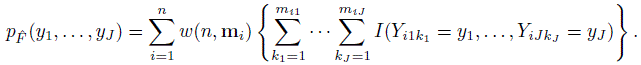
It is clear that we need a nonparametric estimator ![]() of F to construct plug-in estimators of population quantities. For unreplicated data, the empirical cdf (10.1) is a natural choice. But no such candidate is apparent for repeated measurements data in general. Here we focus on a weighted generalization of (10.1) of the form:
of F to construct plug-in estimators of population quantities. For unreplicated data, the empirical cdf (10.1) is a natural choice. But no such candidate is apparent for repeated measurements data in general. Here we focus on a weighted generalization of (10.1) of the form:
 (10.2)
where w is a weight function; mi = (mi1,...,miJ)T; and {(Yi1k1,...,YiJkJ), kj = 1,..., mij, j = 1,..., J} are the ci J-tuples formed by the measurements on the ith subject. The J-tuples from a subject receive the same weight. The weight depends on the number of replications on the subject and not on (Y1,...,YJ). The weight function is non-negative and is assumed to satisfy an unbiasedness condition,
 (10.3)
so that ![]() is an unbiased estimator of F.
is an unbiased estimator of F.
When the design is balanced with all mij = m, the weight function in (10.2) does not depend on the subject index. In fact, in this case ci is a constant and the unique weight function satisfying (10.3) is the constant function
 (10.4)
It gives equal weight to all J-tuples in the data. Due to its uniqueness, the resulting ![]() may be considered a “standard” empirical cdf for balanced designs. Besides, when m = 1, it reduces to the cdf (10.1) for unreplicated data. Therefore, hereafter we use (10.4) as the weight function for unreplicated as well as balanced repeated measurements data.
may be considered a “standard” empirical cdf for balanced designs. Besides, when m = 1, it reduces to the cdf (10.1) for unreplicated data. Therefore, hereafter we use (10.4) as the weight function for unreplicated as well as balanced repeated measurements data.
For unbalanced data, we focus on two candidate weight functions. They are
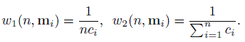 (10.5)
The first gives equal weight to each subject i in the data and distributes that weight equally over all its ci J-tuples. The second gives equal weight to all the J-tuples in the entire dataset. These two are extreme but useful special cases of an optimal weight function (Exercise 10.6). All these weight functions reduce to (10.4) for balanced designs. Thus, choosing between w1 and w2 is an issue only for unbalanced designs. In this case, we suggest analyzing data using both of them and comparing the conclusions because neither is a uniformly better choice than the other (see Bibliographic Note).
10.3.2 Distributions Induced by Empirical CDF
The cdf ![]() in (10.2) induces a discrete multivariate empirical distribution for (Y1,...,YJ), whose possible values are the observed
in (10.2) induces a discrete multivariate empirical distribution for (Y1,...,YJ), whose possible values are the observed ![]() J-tuples in the dataset. Despite the fact that the underlying population distribution is continuous, there may be ties among a method’s measurements and hence among the J-tuples. Allowing for the possibility of ties, the joint probability mass function (pmf) of (Y1,...,YJ) under
J-tuples in the dataset. Despite the fact that the underlying population distribution is continuous, there may be ties among a method’s measurements and hence among the J-tuples. Allowing for the possibility of ties, the joint probability mass function (pmf) of (Y1,...,YJ) under ![]() is
is
 (10.6)
The notation p![]() emphasizes that the pmf is associated with the distribution
emphasizes that the pmf is associated with the distribution ![]() . The inner sum on the right in (10.6) essentially counts the frequency of (y1,...,yJ) among each subject’s tuples. A weighted sum of these frequencies is the probability of observing (y1,...,yJ). Upon summing (10.6) over the remaining components, we get the joint pmf of (Yj, Yl), j ≠ l as
. The inner sum on the right in (10.6) essentially counts the frequency of (y1,...,yJ) among each subject’s tuples. A weighted sum of these frequencies is the probability of observing (y1,...,yJ). Upon summing (10.6) over the remaining components, we get the joint pmf of (Yj, Yl), j ≠ l as
 (10.7)
and the marginal pmf of Yj as
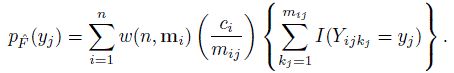 (10.8)
The expressions for these pmfs are verified in Exercise 10.3. Their special cases when there are no within-method ties are derived in Exercise 10.4 for unbalanced designs and in Exercise 10.5 for balanced designs.
Now that we have the pmfs (10.7) and (10.8) under ![]() , we can compute certain moments and percentiles involving (Yj, Yl) by simply invoking their definitions. They serve as plug-in estimators of their population analogs under F. In particular, the estimators of first-and second-order moments are
, we can compute certain moments and percentiles involving (Yj, Yl) by simply invoking their definitions. They serve as plug-in estimators of their population analogs under F. In particular, the estimators of first-and second-order moments are
 (10.9)
As before, the notation E![]() emphasizes that the expectation is associated with the distribution
emphasizes that the expectation is associated with the distribution ![]() . It follows that the corresponding estimators of means and variances of Yj and Yl and their correlation are
. It follows that the corresponding estimators of means and variances of Yj and Yl and their correlation are
 (10.10)
These estimators can also be used in the usual manner to get the corresponding estimators of mean and variance of the difference Djl = Yl − Yj.
Next, let Gjl be the cdf of | Djl |. It can be written as an expectation as

Hence its plug-in estimator is
 (10.11)
Exercise 10.8 gives alternative expressions for the estimators in (10.9) and (10.11); those may be simpler to evaluate. The 100 γth percentile of | Djl | is defined as the inverse cdf ![]() wher
wher

Its sample counterpart ![]() is also similarly defined, that is,
is also similarly defined, that is,
 (10.12)
10.4 EVALUATION OF SIMILARITY AND AGREEMENT
The nonparametric approach of this chapter does not make any assumptions about: (a) the shape of the data distribution, and (b) how the observed measurements are related to the true values. Although this does not pose any difficulty with measures of agreement such as CCC and TDI, the limits of agreement discussed earlier are not meaningful anymore because their definition is tied to normality of data. In addition, (b) precludes us from defining measures of similarity such as the difference in fixed biases and ratio of precisions. A similar situation occurred in Chapter 4 for paired measurements data when we switched from the mixed-effects model (4.1) to the bivariate normal model (4.6). However, as in that chapter, the similarity of two methods can be examined by directly comparing their means and variances using mean difference and variance ratio, respectively.
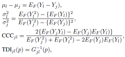
Just like Chapter 7, suppose there are Q specified pairwise comparisons of interest involving the J methods in the study. The population vector of their measurements is (Y1,...,YJ). Its cdf F is estimated by the weighted empirical cdf ![]() given in (10.2) with weights given by (10.4) for balanced designs and by (10.5) for unbalanced designs. For a method pair ( j, l), j < l = 1,..., J of interest, the measures of similarity are the mean difference µl − µj and the variance ratio σ2l /σ2j. Moreover, the measures of agreement are CCCjl and TDIjl(p). These measures are statistical functionals of the distribution F (Exercise 10.7). The plug-in estimators of the similarity measures are
given in (10.2) with weights given by (10.4) for balanced designs and by (10.5) for unbalanced designs. For a method pair ( j, l), j < l = 1,..., J of interest, the measures of similarity are the mean difference µl − µj and the variance ratio σ2l /σ2j. Moreover, the measures of agreement are CCCjl and TDIjl(p). These measures are statistical functionals of the distribution F (Exercise 10.7). The plug-in estimators of the similarity measures are ![]() and those of the agreement measures are
and those of the agreement measures are
 (10.13)
where the quantities involved are given by (10.9) and (10.12).
Thus, we have nonparametric estimators of measures of similarity and agreement for each of the Q pairs of interest. Under certain assumptions, these plug-in estimators are approximately normal from the large-sample theory of statistical functionals, and their SEs can be approximated using estimated moments of influence functions (see Section 10.7). As in Chapter 7, we examine Q two-sided simultaneous confidence intervals for a similarity measure, and Q one-sided simultaneous confidence bounds for an agreement measure. These are of the usual form
 (10.14)
possibly on a transformed scale. Specifically, a log transformation is applied for the variance ratios and a Fisher’s z-transformation is applied for the CCCs. One exception to (10.14) is TDI for which upper confidence bounds of the following from is suggested (Section 10.7):
 (10.15)
These bounds avoid the estimation of the pdf of | Djl | in the tails, which is needed for the bounds in (10.14). Such density estimates are generally not stable unless n is quite large. The critical points are N1(0, 1) percentiles when Q = 1. For Q > 1, they are computed numerically as described in Section 3.3 (see also Section 10.7).
Two observations are now in order about the nonparametric estimators of means, variances, and correlation of Yj and Yl given by (10.10). First, in the case of unreplicated data with J = 2, these estimators are identical to the ML estimators given by (4.8) under the bivariate normal model (4.6) (Exercise 10.2). Second, in the case of balanced repeated measurements data, the estimators in (10.10) often tend to be close to the ML estimators under the mixed-effects model (7.7). Consequently, the nonparametric and the ML estimators of the moment-based measures, ![]() and CCCjl, coincide in the first case and tend to be close in the second case.
and CCCjl, coincide in the first case and tend to be close in the second case.
10.5 CASE STUDIES
In this section, we illustrate the nonparametric methodology by using it to analyze two datasets. Both consist of measurements of systolic blood pressure (mm Hg), but the first has unreplicated observations from two methods, whereas the second has replicated observations from three methods. For convenience, we refer to the first as “unreplicated blood pressure data” and the second as “replicated blood pressure data.”
10.5.1 Unreplicated Blood Pressure Data
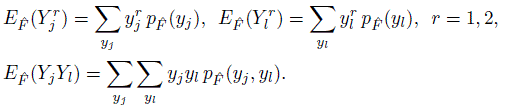
This dataset has paired blood pressure measurements of 200 subjects taken by a standard method using arm pressure (method 1) and a test method using finger pressure (method 2). There is a total of 200 × 2 = 400 observations in the data. They range between 60 and 228 mm Hg. Figure 10.1 shows their trellis plot. The measurements from the two methods do not have much overlap. The finger’s measurements exceed their arm counterparts for most subjects. The former also exhibit somewhat larger variability than the latter. A handful of subjects have relatively large differences, suggesting that the differences have a skewed distribution. However, there are no clear outliers. There is considerable within-subject variation in the measurements, but this variation is small in relation to the between-subject variation. The data can be considered homoscedastic. The scatterplot in Figure 10.2 shows modest correlation in the methods. The Bland-Altman plot in the same figure shows a mild upward trend, corroborating the somewhat unequal variances of the methods. This trend may also be indicative of unequal scales of the methods but we cannot be sure due to lack of replications. The boxplots in Figure 10.3 confirm the difference in their marginal distributions. They also show right-skewness in the data. The non-normality is confirmed by model diagnostics in Exercise 10.14.
To perform the nonparametric analysis, we first need the empirical cdf ![]() . Since these are unreplicated data,
. Since these are unreplicated data, ![]() is the bivariate cdf that gives 1/n weight to each observed pair.
is the bivariate cdf that gives 1/n weight to each observed pair.

Figure 10.1 Trellis plot of unreplicated blood pressure data.
Under this ![]() , the sample means, variances (with divisor n), and correlation of (Y1, Y2) are plug-in estimators of their population counterparts (Exercise 10.2). The estimates are
, the sample means, variances (with divisor n), and correlation of (Y1, Y2) are plug-in estimators of their population counterparts (Exercise 10.2). The estimates are

Figure 10.2 A scatterplot with line of equality (left panel) and a Bland-Altman plot with zero line (right panel) for unreplicated blood pressure data.
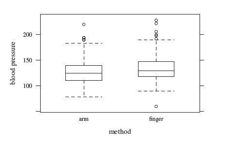
Figure 10.3 Side-by-side boxplots for unreplicated blood pressure data.
Table 10.1 Nonparametric and parametric estimates for measures of similarity and agreement for unreplicated blood pressure data. The parametric estimates are based on the bivariate normal model (4.6). Lower bounds for CCC and upper bounds for TDI are presented. Methods 1 and 2 refer to arm and finger methods, respectively.

They are consistent with what we expect from the exploratory analysis. They also lead to an estimated mean of 4.3 and standard deviation of 14.5 for the difference D = Y2 − Y1. The standard deviation is rather large mainly due to the modest correlation between the methods.
Table 10.1 presents plug-in estimates of the similarity measures µ2 − µ1 and σ22/σ21, and and the agreement measures CCC and TDI(0.90). Also presented are two-sided 95% intervals for the similarity measures and one-sided 95% bounds for the agreement measures. These use percentiles of a standard normal distribution as critical points because only two methods are compared. The critical points are 1.96 for the mean difference and log of variance ratio, 1.645 for the Fisher’s z-transformation of CCC, and −1.645 for the TDI bound, which is computed using (10.15). The interval for µ2 − µ1 ranges from 2.3 to 6.3, implying a larger mean for the finger method compared to the arm method. The interval for σ22/σ12 is barely to the right of one, providing borderline evidence for higher variability of the finger method. Thus, on the whole, the methods do not have similar characteristics.
The CCC lower bound of 0.75 suggests a weak agreement in the methods. The TDI upper bound of 28 also suggests this conclusion by clearly showing that the methods cannot be considered to have acceptable agreement because doing so would amount to treating a 28 mm Hg difference in blood pressure as clinically acceptable. It is also apparent from the similarity evaluation that no simple recalibration can bring the two methods into acceptable agreement. Although subtracting 4.3 from the finger’s measurements makes its mean match that of the arm’s, the resulting improvement in CCC and TDI bounds, now at 0.77 and 26.3, respectively, is not large enough for the conclusion to change. For further improvement, the correlation between the methods needs to increase, for example, by increasing the precisions of the methods, thereby reducing the size of the differences.
Even though the normality assumption does not hold for these data, it is of interest to analyze them anyway using a normality-based approach and compare conclusions. The relevant methodology is the one in Chapter 4 that assumes the bivariate normal model (4.6) for the data. Table 10.1 also presents the resulting parametric inferences. We see that the two estimates of every moment-based measure are identical. This is expected because the ML estimators of the first-and second-order moments under (4.6) are also the nonparametric plug-in estimators (Exercise 10.2). But even the confidence intervals and bounds for these measures are identical to the number of decimal places reported. In addition, although the two estimates and bounds for TDI are not identical, there is little practical difference between them. Overall, this seems to suggest that the skewness of these data is not severe enough to invalidate the parametric analysis. Note also that the number of subjects here (n = 200) is relatively large.
10.5.2 Replicated Blood Pressure Data
This dataset, introduced in Exercise 7.12, has three replicate measurements of systolic blood pressure (mm Hg) taken in quick succession on 85 subjects by each of two experienced observers named “J” (method 1) and “R” (method 2) using a sphygmomanometer, and by a semi-automatic blood pressure monitor (method 3). We treat these as unlinked repeated measurements data. The design is balanced with a total of 85 × 3 × 3 = 765 observations ranging from 74 to 228 mm Hg. We are interested in all-pairwise comparisons involving the three methods.
A trellis plot of the data is displayed in Figure 10.4. The measurements of the two observers largely overlap, but those of the monitor tend be larger than theirs. It also has a higher within-subject variation than the observers. This variation does not seem to depend on the measurement’s magnitude in a consistent manner. Also, as in the previous dataset, some subjects have large differences between monitor’s and observers’ measurements, suggesting skewness in the distributions of their differences. But none of the observations is a clear outlier. Figure 10.5 displays a matrix of scatterplots and the corresponding Bland-Altman plots for a subset of data consisting of one measurement per method selected randomly for every subject. The scatterplots show a very high correlation between the observers but only modest correlations between the observers and the monitor. The Bland-Altman plots do not have any trend, implying a common scale for the methods. These plots also corroborate the monitor’s tendency to produce larger measurements than the observers’. The side-by-side boxplots of all measurements from the three methods are displayed in Figure 10.6. Besides confirming the foregoing observation, they also show that the two observers have remarkably similar marginal distributions. In addition, there is clear right-skewness in all three marginal distributions, invalidating the normality assumption for the data (Exercise 7.12).
To get the empirical cdf ![]() , 33 = 27 triplets (or 3-tuples) are formed for each subject using the repeated measurements of the three methods. This results in a total of 85 × 27 = 2295 triplets in the data. Therefore, from (10.4),
, 33 = 27 triplets (or 3-tuples) are formed for each subject using the repeated measurements of the three methods. This results in a total of 85 × 27 = 2295 triplets in the data. Therefore, from (10.4), ![]() is a trivariate cdf that gives a weight of 1 /2295 to each triplet. From Exercise 10.15, the plug-in estimates of (mean, standard deviation) of measurements from methods 1, 2, and 3 are (127.4, 31.0), (127.3, 30.7), and (143.0, 32.5), respectively. In addition, the estimated correlation between the methods in the pairs (1, 2), (1, 3), and (2, 3) are 0.97, 0.79, and 0.79, respectively. Thus, the two observers have practically the same estimated means and variances, and their correlation is very high. On the other hand, the monitor produces higher readings than the observers by about 16 mm Hg on average and correlates less with their measurements. It also has a somewhat higher variability than the observers. The standard deviation of the difference between two observers is about 7 and it is three times as much for the difference between the monitor and an observer.
is a trivariate cdf that gives a weight of 1 /2295 to each triplet. From Exercise 10.15, the plug-in estimates of (mean, standard deviation) of measurements from methods 1, 2, and 3 are (127.4, 31.0), (127.3, 30.7), and (143.0, 32.5), respectively. In addition, the estimated correlation between the methods in the pairs (1, 2), (1, 3), and (2, 3) are 0.97, 0.79, and 0.79, respectively. Thus, the two observers have practically the same estimated means and variances, and their correlation is very high. On the other hand, the monitor produces higher readings than the observers by about 16 mm Hg on average and correlates less with their measurements. It also has a somewhat higher variability than the observers. The standard deviation of the difference between two observers is about 7 and it is three times as much for the difference between the monitor and an observer.
For similarity evaluation, Table 10.2 presents estimates and 95% simultaneous confidence intervals for the three all-pairwise mean differences and variance ratios. The critical point for the former is 2.24 and it is 2.25 for the latter on the log scale. The first interval for mean difference is tight around zero, implying no difference in the means of the two observers. The other two intervals are essentially identical and confirm that the monitor has a higher mean than the observers. The first interval for variance ratio, although barely covering one, is quite tight around 1.02. The value of 1 is deep inside the remaining two intervals, which are also essentially identical. This suggests that all methods can be taken to have the same variance. Overall, the two observers have very similar characteristics, but the same is not true for the monitor-observer pairs due to the larger mean of the monitor.
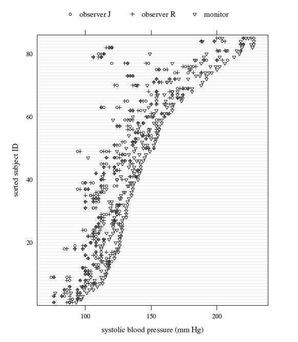
Figure 10.4 Trellis plot of replicated blood pressure data.
For agreement evaluation, Table 10.3 presents estimates and 95% simultaneous one-sided confidence bounds for the three all-pairwise CCCs and TDIs with p = 0.90. The critical point is 1.92 for CCC after applying the Fisher’s z-transformation. The TDI critical point, for use in (10.15), is 1.99. The TDI bounds imply that for 90% of subjects the measurement differences between method pairs (1, 2), (1, 3), and (2, 3) are estimated to lie between ±14, ±54, and ±53, respectively. The value of 14 is about 11% of the average value for the observers. This extent of agreement can be considered acceptable. However, this is clearly not the case for the two monitor-observer pairs that have quite similar extent of agreement. The same conclusion is reached on the basis of CCC bounds. It is also evident that the monitor’s unacceptable agreement with the observers is caused by a large mean difference and a relatively low correlation that itself is a consequence of the monitor’s relatively high within-subject variation (see the trellis plot in Figure 10.4). The first cause can be fixed by subtracting 15.6 from the monitor’s measurements. But this recalibration helps only to a limited extent as the new TDI bounds for (1, 3) and (2, 3) pairs are still high at 40 and 38, respectively, and both the new CCC bounds are still relatively low at 0.78. Further improvement requires reducing the monitor’s error variation, which cannot be achieved by a simple recalibration.
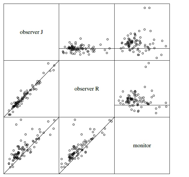
Figure 10.5 A matrix of scatterplots of systolic blood pressures with line of equality (below the diagonal) and Bland-Altman plots with zero line (above the diagonal) for replicated blood pressure data. One measurement per method from each of the 85 subjects is randomly selected for this plot. The measurements range from 76 to 227 mm Hg and their differences range from −25 to 111 mm Hg.
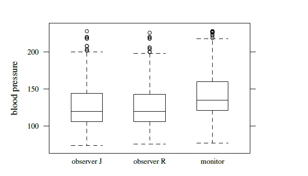
Figure 10.6 Side-by-side boxplots for all measurements of replicated blood pressure data.
Table 10.2 Estimates and two-sided 95% simultaneous confidence intervals for all-pairwise mean differences and variance ratios for replicated blood pressure data. Methods 1, 2, and 3 refer to observers J and R and the monitor, respectively.

Table 10.3 Estimates and one-sided 95% simultaneous confidence bounds for all-pairwise CCCs and TDIs (with p = 0.90) for replicated blood pressure data. Methods 1, 2, and 3 refer to observers J and R and the monitor, respectively.

For these data also, it may be of interest to compare these results with a normality-based parametric analysis even though the normality assumption does not hold here. However, the standard mixed-effects model (7.7) for unlinked repeated measurements data does not provide a reliable fit and an alternative model is fit in Exercise 7.12. Comparison of results under this model is left to Exercise 10.15.
10.6 CHAPTER SUMMARY
- The methodology presented here is a nonparametric analog of the normality-based approach developed in Chapters 4, 5 and 7 for J ( ≥ 2) methods for unreplicated and unlinked repeated measurements data.
- It makes no assumption about the shape of the data distribution.
- No assumption is needed about scales for the measurement methods. But the data are assumed to be homoscedastic.
- It allows for simultaneous inference on pairwise measures when more than two methods are compared.
- It takes a statistical functional approach where population quantities are considered features of the population distribution and are estimated using the same features of the empirical distribution.
- Weights are used to get the empirical distribution for repeated measurements data.
- The design for repeated measurements data may be balanced or unbalanced.
- For balanced designs and large number of subjects, the nonparametric inferences on moment-based measures are often similar to their normality-based counterparts.
- The observed measurements are not decomposed into true values and errors, precluding the use of similarity measures such as bias difference and precision ratio. Instead, mean difference and variance ratio are used.
- The methodology is valid for large number of subjects.
10.7 TECHNICAL DETAILS
Let Y be the support of the population vector Y =(Y1,...,YJ)T with cdf F(y) and pdf or pmf pF(y). Let S denote the index set of Q pairs of the form (j, l), j < l = 1, ..., J indicating the specific method pairs of interest. For a (j, l) ∈ S, a measure of similarity or agreement can be written as a statistical functional φjl = hjl(F), where hjl is a known real-valued function defined over a class F of J-variate cdfs on Y for which φjl is well-defined. The measures of interest in this chapter are represented as statistical functionals and these are defined in terms of expectations that are assumed to exist. An expectation can be explicitly written as a statistical functional in the following manner:
 (10.16)
where
Let ![]() denote the Q × 1 vector of values of a measure for the method pairs of interest. Its components are
denote the Q × 1 vector of values of a measure for the method pairs of interest. Its components are ![]() jl, (j, l) ∈S, and it is also a statistical functional
jl, (j, l) ∈S, and it is also a statistical functional ![]() = h(F), where the function h : F → RQ essentially stacks the hjl in a Q × 1 vector. The plug-in estimator of φ is
= h(F), where the function h : F → RQ essentially stacks the hjl in a Q × 1 vector. The plug-in estimator of φ is ![]() = h(
= h(![]() ), a Q × 1 vector with components
), a Q × 1 vector with components ![]() jl = hjl(
jl = hjl(![]() ). Under certain assumptions,
). Under certain assumptions, ![]() approximately follows a
approximately follows a ![]() distribution when n is large. Assuming that we know how to compute the Q × Q estimated covariance matrix
distribution when n is large. Assuming that we know how to compute the Q × Q estimated covariance matrix ![]() , this result can be used just as in Chapter 7 to obtain appropriate simultaneous confidence bounds and intervals for the Q values of a measure of interest.
, this result can be used just as in Chapter 7 to obtain appropriate simultaneous confidence bounds and intervals for the Q values of a measure of interest.
10.7.1 The Ω Matrix
To compute ![]() , we first need its population counterpart, the Q × Q covariance matrix Ω. It is defined in terms of variances and covariances of the influence function of the measure. The influence function of a scalar functional h(F) measures the rate at which the functional changes when F is contaminated by a small probability of contamination y. It plays a key role in the theory of nonparametric and robust estimators. To define it, let δy be the cdf of a J-variate distribution that assigns probability 1 to the point y. Then, the influence function of h(F) is
, we first need its population counterpart, the Q × Q covariance matrix Ω. It is defined in terms of variances and covariances of the influence function of the measure. The influence function of a scalar functional h(F) measures the rate at which the functional changes when F is contaminated by a small probability of contamination y. It plays a key role in the theory of nonparametric and robust estimators. To define it, let δy be the cdf of a J-variate distribution that assigns probability 1 to the point y. Then, the influence function of h(F) is
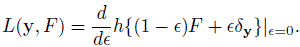 (10.17)
Here (1 − ε)F + εδy is the cdf of a contaminated distribution under which the random vector follows the distribution F with probability 1 − ε and the distribution δy with probability ε. Being a function of Y = y, the influence function is a random quantity. Its expectation is taken to be zero by definition. For example, consider the expectation functional EF {a(Y)} given by (10.16). Its influence function is (Exercise 10.9)
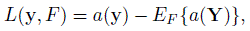 (10.18)
which obviously has expectation zero.
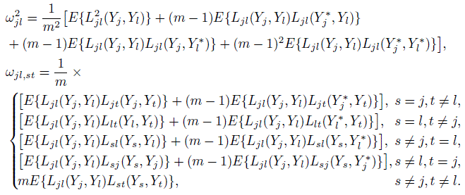
Let Ljl(yj, yl) ≡ Ljl(y, F ) denote the influence function of the measure φjl, (j, l) ∈ S. Next, let ω2jl and ωjl,st, (j, l) ≠ (s, t) ∈ S, respectively, denote the diagonal and the offdiagonal elements of Ω. Also let Yj∗ be a replication of Yj, j = 1,..., J from the same subject. The elements of Ω can be written in terms of the influence functions as:
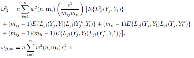
 (10.19)
The expectations here are with respect to the distribution F ; it has been dropped from the notation to reduce clutter. The expressions simplify when the design is balanced (Exercise 10.10). In particular, Ω does not depend on n anymore. Further simplification occurs for unreplicated measurements. Taking mij = 1 for all i, j in (10.19) yields
 (10.20)
Thus, in the unreplicated case, ω2jl is the variance of the influence function of φjl, and ωjl, st is the covariance between the influence functions of φjl and φst, regardless of whether the method pairs (j, l) and (s, t) contain any common methods. In addition, if J = 2, we have Q = 1, and the matrix Ω simply represents the scalar quantity ω212.
10.7.2 Estimation of Ω
Let ![]() the empirical counterpart of the influence function
the empirical counterpart of the influence function ![]() The estimator
The estimator ![]() of Ω can be obtained by replacing the population moments of Ljl(Yj, Yl) in (10.19) with their sample analogs based on
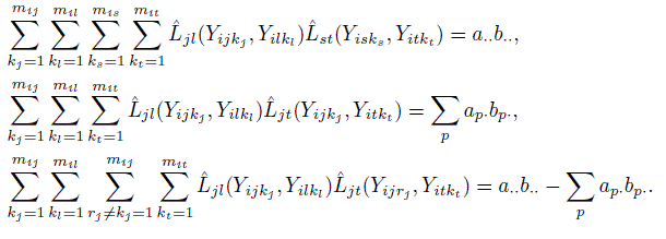
of Ω can be obtained by replacing the population moments of Ljl(Yj, Yl) in (10.19) with their sample analogs based on ![]() jl(Yj, Yl). Essentially the latter can be obtained by first computing the corresponding sample moments for each subject separately and then averaging them to come up with overall estimates. Specifically, the four moments needed for estimating ω2jl can be estimated in the following manner:
jl(Yj, Yl). Essentially the latter can be obtained by first computing the corresponding sample moments for each subject separately and then averaging them to come up with overall estimates. Specifically, the four moments needed for estimating ω2jl can be estimated in the following manner:

Next, consider the moments needed for ωjl,st. We can estimate the moment of the form E {Ljl(Yj, Yl) Lst(Ys, Yt)} by
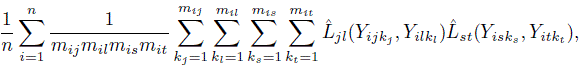
where if s = j (or s = l), mis is removed from the denominator and the sum over ks is restricted to ks = kj (or ks = kl); and a similar modification is made if t = j or t = l. Further, E {Ljl(Yj, Yl) Ljt(Y∗j, Yt)} can be estimated as

One can proceed in a similar manner to estimate the remaining three moments, namely, ![]() and
and ![]() See Exercises 10.11 and 10.12 for compact expressions for the inner multiple sums involved in these estimates.
See Exercises 10.11 and 10.12 for compact expressions for the inner multiple sums involved in these estimates.
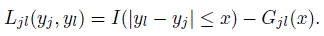
10.7.3 Influence Functions for the Measures
The influence functions Ljl(yj, yl) for the measures φjl of similarity and agreement considered in Section 10.4 are as follows (Exercise 10.13):
 (10.21)
where gjl is the pdf of | Yl − Yj | with cdf Gjl. The empirical counterparts of these influences are used as in Section 10.7.2 to estimate the covariance matrix for the estimated measures.
10.7.4 TDI Confidence Bounds
From the TDI’s influence function in (10.21), it is clear that an estimate of the pdf gjl at an estimated TDI—typically a relatively large percentile—is needed to compute SEs and confidence bounds. However, as mentioned previously, density estimates in the tails are generally not stable unless n is quite large. If one is willing to forgo the SEs, the density estimation can be avoided by using the confidence bounds (10.15). For this, one works with the cdf Gjl instead of its inverse. To be precise, φjl = Gjl(x) for an appropriate x is taken as the agreement measure. (Recall from Chapter 2 that this measure is in fact the index coverage probability defined by (2.24).) It is estimated as ![]() jl =
jl = ![]() jl(x). Being an expectation functional, its influence function from Exercise 10.9 is
jl(x). Being an expectation functional, its influence function from Exercise 10.9 is
 (10.22)
With ![]() as x, one proceeds in the same way as for other measures to compute simultaneous upper confidence bounds for φjl, (j, l) ∈ S. These have the form
as x, one proceeds in the same way as for other measures to compute simultaneous upper confidence bounds for φjl, (j, l) ∈ S. These have the form
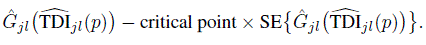
Thereupon, the estimate ![]() in the first term in the expression above is replaced by p, the quantity it actually estimates, and G−1jl is evaluated at the resulting value, yielding the bounds given in (10.15).
in the first term in the expression above is replaced by p, the quantity it actually estimates, and G−1jl is evaluated at the resulting value, yielding the bounds given in (10.15).
10.7.5 Summary of Steps
To summarize, the steps involved in constructing nonparametric simultaneous confidence intervals for φjl, (j, l) ∈ S are as follows:
- Estimate the cdf F by the empirical cdf
 using (10.2).
 - Compute the plug-in estimate
 jl = hjl() using the joint pmf (10.7) of (Yj , Yl) under .
 - Compute the empirical influences
 jl(Yj, Yl) for each observed pair (Yijkj, Yilkl), kj = 1,...,mij, kl = 1,...,mil using (10.21) or (10.22).
 - Repeat steps 2 and 3 for each (j, l) ∈ S to get the estimate of the vector
 and compute its estimated covariance matrix n−1
 .
. - Apply the methodology of Section 3.3 to compute appropriate critical points for simultaneous bounds and intervals and use them in (10.14) and (10.15).
10.8 BIBLIOGRAPHIC NOTE
The nonparametric methodology of this chapter is largely based on Choudhary (2010). The article provides the underlying technical details, including a derivation of the asymptotic normality of plug-in estimators under a specified set of assumptions. The use of weights to compute empirical cdf from repeated measurements data is motivated by Olsson and Rootzén (1996), who focus on nonparametric estimation of quantiles of a single variable. Both articles also present a comparison of estimators obtained using different weight functions in the case of unbalanced designs. Lehmann (1998) provides a gentle introduction to nonparametric estimation, statistical functionals, and influence functions. More rigorous and complete accounts are given by Fernholz (1983) and van der Vaart (1998).
A key attraction of the statistical functional approach is that it provides a unified nonparametric framework for inference on various measures of similarity and agreement. In the method comparison literature, it was first used by Guo and Manatunga (2007), although only for inference on CCC with unreplicated data under univariate censoring. For CCC, an alternative approach based on U-statistics has been developed by King and Chinchilli and their coauthors in a number of articles, including King and Chinchilli (2001a, b) and King et al. (2007a, b). The two nonparametric approaches for CCC differ in assumptions, but are expected to lead to similar inferences when n is large. For TDI, an alternative approach based on order statistics is proposed in Perez-Jaume and Carrasco (2015). This article also compares the two nonparametric approaches for TDI.
The normality-based methodologies may lead to inaccurate inferences for non-normal method comparison data. This has been demonstrated by Carrasco et al. (2007) for CCC and by Perez-Jaume and Carrasco (2015) for TDI. We have illustrated a nonparametric approach for handling non-normal data. An alternative is to use a parametric mixed-effects model approach based on distributions other than the normal, for example, a lognormal distribution for random effects (Carrasco et al., 2007), or more general skewed and heavy-tailed distributions for random effects or errors that include the normal as a special case (Sengupta et al., 2015). These model-based approaches work for both CCC and TDI. Yet another alternative, though only for moment-based measures such as CCC, is to use GEE to directly model the moments rather than modeling the entire data distribution. Such a semiparametric approach has been taken by a number of authors, including Barnhart and Williamson (2001), Barnhart et al. (2002, 2005), and Lin et al. (2007). The moment-based measures may be unduly affected by outliers in the data. King and Chinchilli (2001b) address this issue for CCC in the case of paired measurements data by developing its robust versions. Their approach is to replace the squared-error distance function built into the definition of CCC by alternate functions that are less susceptible to outliers, for example, absolute error distance functions and their Winsorized versions. A similar approach can be adopted for the other measures.
Data Sources
The unreplicated and the replicated blood pressure data are from Bland and Altman (1995b) and Bland and Altman (1999), respectively. They can be obtained from the book’s website.
EXERCISES
- Suppose a scalar random variable X follows a probability distribution with cdf G(x). Let g(x) denote the pdf if X is continuous and the pmf if it is discrete. Define the notation,
where X is the support of x. Also, define the inverse cdf G(x) as G−1 (u) = min{x : G(x) ≥ u}.
- Write the mean and variance of X as statistical functionals.
- Write the 100pth percentile of X as a statistical functional.
- Consider the empirical cdf given by (10.1) for estimating F from unreplicated data. There may be ties among observations from a given method.
Show that the joint pmf of (Y1,...,YJ) under
is
Show that the joint pmf of (Yj, Yl) under
is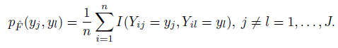
Show that the marginal pmf of Yj under
is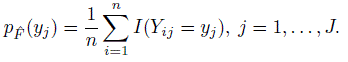
- Let h(F) be the population mean of Yj. Show that the plug-in estimator h() is the sample mean
 ·j.
·j. - Let h(F) be the population variance of Yj. Show that the plug-in estimator h() is the sample variance
 with divisor n.
 - Let h(F) be the population covariance between Yj and Yl. Show that the plugin estimator is the sample covariance
 with divisor n.
 - Let h(F) be the population correlation between Yj and Yl. Show that the plug-in estimator h() is the sample correlation between Yj and Yl.
- Let h(F) be the 100pth population percentile of Yj. Show that the plug-in estimator
 where j is the cdf associated with the pmf given in part (c).
 - Show that the plug-in estimators of means, variances, and correlation of Yj and Yl obtained in previous parts are identical to the ones in (10.10). (When J = 2, they are also identical to the ML estimators given by (4.8) under the bivariate normal model (4.6).)
- Verify the expressions for the pmfs given in (10.6)–(10.8) under the empirical distribution (10.2) for (Y1,...,YJ).
- (Continuation of Exercise 10.3) Assume now that there are no within-method ties in the data. Establish the following:
- (Continuation of Exercise 10.4) Assume further that the design is balanced with all mij = m. Show that the pmfs in Exercise 10.4 simplify to the following expressions:

for kj = 1,...,m, j ≠ l = 1,..., J, i = 1,...,n.
- Consider the cdf defined in (10.2) with weight function w satisfying the unbiasedness condition (10.3). Assume that the indicator functions I involved in have a common correlation ρ(y), with y =(y1,...,yJ)T.
Show that the optimal weight function that makes
(y) the minimum variance unbiased estimator of F(y) in the family of estimators satisfying (10.2) and (10.3) is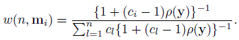
- The optimal weight function depends on y through ρ(y). Discuss its impact on the properties of . In particular, does it guarantee (y) to be non-decreasing in y—a property necessary for to be a valid cdf?
- For a balanced design, show that the optimal function reduces to (10.4).
- For an unbalanced design, show that the optimal function reduces to w1 and w2 given in (10.5) when ρ(y) = 1 and ρ(y)= 0, respectively.
(This exercise offers a straightforward generalization of a similar result in Olsson and Rootzén (1996) for univariate distribution.)
- Show that the measures of similarity and agreement considered in Section 10.4 can be written as statistical functionals in the following manner:
where

- (a) Show that the estimated cdf in (10.11) can be written as

Show that the estimated moments in (10.9) can be written as

- Consider the expectation functional EF {a(Y)} given by (10.16). Show that its influence function is L(y, F) = a(y) − EF {a(Y)}.
- When the design is balanced with all mij = m, show that the elements of Ω given in (10.19) have the following simplified expressions:
- Let A denote an mij × mil matrix with (p, q)th element apq = jl(Yijp, Yilq). Define the column sum
 the row sum
  and the overall sum
 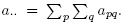 Also define the sums of squares:
 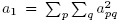 ,
,  and a4 = a..2. Verify the following compact expressions for the multiple sums involved in estimation of ω2jl in Section 10.7.2:
- (Continuation of Exercise 10.11) Let B denote an mis × mit matrix with (u, v)th element
 Define the column sum
  the row sum
  and the overall sum
  . Verify the following expressions for the multiple sums involved in estimation of ωjl,st in Section 10.7.2:
- Use the definition (10.17) of an influence function to verify the forms for influence functions given in (10.21) for the measures of similarity and agreement considered. [Hint: For the first three, use Exercise 10.9 and apply the chain rule if needed. For the last, use implicit differentiation.]
- Consider the unreplicated blood pressure data from Section 10.5.1.
- Perform model diagnostics to verify that the bivariate normal model (4.6) does not fit these data well.
- Verify the results of the nonparametric and parametric analyses in Table 10.1.
- (Continuation of Exercise 7.12) Consider the replicated blood pressure data from Exercise 7.12 and Section 10.5.2.
- Determine the nonparametric estimates of means, variances, and correlations for the three methods.
- Determine the nonparametric estimates of means and standard deviations of Dij, j = 1, 2, 3.
- Verify the results of the nonparametric analysis in Tables 10.2 and 10.3.
- Compare conclusions with those of the parametric analysis carried out in Exercise 7.12.
- Which analysis, nonparametric or parametric, would you recommend? Why?
- Table 10.4 presents lengths (in mm) of 25 fiddler crab claws measured by an observer using two Mitutoyo vernier calipers. There are three unlinked replications of each measurement. These data are a subset of the data analyzed in Choudhary et al. (2014) and focus only on observer 1.
- Perform an exploratory analysis of the data.
Table 10.4 Crab claws data consisting of lengths of crab claws (in mm) for Exercise 10.16. They are provided by P. Cassey.
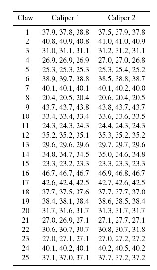
- Fit model (7.7) and perform model diagnostics. Does the normality assumption for residuals appear reasonable? Proceed with the normality-based parametric analysis regardless of your finding.
- Analyze the data using an appropriate nonparametric approach.
- Compare conclusions of the parametric and nonparametric analyses. Which analysis would you prefer? Why?