
CHAPTER ONE
Matrix Two-Person Games
If you must play, decide upon three things at the start: the rules of the game, the stakes, and the quitting time.
—Chinese proverb
Everyone has a plan until you get hit.
—Mike Tyson, Heavyweight Boxing Champ, 1986–1990, 1996
You can’t always get what you want.
—Mothers everywhere
1.1 The Basics
What is a game? We need a mathematical description, but we will not get too technical. A game involves a number of players1 N, a set of strategies for each player, and a payoff that quantitatively describes the outcome of each play of the game in terms of the amount that each player wins or loses. A strategy for each player can be very complicated because it is a plan, determined at the start of the game, that describes what a player will do in every possible situation. In some games, this is not too bad because the number of moves is small, but in other games, like chess, the number of moves is huge and so the number of possible strategies, although finite, is gigantic. In this chapter, we consider two-person games and give several examples of exactly what is a strategy.
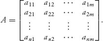
Let’s call the two players I and II. Suppose that player I has a choice of n possible strategies and player II has a choice of m possible strategies. If player I chooses a strategy, say, strategy i, i = 1, ..., n, and player II chooses a strategy j, j = 1, ..., m, then they play the game and the payoff to each player is computed. In a zero sum game, whatever one player wins the other loses, so if aij is the amount player I receives, then II gets −aij. Now we have a collection of numbers {aij}, i = 1, ..., n, j = 1, ..., m, and we can arrange these in a matrix. These numbers are called the payoffs to player I and the matrix is called the payoff or game matrix:
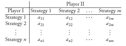
By agreement we place player I as the row player and player II as the column player. We also agree that the numbers in the matrix represent the payoff to player I. In a zero sum game, the payoffs to player II would be the negative of those in the matrix so we don’t have to record both of those. Of course, if player I has some payoff that is negative, then player II would have a positive payoff.
Summarizing, a two-person zero sum game in matrix form means that there is a matrix A = (aij), i = 1, ..., n, j = 1, ..., m of real numbers so that if player I, the row player, chooses to play row i and player II, the column player, chooses to play column j, then the payoff to player I is aij and the payoff to player II is −aij. Both players want to choose strategies that will maximize their individual payoffs. Player I wants to choose a strategy to maximize the payoff in the matrix, while player II wants to choose a strategy to minimize the corresponding payoff in the matrix. That is because the game is zero sum.
Remark Constant Sum Matrix Games. The discussion has assumed that whatever one player wins the other player loses, that is, that it is zero sum. A slightly larger class of games, the class of constant sum games, can also be reduced to this case. This means that if the payoff to player I is aij when player I uses row i and II uses column j, then the payoff to player II is C − aij, where C is a fixed constant, the same for all rows and columns. In a zero sum game, C = 0. Now note that even though this is nonzero sum, player II still gets C minus whatever player I gets. This means that from a game theory perspective, the optimal strategies for each player will not change even if we think of the game as zero sum. If we solve it as if the game were zero sum to get the optimal result for player I, then the optimal result for player II would be simply C minus the optimal result for I.
Now let’s be concrete and work out some examples.
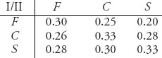
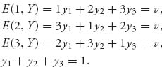
Example 1.1 Pitching in Baseball. A pitcher has a collection of pitches that he has developed over the years. He can throw a fastball (F), curve (C), or slider (S). The batter he faces has also learned to expect one of these three pitches and to prepare for it. Let’s call the batter player I and the pitcher player II. The strategies for each player in this case are simple; the batter looks for F, C, or S, and the pitcher will decide to use F, C, or S. Here is a possible payoff, or game matrix, 2 to the batter:
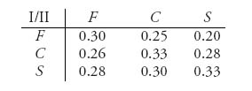
For example, if the batter, player I, looks for a fastball and the pitcher actually pitches a fastball, then player I has probability 0.30 of getting a hit. This is a constant sum game because player II’s payoff and player I’s payoff actually add up to 1. The question for the batter is what pitch to expect and the question for the pitcher is what pitch to throw on each play.
Example 1.2 Suppose that two companies are both thinking about introducing competing products into the marketplace. They choose the time to introduce the product, and their choices are 1 month, 2 months, or 3 months. The payoffs correspond to market share:
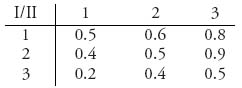
For instance, if player I introduces the product in 3 months and player II introduces it in 2 months, then it will turn out that player I will get 40% of the market. The companies want to introduce the product in order to maximize their market share. This is also a constant sum game.
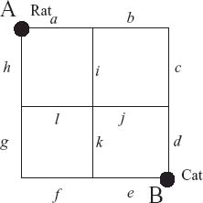
Example 1.3 Suppose an evader (called Rat) is forced to run a maze entering at point A. A pursuer (called Cat) will also enter the maze at point B. Rat and Cat will run exactly four segments of the maze and the game ends. If Cat and Rat ever meet at an intersection point of segments at the same time, Cat wins +1 (Rat) and the Rat loses −1 because it is zero sum, while if they never meet during the run, both Cat and the Rat win 0. In other words, if Cat finds Rat, Cat gets +1 and otherwise, Cat gets 0. We are looking at the payoffs from Cat’s point of view, who wants to maximize the payoffs, while Rat wants to minimize them. Figure 1.1 shows the setup.
The strategies for Rat consist of all the choices of paths with four segments that Rat can run. Similarly, the strategies for Cat will be the possible paths it can take. With four segments it will turn out to be a 16 × 16 matrix. It would look like this:
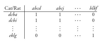
FIGURE 1.1 Maze for Cat versus Rat.
The strategies in the preceding examples were fairly simple. The next example gives us a look at the fact that they can also be complicated, even in a simple game.
Example 1.4 2 × 2 Nim. Four pennies are set out in two piles of two pennies each. Player I chooses a pile and then decides to remove one or two pennies from the pile chosen. Then player II chooses a pile with at least one penny and decides how many pennies to remove. Then player I starts the second round with the same rules. When both piles have no pennies, the game ends and the loser is the player who removed the last penny. The loser pays the winner one dollar.
Strategies for this game for each player must specify what each player will do depending on how many piles are left and how many pennies there are in each pile, at each stage. Let’s draw a diagram of all the possibilities (see Figure 1.2).
FIGURE 1.2 2 × 2 Nim tree.
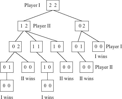
When the game is drawn as a tree representing the successive moves of a player, it is called a game in extensive form.
Next, we need to write down the strategies for each player:
| Strategies for player I |
| (1) Play (1, 2) then, if at (0, 2) play (0, 1). |
| (2) Play (1, 2) then, if at (0, 2) play (0, 0). |
| (3) Play (0, 2). |
You can see that a strategy for I must specify what to do no matter what happens. Strategies for II are even more involved:
| Strategies for player II |
| (1) If at (1, 2) → (0, 2); if at (0, 2) → (0, 1) |
| (2) If at (1, 2)→ (1, 1); if at (0, 2)→ (0, 1) |
| (3) If at (1, 2)→ (1, 0); if at (0, 2)→ (0, 1) |
| (4) If at (1, 2)→ (0, 2); if at (0, 2)→ (0, 0) |
| (5) If at (1, 2)→ (1, 1); if at (0, 2)→ (0, 0) |
| (6) If at (1, 2)→ (1, 0); if at (0, 2)→ (0, 0) |
Playing strategies for player I against player II results in the payoff matrix for the game, with the entries representing the payoffs to player I.
Analysis of 2 × 2 Nim. Looking at this matrix, we see that player II would never play strategy 5 because player I then wins no matter which row I plays (the payoff is always +1). Any rational player in II’s position would drop column 5 from consideration (column 5 is called a dominated strategy). By the same token, if you look at column 3, this game is finished. Why? Because no matter what player I does, player II by playing column 3 wins +1. Player I always loses as long as player II plays column 3; that is, if player I goes to (1, 2), then player II should go to (1, 0). If player I goes to (0, 2), then player II should go to (0, 1). This means that II can always win the game as long as I plays first.
We may also look at this matrix from I’s perspective, but that is more difficult because there are times when player I wins and times when player I loses when I plays any fixed row. There is no row that player I can play in which the payoff is always the same and so, in contrast to the column player, no obvious strategy that player I should play.
We say that the value of this game is −1 and the strategies
![]()
are saddle points, or optimal strategies for the players. We will be more precise about what it means to be optimal shortly, but for this example it means that player I can improve the payoff if player II deviates from column 3. Note that there are three saddle points in this example, so saddles are not necessarily unique.
This game is not very interesting because there is always a winning strategy for player II and it is pretty clear what it is. Why would player I ever want to play this game? There are actually many games like this (tic-tac-toe is an obvious example) that are not very interesting because their outcome (the winner and the payoff) is determined as long as the players play optimally. Chess is not so obvious an example because the number of strategies is so vast that the game cannot, or has not, been analyzed in this way.
One of the main points in this example is the complexity of the strategies. In a game even as simple as tic-tac-toe, the number of strategies is fairly large, and in a game like chess, you can forget about writing them all down.
The previous example is called a combinatorial game because both players know every move, and there is no element of chance involved. A separate branch of game theory considers only combinatorial games but this takes us too far afield and the theory of these games is not considered in this book.3
Here is one more example of a game in which we find the matrix by setting up a game tree. Technically, that means that we start with the game in extensive form.
Example 1.5 In a version of the game of Russian roulette, made infamous in the movie The Deer Hunter, two players are faced with a six-shot pistol loaded with one bullet. The players ante $1000, and player I goes first. At each play of the game, a player has the option of putting an additional $1000 into the pot and passing, or not adding to the pot, spinning the chamber and firing (at her own head). If player I chooses the option of spinning and survives, then she passes the gun to player II, who has the same two options. Player II decides what to do, carries it out, and the game ends.
The payoffs are now determined. If player I does not survive the first round shot, the game is over and II gets the pot. If player I has chosen to fire and survives, she passes the gun to player II; if player II chooses to fire and survives, the game is over and both players split the pot. If I fires and survives and then II passes, both will split the pot. The effect of this is that II will pay I $500. On the other hand, if I chooses to pass and II chooses to fire, then, if II survives, he takes the pot.
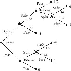
Remember that if either player passes, then that player will have to put an additional $1000 in the pot. We begin by drawing in Figure 1.3 (below) the game tree, which is nothing more than a picture of what happens at each stage of the game where a decision has to be made.
The numbers at the end of the branches are the payoffs to player I. The number ![]() , for example, means that the net gain to player I is $500 because player II had to pay $1000 for the ability to pass and they split the pot in this case. The circled nodes are spots at which the next node is decided by chance. You could even consider Nature as another player.
, for example, means that the net gain to player I is $500 because player II had to pay $1000 for the ability to pass and they split the pot in this case. The circled nodes are spots at which the next node is decided by chance. You could even consider Nature as another player.
The next step is to determine the (pure) strategies for each player.
For player I, this is easy because she makes only one choice at the start of the game and that is spin (I1) or pass (I2).
Player II also has one decision to make but it depends on what player I has done and the outcome of that decision. That’s why it’s called a sequential game. The pure strategies for player II are summarized in the following table.
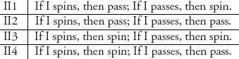
In each of these strategies, it is assumed that if player I spins and survives the shot, then player II makes a choice. Of course if player I does not survive, then player II walks away with the pot.
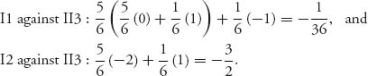
The payoffs are now random variables and we need to calculate the expected payoff 4 to player I. In I1 against II1, the payoff to I is ![]() with probability
with probability ![]() and −1 with probability
and −1 with probability ![]() . The expected payoff to I is then
. The expected payoff to I is then
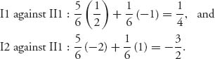
Strategy II3 says the following: If I spins and survives, then spin, but if I passes, then spin and fire. The expected payoff to I is
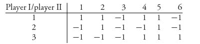
Continuing in this way, we play each pure strategy for player I against each pure strategy for player II. The result is the following game matrix:
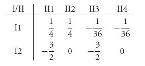
Now that we have the game matrix we may determine optimal strategies. This game is actually easy to analyze because we see that player II will never play II1, II2, or II4 because there is always a strategy for player II in which II can do better. This is strategy II3 that gives player II ![]() if I plays I1, or
if I plays I1, or ![]() if I plays I2. But player I would never play I2 if player II plays II3 because
if I plays I2. But player I would never play I2 if player II plays II3 because ![]() The optimal strategies then for each player are I1 for player I, and II3 for player II. Player I should always spin and fire. Player II should always spin and fire if I has survived his shot. The expected payoff to player I is −
The optimal strategies then for each player are I1 for player I, and II3 for player II. Player I should always spin and fire. Player II should always spin and fire if I has survived his shot. The expected payoff to player I is −![]()
The dotted line in Figure 1.3 indicates the optimal strategies. The key to these strategies is that no significant value is placed on surviving.
FIGURE 1.3 Russian roulette.
Remark Even though the players do not move simultaneously, they choose their strategies simultaneously at the start of the game. That is why a strategy needs to tell each player what to do at each stage of the game. That’s why they can be very complicated.
Remark Drawing a game tree is called putting the game into extensive form. Extensive form games can take into account sequential moves as well as the information available to each player when they have to make a choice. We will study extensive form games in more detail in a later chapter.
Remark The term pure referring to a strategy is to used to contrast what is to come when we refer to mixed strategies. Pure strategies are rows (or columns) that may be played. Mixed strategies allow a player to mix up the rows. Our next example introduces this concept.
In our last example, it is clear that randomization of strategies must be included as an essential element of games.
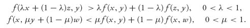
Example 1.6 Evens or Odds. In this game, each player decides to show one, two, or three fingers. If the total number of fingers shown is even, player I wins +1 and player II loses −1. If the total number of fingers is odd, player I loses −1 and player II wins +1. The strategies in this game are simple: deciding how many fingers to show. We may represent the payoff matrix as follows:
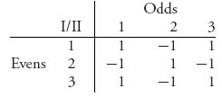
The row player here and throughout this book will always want to maximize his payoff, while the column player wants to minimize the payoff to the row player, so that her own payoff is maximized (because it is a zero or constant sum game). The rows are called the pure strategies for player I, and the columns are called the pure strategies for player II.
The following question arises: How should each player decide what number of fingers to show? If the row player always chooses the same row, say, one finger, then player II can always win by showing two fingers. No one would be stupid enough to play like that. So what do we do? In contrast to 2 × 2 Nim or Russian roulette, there is no obvious strategy that will always guarantee a win for either player.
Even in this simple game we have discovered a problem. If a player always plays the same strategy, the opposing player can win the game. It seems that the only alternative is for the players to mix up their strategies and play some rows and columns sometimes and other rows and columns at other times. Another way to put it is that the only way an opponent can be prevented from learning about your strategy is if you yourself do not know exactly what pure strategy you will use. That only can happen if you choose a strategy randomly. Determining exactly what this means will be studied shortly.
In order to determine what the players should do in any zero sum matrix game, we begin with figuring out a way of seeing if there is an obvious solution. The first step is to come up with a method so that if we have the matrix in front of us we have a systematic and mathematical way of finding a solution in pure strategies, if there is one.
We look at a game with matrix A = (aij) from player I’s viewpoint. Player I assumes that player II is playing her best, so II chooses a column j so as to
![]()
for any given row i. Then player I can guarantee that he can choose the row i that will maximize this. So player I can guarantee that in the worst possible situation he can get at least
![]()
and we call this number v− the lower value of the game. It is also called player I’s game floor.
Next, consider the game from II’s perspective. Player II assumes that player I is playing his best, so that I will choose a row so as to
![]()
for any given column j = 1, ..., m. Player II can, therefore, choose her column j so as to guarantee a loss of no more than
![]()
and we call this number v+ the upper value of the game. It is also called player II’s loss ceiling.
In summary, v− represents the least amount that player I can be guaranteed to receive and v+ represents the largest amount that player II can guarantee can be lost. This description makes it clear that we should always have v− ≤ v+ and this will be verified in general later.
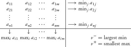
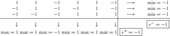
Here is how to find the upper and lower values for any given matrix. In a two-person zero sum game with a finite number of strategies for each player, we write the game matrix as
For each row, find the minimum payoff in each column and write it in a new additional last column. Then the lower value is the largest number in that last column, that is, the maximum over rows of the minimum over columns. Similarly, in each column find the maximum of the payoffs (written in the last row). The upper value is the smallest of those numbers in the last row:
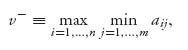
Here is the precise definition.
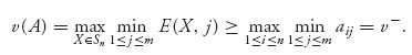
Definition 1.1.1 A matrix game with matrix An×m = (aij) has the lower value
and the upper value
![]()
The lower value v− is the smallest amount that player I is guaranteed to receive (v− is player I’s gain floor), and the upper value v+ is the guaranteed greatest amount that player II can lose (v+ is player II’s loss ceiling). The game has a value if v− = v+, and we write it as v = v(A)=v+ = v−. This means that the smallest max and the largest min must be equal and the row and column i*, j* giving the payoffs ai*, j* = v+ = v− are optimal, or a saddle point in pure strategies.
One way to look at the value of a game is as a handicap. This means that if the value v is positive, player I should pay player II the amount v in order to make it a fair game, with v = 0. If v < 0, then player II should pay player I the amount −v in order to even things out for player I before the game begins.
Example 1.7 Let’s work this out using 2 × 2 Nim.
We see that v− = largest min = −1 and v+ = smallest max = −1. This says that v+ = v− = −1, and so 2 × 2 Nim has v = −1. The optimal strategies are located as the (row, column) where the smallest max is −1 and the largest min is also −1. This occurs at any row for player I, but player II must play column 3, so i* = 1, 2, 3, j* = 3. The optimal strategies are not at any row column combination giving −1 as the payoff. For instance, if II plays column 1, then II will play row 1 and receive +1. Column 1 is not part of an optimal strategy.
We have mentioned that the most that I can be guaranteed to win should be less than (or equal to) the most that II can be guaranteed to lose (i.e., v− ≤ v+). Here is a quick verification of this fact.
Claim: v− ≤ v+. For any column j we know that for any fixed row i, minj aij ≤ aij, and so taking the max of both sides over rows, we obtain
![]()
This is true for any column j = 1, ..., m. The left side is just a number (i.e., v−) independent of i as well as j, and it is smaller than the right side for any j. However, this means that v− ≤ minj maxi aij = v+, and we are done.
Now here is a precise definition of a (pure) saddle point involving only the payoffs, which basically tells the players what to do in order to obtain the value of the game when v+ = v−.
Definition 1.1.2 We call a particular row i* and column j* a saddle point in pure strategies of the game if
(1.1)![]()
In words, (i*, j*) is a saddle point if when player I deviates from row i*, but II still plays j*, then player I will get less. Also, if player II deviates from column j* but I sticks with i*, then player I will do better. You can spot a saddle point in a matrix (if there is one) as the entry which is simultaneously the smallest in a row and largest in the column. A matrix may have none, one, or more than one saddle point. Here is a condition that guarantees at least one saddle.
Lemma 1.1.3 A game will have a saddle point in pure strategies if and only if
(1.2)![]()
Proof. If (1.1) is true, then
![]()
But v− ≤ v+ always, and so we have equality throughout and ![]()
On the other hand, if v+ = v− then
![]()
Let j* be such that v+ = maxi aij* and i* such that v− = minj ai*j. Then
![]()
In addition, taking j = j* on the left, and i = i* on the right, gives ![]() This satisfies the condition for (i*, j*) to be a saddle point.
This satisfies the condition for (i*, j*) to be a saddle point. ![]()
When a saddle point exists in pure strategies, Equation (1.1) says that if any player deviates from playing her part of the saddle, then the other player can take advantage and improve his payoff. In this sense, each part of a saddle is a best response to the other. This will lead us a little later into considering a best response strategy. The question is that if we are given a strategy for a player, optimal or not, what is the best response on the part of the other player?
We now know that v+ ≥ v− is always true. We also know how to play if v+ = v−. The issue is what do we do if v+ > v−. Consider the following example.
Example 1.8 In the baseball example player I, the batter expects the pitcher (player II) to throw a fastball, a slider, or a curveball. This is the game matrix:
A quick calculation shows that v− = 0.28 and v+ = 0.30. So baseball does not have a saddle point in pure strategies. That shouldn’t be a surprise because if there were such a saddle, baseball would be a very dull game, which nonfans say is true anyway. We will come back to this example below.
Problems
1.1 There are 100 bankers lined up in each of 100 rows. Pick the richest banker in each row. Javier is the poorest of those. Pick the poorest banker in each column. Raoul is the richest of those. Who is richer: Javier or Raoul?
1.2 In a Nim game start with 4 pennies. Each player may take 1 or 2 pennies from the pile. Suppose player I moves first. The game ends when there are no pennies left and the player who took the last penny pays 1 to the other player.
1.3 In the game rock-paper-scissors both players select one of these objects simultaneously. The rules are as follows: paper beats rock, rock beats scissors, and scissors beats paper. The losing player pays the winner $1 after each choice of object. If both choose the same object the payoff is 0.
1.4 Each of two players must choose a number between 1 and 5. If a player’s choice = opposing player’s choice +1, she loses $2; if a player’s choice ≥ opposing player’s choice +2, she wins $1. If both players choose the same number the game is a draw.
1.5 Each player displays either one or two fingers and simultaneously guesses how many fingers the opposing player will show. If both players guess either correctly or incorrectly, the game is a draw. If only one guesses correctly, he wins an amount equal to the total number of fingers shown by both players. Each pure strategy has two components: the number of fingers to show, the number of fingers to guess. Find the game matrix, v+, v−, and optimal pure strategies if they exist.
1.6 In the Russian roulette Example 1.5 suppose that if player I spins and survives and player II decides to pass, then the net gain to I is $1000 and so I gets all of the additional money that II had to put into the pot in order to pass. Draw the game tree and find the game matrix. What are the upper and lower values? Find the saddle point in pure strategies.
1.7 Let x be an unknown number and consider the matrices
![]()
Show that no matter what x is, each matrix has a pure saddle point.
1.8 If we have a game with matrix A and we modify the game by adding a constant C to every element of A, call the new matrix A + C, is it true that v+(A + C) = v+(A) + C?
1.9 Consider the square game matrix A = (aij) where aij = i − j with i = 1, 2, ..., n, and j = 1, 2, ..., n. Show that A has a saddle point in pure strategies. Find them and find v(A).
1.10 Player I chooses 1, 2, or 3 and player II guesses which number I has chosen. The payoff to I is |I's number − II's guess|. Find the game matrix. Find v− and v+.
1.11 In the Cat versus Rat game, determine v+ and v− without actually writing out the matrix. It is a 16 × 16 matrix.
1.12 In a football game, the offense has two strategies: run or pass. The defense also has two strategies: defend against the run, or defend against the pass. A possible game matrix is
![]()
This is the game matrix with the offense as the row player I. The numbers represent the number of yards gained on each play. The first row is run, the second is pass. The first column is defend the run and the second column is defend the pass. Assuming that x > 0, find the value of x so that this game has a saddle point in pure strategies.
1.13 Suppose A is a 2 × 3 matrix and A has a saddle point in pure strategies. Show that it must be true that either one column dominates another, or one row dominates the other, or both. Then find a matrix A which is 3 × 3 and has a saddle point in pure strategies, but no row dominates another and no column dominates another.
1.2 The von Neumann Minimax Theorem
Here now is the problem. What do we do when v− < v+? If optimal pure strategies don’t exist, then how do we play the game? If we use our own experience playing games, we know that it is rarely optimal and almost never interesting to always play the same moves. We know that if a poker player always bluffs when holding a weak hand, the power of bluffing disappears. We know that we have to bluff sometimes and hold a strong hand at others. If a pitcher always throws fastballs, it becomes much easier for a batter to get a hit. We know that no pitcher would do that (at least in the majors). We have to mix up the choices. John von Neumann figured out how to model mixing strategies in a game mathematically and then proved that if we allow mixed strategies in a matrix game, it will always have a value and optimal strategies. The rigorous verification of these statements is not elementary mathematics, but the theorem itself shows us how to make precise the concept of mixing pure strategies. You can skip all the proofs and try to understand the hypotheses of von Neumann’s theorem. The assumptions of the von Neumann theorem will show us how to solve general matrix games.
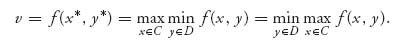
We start by considering general functions of two variables f = f(x, y), and give the definition of a saddle point for an arbitrary function f.
Definition 1.2.1 Let C and D be sets. A function ![]() has at least one saddle point (x*, y*) with x*
has at least one saddle point (x*, y*) with x* ![]() C and y*
C and y* ![]() D if
D if
![]()
Once again we could define the upper and lower values for the game defined using the function f, called a continuous game, by
![]()
You can check as before that v− ≤ v+. If it turns out that v+ = v− we say, as usual, that the game has a value v = v+ = v−. The next theorem, the most important in game theory and extremely useful in many branches of mathematics is called the von Neumann minimax theorem. It gives conditions on f, C, and D so that the associated game has a value v = v+=v−. It will be used to determine what we need to do in matrix games in order to get a value.
In order to state the theorem we need to introduce some definitions.
Definition 1.2.2 A set C ![]()
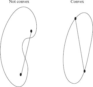
![]() n is convex if for any two points a, b
n is convex if for any two points a, b ![]() C and all scalars λ
C and all scalars λ ![]() [0, 1], the line segment connecting a and b is also in C, that is for all a, b
[0, 1], the line segment connecting a and b is also in C, that is for all a, b ![]() C, λ a + (1 − λ) b
C, λ a + (1 − λ) b ![]() C,
C, ![]() 0 ≤ λ ≤ 1.
0 ≤ λ ≤ 1.
C is closed if it contains all limit points of sequences in C; C is bounded if it can be jammed inside a ball for some large enough radius. A closed and bounded subset of Euclidean space is.
compact A function g: C → ![]() is convex if C is convex and
is convex if C is convex and
![]()
for any a, b ![]() C, 0 ≤ λ ≤ 1. This says that the line connecting g(a) with g(b), namely,
C, 0 ≤ λ ≤ 1. This says that the line connecting g(a) with g(b), namely, ![]() must always lie above the function values g(λ a + (1 − λ)b), 0 ≤ λ ≤ 1.
must always lie above the function values g(λ a + (1 − λ)b), 0 ≤ λ ≤ 1.
The function is concave if g(λ a + (1-λ)b) ≥ λ g(a) + (1 − λ)g(b) for an a, b ![]() C, 0 ≤ λ ≤ 1. A function is strictly convex or concave, if the inequalities are strict.
C, 0 ≤ λ ≤ 1. A function is strictly convex or concave, if the inequalities are strict.
Figure 1.4 compares a convex set and a nonconvex set.
FIGURE 1.4 Convex and nonconvex sets.
Also, recall the common calculus test for twice differentiable functions of one variable. If g = g(x) is a function of one variable and has at least two derivatives, then g is convex if g′ ′ ≥ 0 and g is concave if g′ ′ ≤ 0.
Now the basic von Neumann minimax theorem.
Theorem 1.2.3 Let f:C × D → ![]() be a continuous function. Let C
be a continuous function. Let C ![]()
![]() n and D
n and D ![]()
![]() m be convex, closed, and bounded. Suppose that x
m be convex, closed, and bounded. Suppose that x ![]() f(x, y) is concave and y
f(x, y) is concave and y ![]() f(x, y) is convex.
f(x, y) is convex.
Then
![]()
Von Neumann’s theorem tells us what we need in order to guarantee that our game has a value. It is critical that we are dealing with a concave–convex function, and that the strategy sets be convex. Given a matrix game, how do we guarantee that? That is the subject of the next section.
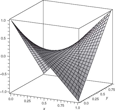
Example 1.9 For an example of the use of von Neumann’s theorem, suppose we look at
![]()
This function has fxx = 0 ≤ 0, fyy = 0 ≥ 0, so it is convex in y for each x and concave in x for each y. Since (x, y) ![]() [0, 1] × [0, 1], and the square is closed and bounded, von Neumann’s theorem guarantees the existence of a saddle point for this function. To find it, solve fx = fy = 0 to get x = y =
[0, 1] × [0, 1], and the square is closed and bounded, von Neumann’s theorem guarantees the existence of a saddle point for this function. To find it, solve fx = fy = 0 to get x = y = ![]() . The Hessian for f, which is the matrix of second partial derivatives, is given by
. The Hessian for f, which is the matrix of second partial derivatives, is given by
![]()
Since (H) = −16 < 0 we are guaranteed by elementary calculus that (x = ![]() , y =
, y = ![]() ) is an interior saddle for f. Figure 1.5 is a picture of f:
) is an interior saddle for f. Figure 1.5 is a picture of f:
Incidentally, another way to write our example function would be
![]()
We will see that f(x, y) is constructed from a matrix game in which player I uses the variable mixed strategy X = (x, 1 − x), and player II uses the variable mixed strategy Y = (y, 1 − y).
FIGURE 1.5 A function with a saddle point at (1/2, 1/2).
Obviously, not all functions will have saddle points. For instance, you will show in an exercise that g(x, y) = (x - y)2 is not concave–convex and in fact does not have a saddle point in [0, 1] × [0, 1].
1.2.1 PROOF OF VON NEUMANN’S MINIMAX THEOREM (OPTIONAL)
Many generalizations of von Neumann’s theorem have been given.5 There are also lots of proofs. We will give a sketch of two6 of them for your choice; one of them is hard, and the other is easy. You decide which is which. For the time being you can safely skip these proofs because they won’t be used elsewhere.
Proof 1. Define the sets of points where the min or max is attained by
![]()
and
![]()
By the assumptions on f, C, D, these sets are nonempty, closed, and convex. For instance, here is why Bx is convex. Take ![]() and let λ
and let λ ![]() (0, 1). Then
(0, 1). Then
![]()
But ![]() as well, and so they must be equal. This means that
as well, and so they must be equal. This means that ![]()
Now define g(x, y) ![]() Ay × Bx, which takes a point (x, y)
Ay × Bx, which takes a point (x, y) ![]() C × D and gives the set Ay × Bx. This function satisfies the continuity properties required by Kakutani’s theorem, which is presented below. Furthermore, the sets Ay × Bx are nonempty, convex, and closed, and so Kakutani’s theorem says that there is a point (x*, y*)
C × D and gives the set Ay × Bx. This function satisfies the continuity properties required by Kakutani’s theorem, which is presented below. Furthermore, the sets Ay × Bx are nonempty, convex, and closed, and so Kakutani’s theorem says that there is a point (x*, y*) ![]() g(x*, y*) = Ay* × Bx*.
g(x*, y*) = Ay* × Bx*.
Writing out what this says, we get
![]()
so that

and
![]()
This says that (x*, y*) is a saddle point and v = v+=v− = f(x*, y*). ![]()
Here is the version of Kakutani’s theorem that we are using.
Theorem 1.2.4 (Kakutani) Let C be a closed, bounded, and convex subset of ![]() n, and let g be a point (in C) to set (subsets of C) function. Assume that for each x
n, and let g be a point (in C) to set (subsets of C) function. Assume that for each x ![]() C, the set g(x) is nonempty and convex. Also assume that g is (upper semi)continuous7 Then there is a point x*
C, the set g(x) is nonempty and convex. Also assume that g is (upper semi)continuous7 Then there is a point x* ![]() C satisfying x*
C satisfying x* ![]() g(x*).
g(x*).
This theorem makes the proof of the minimax theorem fairly simple. Kakutani’s theorem is a fixed-point theorem with a very wide scope of uses and applications. A fixed-point theorem gives conditions under which a function has a point x* that satisfies f(x*) = x*, so f fixes the point x*. In fact, later we will use Kakutani’s theorem to show that a generalized saddle point, called Nash equilibrium, is a fixed point.
Now for the second proof of von Neumann’s theorem, we sketch a proof using only elementary properties of convex functions and some advanced calculus. You may refer to Devinatz (1968) for all the calculus used in this book.
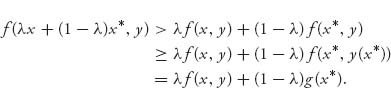
Proof 2. 1. Assume first that f is strictly concave–convex, meaning that
The advantage of doing this is that for each x ![]() C there is one and only one y = y(x)
C there is one and only one y = y(x) ![]() D (y depends on the choice of x) so that
D (y depends on the choice of x) so that
![]()
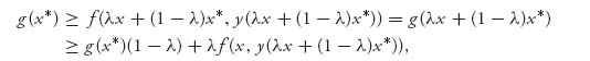
This defines a function g: C → ![]() that is continuous (since f is continuous on the closed bounded sets C × D and thus is uniformly continuous). Furthermore, g(x) is concave since
that is continuous (since f is continuous on the closed bounded sets C × D and thus is uniformly continuous). Furthermore, g(x) is concave since
![]()
So, there is a point x* ![]() C at which g achieves its maximum:
C at which g achieves its maximum:
![]()
2. Let x ![]() C and y
C and y ![]() D be arbitrary. Then, for any 0 < λ < 1, we obtain
D be arbitrary. Then, for any 0 < λ < 1, we obtain
Now take y = y (λ x + (1 − λ)x*) ![]() D to get
D to get
where the first inequality follows from the fact that g(x*) ≥ g(x), ![]() x
x ![]() C. As a result, we have
C. As a result, we have
![]()
or
![]()
3. Sending λ → 0, we see that λ x + (1 − λ) x* → x* and y(λ x + (1 − λ)x*) → y(x*).
We obtain
![]()
Consequently, with y* = y(x*)
![]()
In addition, since ![]() for all y
for all y ![]() D, we get
D, we get
![]()
This says that (x*, y*) is a saddle point and the minimax theorem holds, since
![]()
and so we have equality throughout because the right side is always less than the left side.
4. The last step would be to get rid of the assumption of strict concavity and convexity. Here is how it goes. For ![]() > 0, set
> 0, set
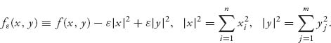
This function will be strictly concave–convex, so the previous steps apply to f![]() . Therefore, we get a point (x
. Therefore, we get a point (x![]() , y
, y![]() )
) ![]() C × D so that v
C × D so that v![]() = f
= f![]() (x
(x![]() , y
, y![]() ) and
) and
![]()
Since ![]() and
and ![]() we get
we get
![]()
Since the sets C, D are closed and bounded, we take a sequence ![]() → 0, x
→ 0, x![]() → x*
→ x* ![]() C, y
C, y![]() → y*
→ y* ![]() D, and also v
D, and also v![]() → v
→ v ![]()
![]() . Sending
. Sending ![]() → 0, we get
→ 0, we get
![]()
This says that v+ = v− = v and (x*, y*) is a saddle point. ![]()
Problems
1.14 Let f(x, y) = x2 + y2, C = D = [−1, 1]. Find v+ = min y![]() D max x
D max x ![]() Cf(x, y) and v− = max x
Cf(x, y) and v− = max x ![]() C min y
C min y ![]() D f(x, y).
D f(x, y).
14.5 Let f(x, y) = y2 − x2, C = D = [−1, 1].
1.16 Let f(x, y) = (x − y)2, C = D = [−1, 1]. Find v+ = min y ![]() D} max x
D} max x ![]() C f(x, y) and v− = max x
C f(x, y) and v− = max x ![]() C min y
C min y ![]() D f(x, y).
D f(x, y).
1.17 Show that for any matrix An×m, the function ![]() defined by
defined by ![]() is convex in y = (y1, ..., ym) and concave in x = (x1, ..., xn). In fact, it is bilinear.
is convex in y = (y1, ..., ym) and concave in x = (x1, ..., xn). In fact, it is bilinear.
1.18 Show that for any real-valued function f = f(x, y), x ![]() C, y
C, y ![]() D, where C and D are any old sets, it is always true that
D, where C and D are any old sets, it is always true that
![]()
Verify that if there is x* ![]() C and y*
C and y* ![]() D and a real number v so that
D and a real number v so that
![]()
then
1.20 Suppose that f: [0, 1] × [0, 1] → ![]() is strictly concave in x
is strictly concave in x ![]() [0, 1] and strictly convex in y
[0, 1] and strictly convex in y ![]() [0, 1] and continuous. Then there is a point (x*, y*) so that
[0, 1] and continuous. Then there is a point (x*, y*) so that
![]()
In fact, define y = ![]() (x) as the function so that f(x,
(x) as the function so that f(x, ![]() (x))= miny f(x, y). This function is well defined and continuous by the assumptions. Also define the function x =
(x))= miny f(x, y). This function is well defined and continuous by the assumptions. Also define the function x = ![]() (y) by f(
(y) by f(![]() (y), y) = max x f(x, y). The new function g(x) =
(y), y) = max x f(x, y). The new function g(x) = ![]() (
(![]() (x)) is then a continuous function taking points in [0, 1] and resulting in points in [0, 1]. There is a theorem, called the Brouwer fixed-point theorem, which now guarantees that there is a point x*
(x)) is then a continuous function taking points in [0, 1] and resulting in points in [0, 1]. There is a theorem, called the Brouwer fixed-point theorem, which now guarantees that there is a point x* ![]() [0, 1] so that g(x *) = x*. Set y* =
[0, 1] so that g(x *) = x*. Set y* = ![]() (x*). Verify that (x*, y*) satisfies the requirements of a saddle point for f.
(x*). Verify that (x*, y*) satisfies the requirements of a saddle point for f.
1.3 Mixed Strategies
von Neumann’s theorem suggests that if we expect to formulate a game model that will give us a saddle point, in some sense, we need convexity of the sets of strategies, whatever they may be, and concavity–convexity of the payoff function, whatever it may be.
Now let’s review a bit. In most two-person zero sum games, a saddle point in pure strategies will not exist because that would say that the players should always do the same thing. Such games, which include 2 × 2 Nim, tic-tac-toe, and many others, are not interesting when played over and over. It seems that if a player should not always play the same strategy, then there should be some randomness involved, because otherwise the opposing player will be able to figure out what the first player is doing and take advantage of it. A player who chooses a pure strategy randomly chooses a row or column according to some probability process that specifies the chance that each pure strategy will be played. These probability vectors are called mixed strategies, and will turn out to be the correct class of strategies for each of the players.
Definition 1.3.1 A mixed strategy is a vector (or 1 × n matrix) X = (x1, ..., xn) for player I and Y = (y1, ..., ym) for player II, where
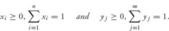
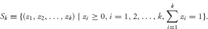
The components xi represent the probability that row i will be used by player I, so xi = Prob(I uses row i}), and yj the probability column j will be used by player II, that is, yj = Prob (II uses row j). Denote the set of mixed strategies with k components by
In this terminology, a mixed strategy for player I is any element X ![]() Sn and for player II any element Y
Sn and for player II any element Y ![]() Sm. A pure strategy X
Sm. A pure strategy X ![]() Sn is an element of the form X = (0, 0, ..., 0, 1, 0, ..., 0), which represents always playing the row corresponding to the position of the 1 in X.
Sn is an element of the form X = (0, 0, ..., 0, 1, 0, ..., 0), which represents always playing the row corresponding to the position of the 1 in X.
If player I uses the mixed strategy X = (x1, ..., xn) ![]() Sn then she will use row i on each play of the game with probability xi. Every pure strategy is also a mixed strategy by choosing all the probability to be concentrated at the row or column that the player wants to always play. For example, if player I wants to always play row 3, then the mixed strategy she would choose is X = (0, 0, 1, 0, ..., 0). Therefore, allowing the players to choose mixed strategies permits many more choices, and the mixed strategies make it possible to mix up the pure strategies used. The set of mixed strategies contains the set of all pure strategies in this sense, and it is a generalization of the idea of strategy.
Sn then she will use row i on each play of the game with probability xi. Every pure strategy is also a mixed strategy by choosing all the probability to be concentrated at the row or column that the player wants to always play. For example, if player I wants to always play row 3, then the mixed strategy she would choose is X = (0, 0, 1, 0, ..., 0). Therefore, allowing the players to choose mixed strategies permits many more choices, and the mixed strategies make it possible to mix up the pure strategies used. The set of mixed strategies contains the set of all pure strategies in this sense, and it is a generalization of the idea of strategy.
Now, if the players use mixed strategies the payoff can be calculated only in the expected sense. That means the game payoff will represent what each player can expect to receive and will actually receive on average only if the game is played many, many times. More precisely, we calculate as follows.
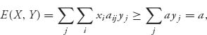
Definition 1.3.2 Given a choice of mixed strategy X ![]() Sn for player I and Y
Sn for player I and Y ![]() Sm for player II, chosen independently, the expected payoff to player I of the game is
Sm for player II, chosen independently, the expected payoff to player I of the game is
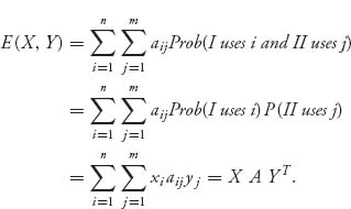
In a zero sum two-person game, the expected payoff to player II would be −E(X, Y). The independent choice of strategy by each player justifies the fact that
![]()
The expected payoff to player I, if I chooses X ![]() Sn and II chooses Y
Sn and II chooses Y ![]() Sm, will be
Sm, will be
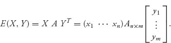
This is written in matrix form with YT denoting the transpose of Y, and where X is 1 × n, A is n × m, and YT is m × 1. If the game is played only once, player I receives exactly aij, for the pure strategies i and j for that play. Only when the game is played many times can player I expect8 to receive approximately E(X, Y).
In the mixed matrix zero sum game the goals now are that player I wants to maximize his expected payoff and player II wants to minimize the expected payoff to I.
We may define the upper and lower values of the mixed game as
![]()
However, we will see shortly that this is really not needed because it is always true that v+ = v− when we allow mixed strategies. Of course, we have seen that this is not true when we permit only pure strategies.
Now we can define what we mean by a saddle point in mixed strategies.
Definition 1.3.3 A saddle point in mixed strategies is a pair (X*, Y*) of probability vectors X* ![]() Sn, Y*
Sn, Y* ![]() Sm, which satisfies
Sm, which satisfies
![]()
If player I decides to use a strategy other than X* but player II still uses Y*, then I receives an expected payoff smaller than that obtainable by sticking with X*. A similar statement holds for player II. (X*, Y*) is an equilibriumin this sense.
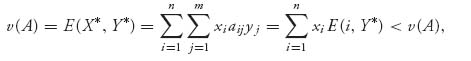
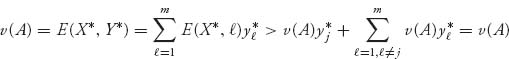
Does a game with matrix A have a saddle point in mixed strategies? von Neumann’s minimax theorem, Theorem 1.2.3, tells us the answer is Yes. All we need to do is define the function f(X, Y)![]() E(X, Y) = XAYT and the sets Sn for X, and Sm for Y. For any n × m matrix A, this function is concave in X and convex in Y. Actually, it is even linear in each variable when the other variable is fixed. Recall that any linear function is both concave and convex, so our function f is concave–convex and certainly continuous. The second requirement of von Neumann’s theorem is that the sets Sn and Sm be convex sets. This is very easy to check and we leave that as an exercise for the reader. These sets are also closed and bounded. Consequently, we may apply the general Theorem 1.2.3 to conclude the following.
E(X, Y) = XAYT and the sets Sn for X, and Sm for Y. For any n × m matrix A, this function is concave in X and convex in Y. Actually, it is even linear in each variable when the other variable is fixed. Recall that any linear function is both concave and convex, so our function f is concave–convex and certainly continuous. The second requirement of von Neumann’s theorem is that the sets Sn and Sm be convex sets. This is very easy to check and we leave that as an exercise for the reader. These sets are also closed and bounded. Consequently, we may apply the general Theorem 1.2.3 to conclude the following.
Theorem 1.3.4 For any n × m matrix A, we have
![]()
The common value is denoted v(A), or value(A), and that is the value of the game. In addition, there is at least one saddle point X* ![]() Sn, Y*
Sn, Y* ![]() Sm so that
Sm so that
![]()
We have already indicated that the proof is a special case for any concave–convex function. Here is a proof that works specifically for matrix games. Since for any function it is true that min max ≥ max min, only the reverse inequality needs to be established. This proof may be skipped.
Proof. The proof is based on a theorem called the separating hyperplane theorem that says that two convex sets can be strictly separated. Here is the separating theorem. ![]()
Theorem 1.3.5 Suppose C ![]()
![]() n is a closed, convex set such that
n is a closed, convex set such that ![]() Then
Then ![]() and C can be strictly separated by a hyperplane. That is, there is a
and C can be strictly separated by a hyperplane. That is, there is a ![]() and a constant c > 0 such that > so
and a constant c > 0 such that > so ![]() so
so![]() lies on one side of the hyperplane
lies on one side of the hyperplane ![]() and C lies on the other side.
and C lies on the other side.
This isn’t hard to prove but we will skip it since geometrically it seems obvious. Now to prove the von Neumann theorem for matrix games, we start with the fact that
![]()
The upper value is always greater than the lower value. Now suppose v− < v+. Then there is a constant γ so that v− < γ < v+. Since ![]() for any constant, we may as well assume that γ = 0 by replacing A with A − γ if necessary.
for any constant, we may as well assume that γ = 0 by replacing A with A − γ if necessary.
Now consider the set
![]()
It is easy to check that this is a closed convex set.
We claim that ![]()
![]() K. In fact, if
K. In fact, if ![]()
![]() K, then there is Y
K, then there is Y ![]() Sm and
Sm and ![]() ≥
≥ ![]() so that
so that
![]()
for any X ![]() Sn. But then
Sn. But then
![]()
which contradicts v+ > 0 > v−. Applying the separating hyperplane theorem, we have the existence of a ![]()
![]()
![]() n and a constant c > 0 so that
n and a constant c > 0 so that ![]() ˙
˙ ![]() > c > 0 for all
> c > 0 for all ![]()
![]() K. Writing out what this means
K. Writing out what this means
![]()
We will show that using ![]() we may construct a mixed strategy for player I.
we may construct a mixed strategy for player I.
First, suppose that some component pi < 0 of ![]() . This would be a bad for a strategy so we’ll show it can’t happen. Simply choose
. This would be a bad for a strategy so we’ll show it can’t happen. Simply choose ![]() = (0, ..., z, 0, ..., 0)
= (0, ..., z, 0, ..., 0) ![]()
![]() n with z in the ith position and we get
n with z in the ith position and we get
![]()
but if we let z → ![]() , since pi < 0 there is no way this will stay positive. Hence, all components of
, since pi < 0 there is no way this will stay positive. Hence, all components of ![]() must be nonnegative,
must be nonnegative, ![]() ≥
≥ ![]() .
.
Another thing that could go wrong is if ![]() =
= ![]() . But that instantly contradicts
. But that instantly contradicts ![]() AYT +
AYT + ![]() ˙
˙ ![]() > c > 0. The conclusion is that if we define
> c > 0. The conclusion is that if we define
then X* ![]() Sn is a bona fide strategy for player I. We then get
Sn is a bona fide strategy for player I. We then get
![]()
Finally, we now have
![]()
That is, ![]() a contradiction to the fact v− < 0.
a contradiction to the fact v− < 0.
Remark The theorem says there is always at least one saddle point in mixed strategies. There could be more than one. If the game happens to have a saddle point in pure strategies, we should be able to discover that by calculating v+ and v− using the columns and rows as we did earlier. This is the first thing to check. The theorem is not used for finding the optimal pure strategies, and while it states that there is always a saddle point in mixed strategies, it does not give a way to find them. The next theorem is a step in that direction. First, we need some notation that will be used throughout this book.
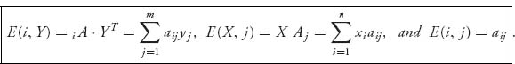
Notation 1.3.6 For an n × m matrix A = (aij) we denote the jth column vector of A by Aj and the ith row vector of A by iA. So
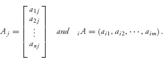
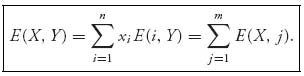
If player I decides to use the pure strategy X = (0, ..., 0, 1, 0, ..., 0) with row i used 100% of the time and player II uses the mixed strategy Y, we denote the expected payoff by E (i, Y) = iA ˙ YT. Similarly, if player II decides to use the pure strategy Y = (0, ..., 0, 1, 0, ..., 0) with column j used 100% of the time, we denote the expected payoff by E(X, j) = X A j. We may also write
Note too that
The von Neumann minimax theorem tells us that every matrix game has a saddle point in mixed strategies. That is there are always strategies X* ![]() Sn, Y*
Sn, Y* ![]() Sm so that
Sm so that
![]()
A saddle point means that if one player deviates from using her part of the saddle, then the other player can do better. It is an equilibrium in that sense. The question we deal with next is how to find a saddle.
The next lemma says that mixed against all pure is as good as mixed against mixed. This lemma will be used in several places in the discussion following. It shows that if an inequality holds for a mixed strategy X for player I, no matter what column is used for player II, then the inequality holds even if player II uses a mixed strategy.
More precisely,
Lemma 1.3.7 If X ![]() Sn is any mixed strategy for player I and a is any number so that
Sn is any mixed strategy for player I and a is any number so that ![]() then for any Y
then for any Y ![]() Sm, it is also true that E(X, Y) ≥ a.
Sm, it is also true that E(X, Y) ≥ a.
Similarly, if Y ![]() Sm is any mixed strategy for player II and a is any number so that E(i, Y) ≤ a,
Sm is any mixed strategy for player II and a is any number so that E(i, Y) ≤ a, ![]() i = 1, 2, ..., n, then for any X
i = 1, 2, ..., n, then for any X ![]() Sn, it is also true that E(X, Y) ≤ a.
Sn, it is also true that E(X, Y) ≤ a.
Here is why. The inequality E(X, j) ≥ a means that ![]() i xi aij ≥ a. Now multiply both sides by yj ≥ 0 and sum on j to see that
i xi aij ≥ a. Now multiply both sides by yj ≥ 0 and sum on j to see that
because ![]() j yj = 1. Basically, this result says that if X is a good strategy for player I when player II uses any pure strategy, then it is still a good strategy for player I even if player II uses a mixed strategy. Seems obvious.
j yj = 1. Basically, this result says that if X is a good strategy for player I when player II uses any pure strategy, then it is still a good strategy for player I even if player II uses a mixed strategy. Seems obvious.
Our next theorem gives us a way of finding the value and the optimal mixed strategies. From now on, whenever we refer to the value of a game, we are assuming that the value is calculated using mixed strategies.
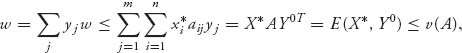
Theorem 1.3.8 Let A = (aij) be an n × m game with value v(A). Let w be a real number. Let X* ![]() Sn be a strategy for player I and Y *
Sn be a strategy for player I and Y * ![]() Sm be a strategy for player II.
Sm be a strategy for player II.
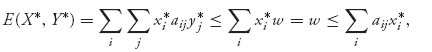
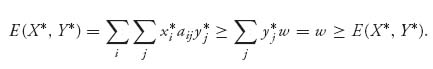
Part (c) of the theorem is particularly useful because it gives us a system of inequalities involving v(A), X*, and Y*. In fact, the main result of the theorem can be summarized in the following statement.
A number v is the value of the game with matrix A and (X*, Y*) is a saddle point in mixed strategies if and only if
(1.3)![]()
Remarks 1. One important way to use the theorem is as a verification tool. If someone says that v is the value of a game and Y is optimal for player II, then you can check it by ensuring that E(i, Y) ≤ v for every row. If even one of those is not true, then either Y is not optimal for II, or v is not the value of the game. You can do the same thing given v and an X for player I. For example, let’s verify that for the matrix

the optimal strategies are X* = Y* = (![]() ,
, ![]() ) and the value of the game is v(A) =
) and the value of the game is v(A) = ![]() . All we have to do is check that
. All we have to do is check that
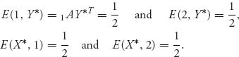
Then the theorem guarantees that v(A) = ![]() and (X*, Y*) is a saddle and you can take it to the bank. Similarly, if we take X = (
and (X*, Y*) is a saddle and you can take it to the bank. Similarly, if we take X = (![]() ,
, ![]() ), then E(X, 2) =
), then E(X, 2) = ![]() <
< ![]() , and so, since v =
, and so, since v = ![]() is the value of the game, we know that X is not optimal for player I.
is the value of the game, we know that X is not optimal for player I.
Proof of Theorem 1.3.8
(a) Suppose
Let Y0 = (yj) ![]() Sm be an optimal mixed strategy for player II. Multiply both sides by yj and sum on j to see that
Sm be an optimal mixed strategy for player II. Multiply both sides by yj and sum on j to see that
since ![]() j yj = 1, and since E(X, Y0) ≤ v(A) for all X
j yj = 1, and since E(X, Y0) ≤ v(A) for all X ![]() Sn.
Sn.
Part (b) follows in the same way as (a). ![]()
(c) If ![]() we have
we have
and
This says that w = E(X*, Y*). So now we have E(i, Y*) ≤ E(X*, Y*) ≤ E(X*, j) for any row i and column j. Taking now any strategies X ![]() Sn and Y
Sn and Y ![]() Sm and using Lemma 1.3.7, we get E(X, Y*) ≤ E(X*, Y*) ≤ E(X*, Y) so that (X*, Y*) is a saddle point and v(A) = E(X*, Y*)= w.
Sm and using Lemma 1.3.7, we get E(X, Y*) ≤ E(X*, Y*) ≤ E(X*, Y) so that (X*, Y*) is a saddle point and v(A) = E(X*, Y*)= w. ![]()
(d) Let Y0 ![]() Sm be optimal for player II. Then E(i, Y0) ≤ v(A) ≤ E(X*, j), for all rows i and columns j, where the first inequality comes from the definition of optimal for player II. Now use part (c) of the theorem to see that X* is optimal for player I. The second part of (d) is similar.
Sm be optimal for player II. Then E(i, Y0) ≤ v(A) ≤ E(X*, j), for all rows i and columns j, where the first inequality comes from the definition of optimal for player II. Now use part (c) of the theorem to see that X* is optimal for player I. The second part of (d) is similar. ![]()
(e) We begin by establishing that minY E(X, Y) = minj E(X, j) for any fixed X ![]() Sn. To see this, since every pure strategy is also a mixed strategy, it is clear that minY E(X, Y) ≤ minj E(X, j). Now set a = minj E(X, j). Then
Sn. To see this, since every pure strategy is also a mixed strategy, it is clear that minY E(X, Y) ≤ minj E(X, j). Now set a = minj E(X, j). Then
since E(X, j) ≥ a for each j = 1, 2, ..., m. Consequently, minY E(X, Y) ≥ a, and putting the two inequalities together, we conclude that minY E(X, Y) = minj E(X, j).
Using the definition of v(A), we then have
![]()
In a similar way, we can also show that v(A) = minY maxi E(i, Y). Consequently,
![]()
If X* is optimal for player I, then
![]()
On the other hand, if v(A) ≤ minj E(X*, j), then v(A) ≤ E(X*, j) for any column, and so v(A) ≤ E(X*, Y) for any Y ![]() Sm, by Lemma 1.3.7, which implies that X* is optimal for player I.
Sm, by Lemma 1.3.7, which implies that X* is optimal for player I. ![]()
The proof of part (e) contained a result important enough to separate into the following corollary. It says that only one player really needs to play mixed strategies in order to calculate v(A). It also says that v(A) is always between v− and v+.
Corollary 1.3.9
![]()
In addition, v− = maxi minj aij ≤ v(A) ≤ minj maxi aij = v+.
Be aware of the fact that not only are the min and max in the corollary being switched but also the sets over which the min and max are taken are changing. The second part of the corollary is immediate from the first part since
![]()
and
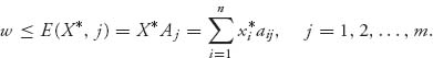
Now let’s use the theorem to see how we can compute the value and strategies for some games. Essentially, we consider the system of inequations
![]()
along with the condition x1 + … + xn = 1. We need the last equation because v is also an unknown. If we can solve these inequalities and the xi variables turn out to be nonnegative, then that gives us a candidate for the optimal mixed strategy for player I, and our candidate for the value v = v(A). Once we know, or think we know v(A), then we can solve the system E(i, Y) ≤ v(A) for player II’s Y strategy. If all the variables yj are nonnegative and sum to one, then Equation (1.3) tells us that we have the solution in hand and we are done.
Example 1.10 We start with a simple game with matrix
Note that v− = − 1 and v+ = 3, so this game does not have a saddle in pure strategies. We will use parts (c) and (e) of Theorem 1.3.8 to find the mixed saddle. Suppose that X = (x, 1 − x) is optimal and v = v(A) is the value of the game. Then v ≤ E(X, 1) and v ≤ E(X, 2), which gives us v ≤ 4x − 1 and v ≤ −10x + 9. If we can find a solution of these, with equality instead of inequality, and it is valid (i.e., 0 ≤ x ≤ 1), then we will have found the optimal strategy for player I and v(A) = v. So, first try replacing all inequalities with equalities. The equations become
![]()
and can be solved for x and v to get ![]() and
and ![]() Since
Since ![]() is a legitimate strategy and
is a legitimate strategy and ![]() satisfies the conditions in Theorem 1.3.8, we know that X is optimal. Similarly
satisfies the conditions in Theorem 1.3.8, we know that X is optimal. Similarly ![]() is optimal for player II.
is optimal for player II.
Example 1.11 Evens and Odds Revisited. In the game of evens or odds, we came up with the game matrix
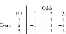
We calculated that v− = − 1 and v+ = + 1, so this game does not have a saddle point using only pure strategies. But it does have a value and saddle point using mixed strategies. Suppose that v is the value of this game and (X* = (x1, x2, x3), Y* = (y1, y2, y3)) is a saddle point. According to Theorem 1.3.8, these quantities should satisfy
![]()
Using the values from the matrix, we have the system of inequalities
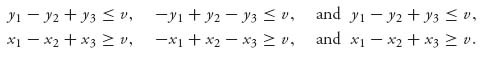
Let’s go through finding only the strategy X* since finding Y* is similar. We are looking for numbers x1, x2, x3 and v satisfying x1 − x2 + x3 ≥ v, − x1 + x2 − x3 ≥ v, as well as x1 + x2 + x3 = 1 and xi ≥ 0, i = 1, 2, 3. But then x1 = 1 − x2 − x3, and so
![]()
If v ≥ 0, this says that in fact v = 0 and then x2 = ![]() . Let’s assume then that v = 0 and x2=
. Let’s assume then that v = 0 and x2= ![]() . This would force x1+ x3 =
. This would force x1+ x3 = ![]() as well.
as well.
Instead of substituting for x1, substitute x2 = 1 − x1 − x3 hoping to be able to find x1 or x3. You would see that we would once again get x1 + x3 = ![]() . Something is going on with x1 and x3, and we don’t seem to have enough information to find them. But we can see from the matrix that it doesn’t matter whether player I shows one or three fingers! The payoffs in all cases are the same. This means that row 3 (or row 1) is a redundant strategy and we might as well drop it. (We can say the same for column 1 or column 3.) If we drop row 3, we perform the same set of calculations but we quickly find that x2 =
. Something is going on with x1 and x3, and we don’t seem to have enough information to find them. But we can see from the matrix that it doesn’t matter whether player I shows one or three fingers! The payoffs in all cases are the same. This means that row 3 (or row 1) is a redundant strategy and we might as well drop it. (We can say the same for column 1 or column 3.) If we drop row 3, we perform the same set of calculations but we quickly find that x2 = ![]() = x1. Of course, we assumed that v ≥ 0 to get this but now we have our candidates for the saddle points and value, namely, v = 0, X* = (
= x1. Of course, we assumed that v ≥ 0 to get this but now we have our candidates for the saddle points and value, namely, v = 0, X* = (![]() ,
, ![]() , 0) and also, in a similar way Y* = (
, 0) and also, in a similar way Y* = (![]() ,
, ![]() , 0). Check that with these candidates the inequalities of Theorem 40 are satisfied and so they are the actual value and saddle.
, 0). Check that with these candidates the inequalities of Theorem 40 are satisfied and so they are the actual value and saddle.
However, it is important to remember that with all three rows and columns, the theorem does not give a single characterization of the saddle point. Indeed, there are an infinite number of saddle points, X* = (x1, ![]() ,
, ![]() − x1), 0 ≤ x1 ≤
− x1), 0 ≤ x1 ≤ ![]() and Y* = (y1,
and Y* = (y1, ![]() ,
, ![]() − y1), 0 ≤ y1 ≤
− y1), 0 ≤ y1 ≤ ![]() . Nevertheless, there is only one value for this, or any matrix game, and it is v = 0 in the game of odds and evens.
. Nevertheless, there is only one value for this, or any matrix game, and it is v = 0 in the game of odds and evens.
Later we will see that the theorem gives a method for solving any matrix game if we pair it up with another theory, namely, linear programming, which is a way to optimize a linear function over a set with linear constraints. Linear programming will accommodate the more difficult problem of solving a system of inequalities.
Here is a summary of the basic results in two-person zero sum game theory that we may use to find optimal strategies.
1.3.1 PROPERTIES OF OPTIMAL STRATEGIES
![]()
Thus, if any optimal mixed strategy for a player has a strictly positive probability of using a row or a column, then that row or column played against any optimal opponent strategy will yield the value. This result is also called the Equilibrium Theorem.
![]()
Remark Property 3 give us a way of solving games algebraically without having to solve inequalities. Let’s list this as a proposition.
Proposition 1.3.10 The value of the game, v(A), and the optimal strategies X* = (x*1, ..., x*n) for player I and Y* = (y*1, ..., y*m) for player II must satisfy the system of equations E(i, Y*) = v(A) for each row with xi* > 0 and E(X*, j) = v(A) for every column j with yj* > 0. In particular, if xi > 0, xk > 0, then E(i, Y*) = E(k, Y*). Similarly, if y*j > 0, y*e > 0, then E(X*, j) = E(X* e).
Of course, we generally do not know v(A), X*, and Y* ahead of time, but if we can solve these equations and then verify optimality using the properties, we have a plan for solving the game.
Observe the very important fact that if you assume row i is used by player I, then E(i, Y) = v is an equation for the unknown Y. Similarly, if column j is used by player II, then E(X, j) = v is an equation for the unknown X. In other words, the assumption about one player leads to an equation for the other player.
Proof of Property 3. If it happens that (X*, Y*) are optimal and there is a component of X* = ![]() but E(k, Y*) < v(A), then multiplying both sides of E(k, Y*) < v(A) by
but E(k, Y*) < v(A), then multiplying both sides of E(k, Y*) < v(A) by ![]() yields
yields ![]() E (k, Y*) <
E (k, Y*) < ![]() v(A). Now, it is always true that for any row i = 1, 2, ..., n,
v(A). Now, it is always true that for any row i = 1, 2, ..., n,
![]()
But then, because v(A) > E(k, Y*) and ![]() > 0, by adding, we get
> 0, by adding, we get
We see that, under the assumption E(k, Y*) < v(A), we have
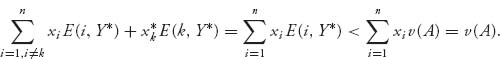
which is a contradiction. But this means that if ![]() > 0 we must have E(k, Y*) = v(A).
> 0 we must have E(k, Y*) = v(A).
Similarly, suppose E(X*, j) > v(A) where Y* = (y1*, ..., yj*, ..., ym*), yj* > 0. Then
again a contradiction. Hence, E(X*, j) > v(A) ![]() yj* = 0.
yj* = 0. ![]()
We will not prove properties (5) and (6) since we really do not use these facts.
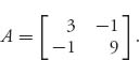
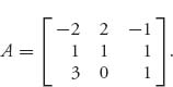
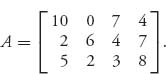
Example 1.12 Let’s consider the game with matrix
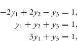
We solve this game by using the properties. First, it appears that every row and column should be used in an optimal mixed strategy for the players, so we conjecture that if X = (x1, x2, x3) is optimal, then xi > 0. This means, by property 3, that we have the following system of equations for Y = (y1, y2, y3):
A small amount of algebra gives the solution y1 = y2 = y3 = ![]() and v = 2. But, then, Theorem 1.3.8 guarantees that Y = (
and v = 2. But, then, Theorem 1.3.8 guarantees that Y = (![]() ,
, ![]() ,
, ![]() ) is indeed an optimal mixed strategy for player II and v(A) = 2 is the value of the game. A similar approach proves that X = (
) is indeed an optimal mixed strategy for player II and v(A) = 2 is the value of the game. A similar approach proves that X = (![]() ,
, ![]() ,
, ![]() ) is also optimal for player I.
) is also optimal for player I.
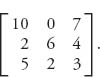
Example 1.13 Let’s consider the game with matrix
We will show that this matrix has an infinite number of mixed saddle points, but only player II has a mixed strategy in which all columns are played. This matrix has a pure saddle point at X* = (0, 1, 0), Y* = (0, 0, 1), and v(A) = 1, as you should verify. We will show that player II has an optimal strategy Y* = (y1, y2, y3), which has yj > 0 for each j. But it is not true that player I has an optimal X = (x1, x2, x3) with xi > 0. In fact, by the equilibrium theorem (Section 1.3.1), property 3, if we assumed that X is optimal and xi > 0, i = 1, 2, 3, then it would have to be true that
because we know that v = 1. However, there is one and only one solution of this system, and it is given by ![]() which is not a strategy. This means that our assumption about the existence of an optimal strategy for player I with xi > 0, i = 1, 2, 3, must be wrong.
which is not a strategy. This means that our assumption about the existence of an optimal strategy for player I with xi > 0, i = 1, 2, 3, must be wrong.
Now assume there is an optimal Y* = (y1, y2, y3), with yj > 0, j = 1, 2, 3. Then E(X*, j) = 1, j = 1, 2, 3, and this leads to the equations for X*= (x1, x2, x3):
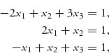
along with x1 + x2 + x3 = 1. The unique solution of these equations is given by X* = (0, 1, 0).
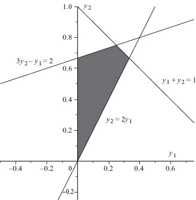
On the other hand, we know that player I has an optimal strategy of X*= (0, 1, 0), and so, by the equilibrium theorem (Section 1.3.1), properties 3 and 5, we know that E(2, Y) = 1, for an optimal strategy for player II, as well as E(1, Y) < 1, and E(3, Y) < 1. We need to look for y1, y2, y3 so that
![]()
We may replace y3 = 1 − y1 − y2 and then get a graph of the region of points satisfying all the inequalities in (y1, y2) space in Figure 1.6.
There are lots of points which work. In particular, Y = (0.15, 0.5, 0.35) will give an optimal strategy for player II in which all yj > 0.
FIGURE 1.6 Optimal strategy set for Y.
1.3.2 DOMINATED STRATEGIES
Computationally, smaller game matrices are better than large matrices. Sometimes, we can reduce the size of the matrix A by eliminating rows or columns (i.e., strategies) that will never be used because there is always a better row or column to use. This is elimination by dominance. We should check for dominance whenever we are trying to analyze a game before we begin because it can reduce the size of a matrix.
For example, if every number in row i is bigger than every corresponding number in row k, specifically aij > akj, j = 1, ..., m, then the row player I would never play row k (since she wants the biggest possible payoff), and so we can drop it from the matrix. Similarly, if every number in column j is less than every corresponding number in column k (i.e., aij < aik, i = 1, ..., n), then the column player II would never play column k (since he wants player I to get the smallest possible payoff), and so we can drop it from the matrix. If we can reduce it to a 2 × m or n × 2 game, we can solve it by a graphical procedure that we will consider shortly. If we can reduce it to a 2 × 2 matrix, we can use the formulas that we derive in the next section. Here is the precise meaning of dominated strategies.
Definition 1.3.11 Row i (strictly) dominates row k if aij > akj for all j = 1, 2, ..., m. This allows us to remove row k. Column j (strictly) dominates column k if aij < aik, i = 1, 2, ..., n. This allows us to remove column k.
Remarks We may also drop rows or columns that are nonstrictly dominated but the resulting matrix may not result in all the saddle points for the original matrix. Finding all of the saddle points is not what we are concerned with so we will use non-strict dominance in what follows.
A row that is dropped because it is strictly dominated is played in a mixed strategy with probability 0. But a row that is dropped because it is equal to another row may not have probability 0 of being played. For example, suppose that we have a matrix with three rows and row 2 is the same as row 3. If we drop row 3, we now have two rows and the resulting optimal strategy will look like X* = (x1, x2) for the reduced game. Then for the original game the optimal strategy could be X* = (x1, x2, 0) or ![]() or in fact X* = (x1, λ x2, (1-λ) x2) for any 0 ≤ λ ≤ 1. The set of all optimal strategies for player I would consist of all X* = (x1, λ x2, (1 − λ) x2) for any 0 ≤ λ ≤ 1, and this is the most general description. A duplicate row is a redundant row and may be dropped to reduce the size of the matrix. But you must account for redundant strategies.
or in fact X* = (x1, λ x2, (1-λ) x2) for any 0 ≤ λ ≤ 1. The set of all optimal strategies for player I would consist of all X* = (x1, λ x2, (1 − λ) x2) for any 0 ≤ λ ≤ 1, and this is the most general description. A duplicate row is a redundant row and may be dropped to reduce the size of the matrix. But you must account for redundant strategies.
Another way to reduce the size of a matrix, which is more subtle, is to drop rows or columns by dominance through a convex combination of other rows or columns. If a row (or column) is (strictly) dominated by a convex combination of other rows (or columns), then this row (column) can be dropped from the matrix. If, for example, row k is dominated by a convex combination of two other rows, say, p and q, then we can drop row k. This means that if there is a constant λ ![]() [0, 1] so that
[0, 1] so that
![]()
then row k is dominated and can be dropped. Of course, if the constant λ = 1, then row p dominates row k and we can drop row k. If λ = 0 then row q dominates row k. More than two rows can be involved in the combination.
For columns, the column player wants small numbers, so column k is dominated by a convex combination of columns p and q if
![]()
It may be hard to spot a combination of rows or columns that dominate, but if there are suspects, the next example shows how to verify it.
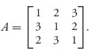
Example 1.14 Consider the 3 × 4 game
It seems that we may drop column 4 right away because every number in that column is larger than each corresponding number in column 2. So now we have
There is no obvious dominance of one row by another or one column by another. However, we suspect that row 3 is dominated by a convex combination of rows 1 and 2. If that is true, we must have, for some 0 ≤ λ ≤ 1, the inequalities
![]()
Simplifying, 5 ≤ 8λ + 2, 2 ≤ 6 − 6 λ, 3 ≤ 3 λ + 4. But this says any ![]() will work. So, there is a λ that works to cause row 3 to be dominated by a convex combination of rows 1 and 2, and row 3 may be dropped from the matrix (i.e., an optimal mixed strategy will play row 3 with probability 0). Remember, to ensure dominance by a convex combination, all we have to show is that there are λs that satisfy all the inequalities. We don’t actually have to find them. So now the new matrix is
will work. So, there is a λ that works to cause row 3 to be dominated by a convex combination of rows 1 and 2, and row 3 may be dropped from the matrix (i.e., an optimal mixed strategy will play row 3 with probability 0). Remember, to ensure dominance by a convex combination, all we have to show is that there are λs that satisfy all the inequalities. We don’t actually have to find them. So now the new matrix is
![]()
Again there is no obvious dominance, but it is a reasonable guess that column 3 is a bad column for player II and that it might be dominated by a combination of columns 1 and 2. To check, we need to have
![]()
These inequalities require that ![]() which is okay. So there are λ’s that work, and column 3 may be dropped. Finally, we are down to a 2 × 2 matrix
which is okay. So there are λ’s that work, and column 3 may be dropped. Finally, we are down to a 2 × 2 matrix

We will see how to solve these small games graphically in Section 1.5. They may also be solved by assuming that each row and column will be used with positive probability and then solving the system of equations. The answer is that the value of the game is ![]() and the optimal strategies for the original game are
and the optimal strategies for the original game are ![]() and
and ![]() You should check that statement with part (c) of the Theorem 1.3.8 or property 1 of (Section 1.3.1).
You should check that statement with part (c) of the Theorem 1.3.8 or property 1 of (Section 1.3.1).
Example 1.15 This example shows that me may lose solutions when we reduce by nonstrict dominance. Consider the game with matrix
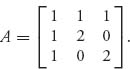
Again there is no obvious dominance, but it is easy to see that row 1 is dominated (nonstrictly) by a convex combination of rows 2 and 3. In fact a1j = ![]() a2j +
a2j + ![]() a3j, j = 1, 2, 3. So if we drop row 1 we next see that column 1 is dominated by a convex combination of columns 2 and 3 and may be dropped. This leaves us with the reduced matrix
a3j, j = 1, 2, 3. So if we drop row 1 we next see that column 1 is dominated by a convex combination of columns 2 and 3 and may be dropped. This leaves us with the reduced matrix ![]() The solution for this reduced game is v = 1, X * = (
The solution for this reduced game is v = 1, X * = (![]() ,
, ![]() ) = Y*, and consequently, a solution of the original game is v(A) = 1, X* = (0,
) = Y*, and consequently, a solution of the original game is v(A) = 1, X* = (0, ![]() ,
, ![]() ) = Y*. However, it is easy to verify that there is in fact a pure saddle point for this game given by X* = (1, 0, 0), Y* = (1, 0, 0) and this is missed by using non-strict domination. Dropping rows or columns that are strictly dominated, however, means that dropped row or column is never played.
) = Y*. However, it is easy to verify that there is in fact a pure saddle point for this game given by X* = (1, 0, 0), Y* = (1, 0, 0) and this is missed by using non-strict domination. Dropping rows or columns that are strictly dominated, however, means that dropped row or column is never played.
Remark Another question which may have occurred to you is When an optimal strategy for a player has a zero component, can you drop that row or column and then solve the reduced matrix?
Answer: No, in general.
Consider the matrix
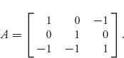
Then a saddle point of this matrix is X* = (0, 1, 0), Y* = (![]() , 0,
, 0, ![]() ), and v(A) = 0. If we drop row 1 (because the optimal strategy for player I has x1 = 0), we get the matrix
), and v(A) = 0. If we drop row 1 (because the optimal strategy for player I has x1 = 0), we get the matrix
![]()
Then ![]() = (1, 0),
= (1, 0), ![]() = (1, 0, 0) is a saddle point for B, v(B) = 0, but
= (1, 0, 0) is a saddle point for B, v(B) = 0, but ![]() is NOT optimal for the original game with matrix A. In fact E(i,
is NOT optimal for the original game with matrix A. In fact E(i, ![]() ) = 1, 0, − 1, for i = 1, 2, 3, and we see that E(i,
) = 1, 0, − 1, for i = 1, 2, 3, and we see that E(i, ![]() ) is not ≤ v(A) = 0, for each i = 1, 2, 3.
) is not ≤ v(A) = 0, for each i = 1, 2, 3.
The only way to be able to carry out the reduction in the statement of the question is if you know that every optimal strategy will have a zero in the same row or column.
1.4 Solving 2 × 2 Games Graphically
If we have a 2 × 2 matrix game, we can always find the optimal mixed strategies using a graph. It also reveals the basic concepts of how each player looks at the payoffs to determine their optimal plays. We will solve an example to illustrate this method.
Suppose that we have the matrix

The first step is that we must check whether there are pure optimal strategies because if there are, then we can’t use the graphical method. It only finds the strategies that are mixed, but we don’t need any fancy methods to find the pure ones. Since v− = 2 and v+ = 3, we know the optimal strategies must be mixed. Now we use Theorem 1.3.8 part (c) to find the optimal strategy X = (x, 1 − x), 0 < x < 1, for player I, and the value of the game v(A). Here is how it goes.
Playing X against each column for player II, we get
![]()
We now plot each of these functions of x on the same graph in Figure 1.7. Each plot will be a straight line with 0 ≤ x ≤ 1.
FIGURE 1.7 X against each column for player II.
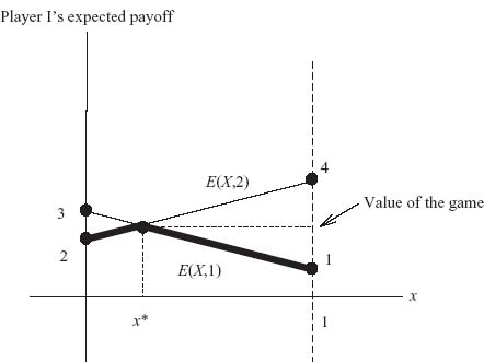
Now, here is how to analyze this graph from player I’s perspective. First, the point at which the two lines intersect is ![]() If player I chooses an x < x*, then the best I can receive is on the highest line when x is on the left of x*. In this case the line is E(X, 1) = x + 3 (1 − x) >
If player I chooses an x < x*, then the best I can receive is on the highest line when x is on the left of x*. In this case the line is E(X, 1) = x + 3 (1 − x) > ![]() . Player I will receive this higher payoff only if player II decides to play column 1. But player II will also have this graph and II will see that if I uses x < x* then II should definitely not use column 1 but should use column 2 so that I would receive a payoff on the lower line E(X, 2)
. Player I will receive this higher payoff only if player II decides to play column 1. But player II will also have this graph and II will see that if I uses x < x* then II should definitely not use column 1 but should use column 2 so that I would receive a payoff on the lower line E(X, 2)![]() . In other words, I will see that II would switch to using column 2 if I chose to use any mixed strategy with x <
. In other words, I will see that II would switch to using column 2 if I chose to use any mixed strategy with x < ![]() . What if I uses an x >
. What if I uses an x > ![]() ? The reasoning is similar; the best I could get would happen if player II chose to use column 2 and then I gets E(X, 2)>
? The reasoning is similar; the best I could get would happen if player II chose to use column 2 and then I gets E(X, 2)>![]() . But I cannot assume that II will play stupidly. Player II will see that if player I chooses to play an x >
. But I cannot assume that II will play stupidly. Player II will see that if player I chooses to play an x > ![]() , II will choose to play column 1 so that I receives some payoff on the line E(X, 1) <
, II will choose to play column 1 so that I receives some payoff on the line E(X, 1) < ![]() .
.
Conclusion: player I, assuming that player II will be doing her best, will choose to play X = (x*, 1 − x*) = (![]() ,
, ![]() ) and then receive exactly the payoff = v(A) =
) and then receive exactly the payoff = v(A) = ![]() . Player I will rationally choose the maximum minimum. The minimums are the bold lines and the maximum minimum is at the intersection, which is the highest point of the bold lines. Another way to put it is that player I will choose a mixed strategy so that she will get
. Player I will rationally choose the maximum minimum. The minimums are the bold lines and the maximum minimum is at the intersection, which is the highest point of the bold lines. Another way to put it is that player I will choose a mixed strategy so that she will get ![]() no matter what player II does, and if II does not play optimally, player I can get more than
no matter what player II does, and if II does not play optimally, player I can get more than ![]() .
.
What should player II do? Before you read the next section, try to figure it out. That will be an exercise.
Problems
1.21 Following the same procedure as that for player I, look at E(i, Y), i = 1, 2. with Y = (y, 1 − y). Graph the lines E(1, Y) = y + 4(1 - y) and E(2, Y) = 3y + 2(1 −y), 0 ≤ y ≤ 1. Now, how does player II analyze the graph to find Y*?
1.22 Find the value and optimal X* for the games with matrices
![]()
What, if anything, goes wrong with (b) if you use the graphical method?
1.23 Curly has two safes, one at home and one at the office. The safe at home is a piece of cake to crack and any thief can get into it. The safe at the office is hard to crack and a thief has only a 15% chance of doing it. Curly has to decide where to place his gold bar (worth 1). On the other hand, if the thief hits the wrong place he gets caught (worth −1 to the thief and +1 to Curly). Formulate this as a two-person zero sum matrix game and solve it using the graphical method.
1.24 Let z be an unknown number and consider the matrices
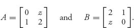
1.25 Suppose that we have the game matrix
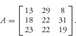
Why can this be reduced to  Now solve the game graphically.
1.26 Two brothers, Curly and Shemp, inherit a car worth 8000 dollars. Since only one of them can actually have the car, they agree they will present sealed bids to buy the car from the other brother. The brother that puts in the highest sealed bid gets the car. They must bid in 1000 dollar units. If the bids happen to be the same, then they flip a coin to determine ownership and no money changes hands. Curly can bid only up to 5000 while Shemp can bid up to 8000.
Find the payoff matrix with Curly as the row player and the payoffs the expected net gain (since the car is worth 8000). Find v−, v+ and use dominance to solve the game.
1.5 Graphical Solution of 2 × m and n × 2 Games
Now we look at the general graphical method that applies whenever one or the other player has only two strategies. This generalizes the 2 × 2 case we looked at briefly.
Consider the game given by
![]()
We denote, as usual, by Aj the jth column of the matrix and iA the i th row. We should always check at the outset whether A has a pure strategy saddle and if so, we don’t need to apply the graphical method (in fact, it could lead to erroneous results). Therefore, assuming that there is no pure saddle, that is, v+ > v−, we may approach this problem as follows.
Since player I has only two pure strategies we solve for I’s optimal strategy first. Suppose that player I chooses a mixed strategy X = (x, 1-x), 0< x < 1, and player II chooses column j. The payoff to player I is E(X, j) = XAj or, written out
![]()
Now, because there are only two rows, a mixed strategy is determined by the choice of the single variable X ![]() [0, 1]. This is perfect for drawing a plot. On a graph (with x on the horizontal axis), y = E(X, j) is a straight line through the two points (0, a2j) and (1, a1j). Now do this for each column j and look at
[0, 1]. This is perfect for drawing a plot. On a graph (with x on the horizontal axis), y = E(X, j) is a straight line through the two points (0, a2j) and (1, a1j). Now do this for each column j and look at
![]()
This is called the lower envelope of all the straight lines associated to each strategy j for player II. Then let 0 ≤ x* ≤ 1 be the point where the maximum of f is achieved:
![]()
This is the maximum minimum of f. Then X* = (x*, 1−x*) is the optimal strategy for player I and f(x*) will be the value of the game v(A). This is shown in Figure 1.8 for a 2 × 3 game.
FIGURE 1.8 Graphical solution for 2 × 3 game.
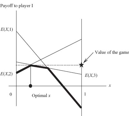
Each line represents the payoff that player I would receive by playing the mixed strategy X = (x, 1 − x), with player II always playing a fixed column. In the figure you can see that if player I decides to play the mixed strategy X1 = (x1, 1 − x1) where x1 is to the left of the optimal value, then player II would choose to play column 2. If player I decides to play the mixed strategy X2 = (x2, 1− x2), where x2 is to the right of the optimal value, then player II would choose to play column 3, up to the point of intersection where E(X, 1) = E(X, 3), and then switch to column 1. This shows how player I should choose x, 0 ≤ x ≤ 1; player I would choose the x that guarantees that she will receive the maximum of all the lower points of the lines. By choosing this optimal value, say, x*, it will be the case that player II would play some combination of columns 2 and 3. It would be a mixture (a convex combination) of the columns because if player II always chose to play, say, column 2, then player I could do better by changing her mixed strategy to a point to the right of the optimal value.
Having found the optimal strategy for player I, we must find the optimal strategy for player II. Again, the graph reveals some information. The only two columns being used in an optimal strategy for player I are columns 2 and 3. This implies, by the properties of optimal strategies (Section 1.3.1), that for this particular graph we can eliminate column 1 and reduce to a 2 × 2 matrix. Now let’s work through a specific example.
Example 1.16 The matrix payoff to player I is
Consider the graph for player I first.
Looking at Figure 1.9, we see that the optimal strategy for I is the x value where the two lower lines intersect and yields X* = ![]() ,
, ![]() ). Also, v(A) = E(X*, 3) = E(X*, 2) = 1. To find the optimal strategy for player II, we see that II will never use the first column. The figure indicates that column 1 is dominated by columns 2 and 3 because it is always above the optimal point. In fact, 1 ≥ − λ + 3(1 − λ) and 3 ≥ 5 λ − 3 (1 − λ) implies that for any
). Also, v(A) = E(X*, 3) = E(X*, 2) = 1. To find the optimal strategy for player II, we see that II will never use the first column. The figure indicates that column 1 is dominated by columns 2 and 3 because it is always above the optimal point. In fact, 1 ≥ − λ + 3(1 − λ) and 3 ≥ 5 λ − 3 (1 − λ) implies that for any ![]() ≤ λ ≤
≤ λ ≤ ![]() the first column is dominated by a convex combination of columns 2 and 3 and may be dropped. So consider the subgame with the first column removed:
the first column is dominated by a convex combination of columns 2 and 3 and may be dropped. So consider the subgame with the first column removed:
Now we will solve this graphically for player II assuming that II uses Y = (y, 1 − y). Consider the payoffs E(1, Y) and E(2, Y), which are the payoffs to I if I plays a row and II plays Y. Player II wants to choose y so that no matter what I does she is guaranteed the smallest maximum. This is now the lowest point of the highest part of the lines in Figure 1.10.
We see that the lines intersect with y* = ![]() . Hence, the optimal strategy for II is Y* = (0,
. Hence, the optimal strategy for II is Y* = (0, ![]() ,
, ![]() ). Of course, we end up with the same v(A) = 1.
). Of course, we end up with the same v(A) = 1.
FIGURE 1.9 Mixed for player I versus player II’s columns.
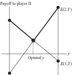
FIGURE 1.10 Mixed for player II versus I’s rows.
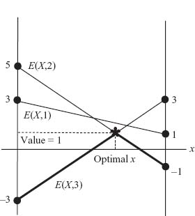
The graphical solution of an n × 2 game is similar to the preceding one except that we begin by finding the optimal strategy for player II first because now II has only two pure strategies. Here is an n × 2 game matrix:
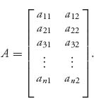
Assume that player II uses the mixed strategy Y = (y, 1 − y), 0 < y < 1. Then II wants to choose y to minimize the quantity:
![]()
For each row i = 1, 2, ..., n, the graph of the payoffs (to player I) E(i, Y) will again be a straight line. We will end up with n lines. Player I will want to go as high as possible, and there is not much player II can do about stopping him from doing that. Player II, playing conservatively, will play the mixed strategy Y, which will give the lowest maximum. The optimal y* will be the point giving the minimum of the upper envelope. Note that this is a guaranteed optimal strategy because if player II deviates from the lowest maximum, player I can do better. Let’s work out another example.
Example 1.17 Let’s consider
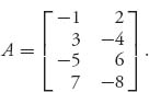
This is a 4 × 2 game without a saddle point in pure strategies since v− = − 1, v+ = 6. There is also no obvious dominance, so we try to solve the game graphically. Suppose that player II uses the strategy Y = (y, 1 − y), then we graph the payoffs E(i, Y), i = 1, 2, 3, 4, as shown in Figure 1.11.
FIGURE 1.11 Mixed for player II versus 4 rows for player I.
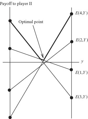
You can see the difficulty with solving games graphically; you have to be very accurate with your graphs. Carefully reading the information, it appears that the optimal strategy for Y will be determined at the intersection point of E(4, Y) = 7y − 8(1 − y) and E(1, Y) = − y + 2(1 −y). This occurs at the point y* = ![]() and the corresponding value of the game will be v(A) =
and the corresponding value of the game will be v(A) = ![]() . The optimal strategy for player II is Y* = (
. The optimal strategy for player II is Y* = (![]() ,
, ![]() ).
).
Since this uses only rows 1 and 4, we may now drop rows 2 and 3 to find the optimal strategy for player I. In general, we may drop the rows (or columns) not used to get the optimal intersection point. Often that is true because the unused rows are dominated, but not always. To see that here, since 3 ≤ 7 ![]() − 1
− 1 ![]() and − 4 ≤ − 8
and − 4 ≤ − 8 ![]() + 2
+ 2 ![]() , we see that row 2 is dominated by a convex combination of rows 1 and 4; so row 2 may be dropped. On the other hand, there is no λ
, we see that row 2 is dominated by a convex combination of rows 1 and 4; so row 2 may be dropped. On the other hand, there is no λ ![]() [0, 1] so that − 5 ≤ 7 λ − 1 (1 − λ) and 6 ≤ − 8 λ + 2 (1 − λ). Row 3 is not dominated by a convex combination of rows 1 and 4, but it is dropped because its payoff line E(3, Y) does not pass through the optimal point.
[0, 1] so that − 5 ≤ 7 λ − 1 (1 − λ) and 6 ≤ − 8 λ + 2 (1 − λ). Row 3 is not dominated by a convex combination of rows 1 and 4, but it is dropped because its payoff line E(3, Y) does not pass through the optimal point.
Considering the matrix using only rows 1 and 4, we now calculate E(X, 1) = − x + 7(1 − x) and E(X, 2) = 2x − 8(1 − x) that intersect at (x = ![]() , v =
, v = ![]() ). We obtain that row 1 should be used with probability
). We obtain that row 1 should be used with probability ![]() and row 4 should be used with probability
and row 4 should be used with probability ![]() , so X* = (
, so X* = (![]() , 0, 0,
, 0, 0, ![]() ). Again, v(A) =
). Again, v(A) = ![]() .
.
A verification that these are indeed optimal uses Theorem 1.3.8c. We check that E(i, Y*) ≤ v(A) ≤ E(X*, j) for all rows and columns. This gives
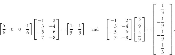
Everything checks.
FIGURE 1.12 A simple poker game. F = fold, B = bet, C = call.
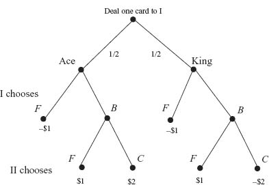
We end this section with a simple analysis of a version of poker, at least a small part of it.
Example 1.18 This is a modified version of the endgame in poker. Here are the rules but it is easier to follow the graphical representation of the game in Figure 1.12. (This is the game in extensive form.)
Why wouldn’t player I immediately fold when he gets dealt a king? Simple, if I folds on a king, he immediately loses $1. Player I is hoping that player II will believe he holds an ace and so will fold if I bets. This is the element of bluffing, because if II calls while I is holding a king, then I must pay II $2.
Now player I has four strategies: FF = fold on ace and fold on king, FB = fold on ace and bet on king, BF = bet on ace and fold on king, and BB = bet on ace and bet on king. Player II has only two strategies, namely, F = fold or C = call. These strategies take into account the fact that player I must have a plan on what to do if he gets an ace or a king, but player II, not knowing the card player I holds, makes a plan based only on whether player I bets, or folds.9
Assuming that the probability of being dealt a king or an ace is ![]() we may calculate the expected reward to player I and get the matrix as follows:
we may calculate the expected reward to player I and get the matrix as follows:
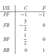
For example, if I plays BF and II plays C, this means that player I will bet if he got an ace, and fold if he got a king. Player II will call no matter what. We calculate the expected payoff to I as ![]() ˙ 2 +
˙ 2 + ![]() (−1) =
(−1) = ![]() . Similarly,
. Similarly,
![]()
and so on. This is a 4 × 2 game that we can solve graphically.
1. The lower and upper values are v− = 0, v+ = ![]() , so there is no saddle point in pure strategies, as we would expect. In addition, row 1, namely FF, is a strictly dominated strategy, so we may drop it. It is never worth it to player I to simply fold. Row 2 is also strictly dominated by row 4 and can be dropped. So we are left with considering the 2 × 2 matrix
, so there is no saddle point in pure strategies, as we would expect. In addition, row 1, namely FF, is a strictly dominated strategy, so we may drop it. It is never worth it to player I to simply fold. Row 2 is also strictly dominated by row 4 and can be dropped. So we are left with considering the 2 × 2 matrix
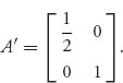
2. Suppose that II plays Y = (y, 1 − y). Then
![]()
There are only two lines to consider in a graph for the game and these two lines intersect at ![]() y = 1 − y, so that y* =
y = 1 − y, so that y* = ![]() . The optimal strategy for II is Y* = (
. The optimal strategy for II is Y* = (![]() ,
, ![]() ), so II should call two-thirds of the time and fold one-third of the time (assuming I bets). The value of the game is then at the point of intersection v =
), so II should call two-thirds of the time and fold one-third of the time (assuming I bets). The value of the game is then at the point of intersection v = ![]() . Note that when there are only two lines, there is no need to actually draw the graph because we know that the optimal point must be at the point of intersection of the two lines, and no other lines are involved.
. Note that when there are only two lines, there is no need to actually draw the graph because we know that the optimal point must be at the point of intersection of the two lines, and no other lines are involved.
3. For player I, suppose that he plays X = (x, 1 − x). Then
![]()
Since there are only two lines, we again calculate the intersection point and obtain the optimal strategy for I as X* = (0, 0, ![]() ,
, ![]() ).
).
Player II is at a distinct disadvantage since the value of this game is v = ![]() . Player II in fact would never be induced to play the game unless player I pays II exactly
. Player II in fact would never be induced to play the game unless player I pays II exactly ![]() before the game begins. That would make the value zero and hence a fair game.
before the game begins. That would make the value zero and hence a fair game.
Now we see a very interesting phenomenon that is well known to poker players. Namely, the optimal strategy for player I has him betting one-third of the time when he has a losing card (king). We expected some type of result like this because of the incentive for player I to bet even when he has a king. So bluffing with positive probability is a part of an optimal strategy when done in the right proportion.
Problems
1.27 In the 2 × 2 Nim game, we saw that v+= v− = − 1. Reduce the game matrix using dominance.
1.28 Consider the matrix game

1.29 Use the methods of this section to solve the games
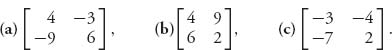
1.30 Use (convex) dominance and the graphical method to solve the game with matrix
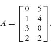
1.31 The third column of the matrix
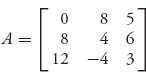
is dominated by a convex combination. Reduce the matrix and solve the game.
1.32 Four army divisions attack a town along two possible roads. The town has three divisions defending it. A defending division is dug in and hence equivalent to two attacking divisions. Even one division attacking an undefended road captures the town. Each commander must decide how many divisions to attack or defend each road. If the attacking commander captures a road to the town, the town falls. Score 1 to the attacker if the town falls and −1 if it doesn’t.
1.33 Consider the matrix game 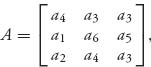 where a1 < a2 < ... < a5 < a6. Use dominance to solve the game.
1.34 Aggie and Baggie are fighting a duel each with one lemon meringue pie starting at 20 paces. They can each choose to throw the pie at either 20 paces, 10 paces, or 0 paces. The probability either player hits the other at 20 paces is ![]() at 10 paces it is
at 10 paces it is ![]() and at 0 paces it is 1. If they both hit or both miss at the same number of paces, the game is a draw. If a player gets a pie in the face, the score is −1, the player throwing the pie gets +1.
and at 0 paces it is 1. If they both hit or both miss at the same number of paces, the game is a draw. If a player gets a pie in the face, the score is −1, the player throwing the pie gets +1.
Set this up as a matrix game and solve it.
1.35 Consider the game with matrix
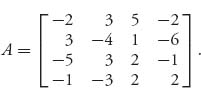
Someone claims that the strategies X* = ![]() , 0,
, 0, ![]() , 0) and
, 0) and ![]() are optimal.
are optimal.
1.36 In the baseball game Example 1.8, it turns out that an optimal strategy for player I, the batter, is given by ![]() and the value of the game is
and the value of the game is ![]() . It is amazing that the batter should never expect a curveball with these payoffs under this optimal strategy. What is the pitcher’s optimal strategy Y*?
. It is amazing that the batter should never expect a curveball with these payoffs under this optimal strategy. What is the pitcher’s optimal strategy Y*?
1.37 In a football game, we use the matrix ![]() The offense is the row player. The first row is Run, the second is Pass. The first column is Defend against Run, the second is Defend against the Pass.
The offense is the row player. The first row is Run, the second is Pass. The first column is Defend against Run, the second is Defend against the Pass.
1.38 Two players Reinhard and Carla play a number game. Carla writes down a number 1, 2, or 3. Reinhard chooses a number (again 1, 2, or 3) and guesses that Carla has written down that number. If Reinhard guesses right he wins $1 from Carla; if he guesses wrong, Carla tells him if his number is higher or lower and he gets to guess again. If he is right, no money changes hands but if he guesses wrong he pays Carla $1.
![]()
1.39 We have an infinite sequence of numbers 0 < a1 ≤ a2 ≤ a3 ≤ .. . Each of two players chooses an integer independent of the other player. If they both happen to choose the same number k, then player I receives ak dollars from player II. Otherwise, no money changes hand. Assume that ![]()
1.40 Show that for any strategy X = (x1, ..., xn) ![]() Sn and any numbers b1, ..., bn, it must be that
Sn and any numbers b1, ..., bn, it must be that
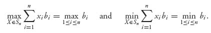
1.41 The properties of optimal strategies (Section 1.3.1) show that X* ![]() Sn and Y*
Sn and Y* ![]() Sm are optimal if and only if minj E(X*, j) = maxi E(i, Y*). The common value will be the value of the game. Verify this.
Sm are optimal if and only if minj E(X*, j) = maxi E(i, Y*). The common value will be the value of the game. Verify this.
1.42 Show that if (X*, Y*) and (X0, Y0) are both saddle points for the game with matrix A, then so is (X*, Y0) and (X0, Y*). In fact, show that (Xλ, Yβ) where X λ = λ X* + (1-λ)X0, Yβ = β Y* + (1 − β)Y0 and λ, β any numbers in [0, 1], is also a saddle point. Thus if there are two saddle points, there are an infinite number.
1.6 Best Response Strategies
If you are playing a game and you determine, in one way or another, that your opponent is using a particular strategy, or is assumed to use a particular strategy, then what should you do? To be specific, suppose that you are player I and you know, or simply assume, that player II is using the mixed strategy Y, optimal or not for player II. In this case you should play the mixed strategy X that maximizes E(X, Y). This strategy that you use would be a best response to the use of Y by player II. The best response strategy to Y may not be the same as what you would use if you knew that player II were playing optimally; that is, it may not be a part of a saddle point. Here is the precise definition.
Definition 1.6.1 A mixed strategy X* for player I is a best response strategy to the strategy Y for player II if it satisfies
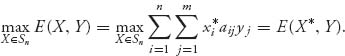
A mixed strategy Y* for player II is a best response strategy to the strategy X for player I if it satisfies
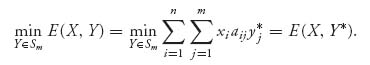
Incidentally, if (X*, Y*) is a saddle point of the game, then X* is the best response to Y*, and vice versa. Unfortunately, knowing this doesn’t provide a good way to calculate X* and Y* because they are both unknown at the start.
Example 1.19 Consider the 3 × 3 game
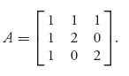
The saddle point is X* = (0, ![]() ,
, ![]() ) = Y* and v(A) = 1. Now suppose that player II, for some reason, thinks she can do better by playing Y = (
) = Y* and v(A) = 1. Now suppose that player II, for some reason, thinks she can do better by playing Y = (![]() ,
, ![]() ,
, ![]() ). What is an optimal response strategy for player I?
). What is an optimal response strategy for player I?
Let X = (x1, x2, 1 − x1 − x2). Calculate
![]()
We want to maximize this as a function of x1, x2 with the constraints 0 ≤ x1, x2 ≤ 1. We see right away that E(X, Y) is maximized by taking x1 = x2 = 0 and then necessarily x3 = 1. Hence, the best response strategy for player I if player II uses Y = (![]() ,
, ![]() ,
, ![]() ) is X* = (0, 0, 1). Then, using this strategy, the expected payoff to I is E(X*, Y) =
) is X* = (0, 0, 1). Then, using this strategy, the expected payoff to I is E(X*, Y) = ![]() , which is larger than the value of the game v(A) = 1. So that is how player I should play if player II decides to deviate from the optimal Y. This shows that any deviation from a saddle could result in a better payoff for the opposing player. However, if one player knows that the other player will not use her part of the saddle, then the best response may not be the strategy used in the saddle. In other words, if (X*, Y*) is a saddle point, the best response to Y ≠ Y* may not be X*, but some other X, even though it will be the case that E(X*, Y) ≥ E(X*, Y*).
, which is larger than the value of the game v(A) = 1. So that is how player I should play if player II decides to deviate from the optimal Y. This shows that any deviation from a saddle could result in a better payoff for the opposing player. However, if one player knows that the other player will not use her part of the saddle, then the best response may not be the strategy used in the saddle. In other words, if (X*, Y*) is a saddle point, the best response to Y ≠ Y* may not be X*, but some other X, even though it will be the case that E(X*, Y) ≥ E(X*, Y*).
Because E(X, Y) is linear in each strategy when the other strategy is fixed, the best response strategy for player I will usually be a pure strategy. For instance, if Y is given, then E(X, Y) = a x1 + b x2 + c x3, for some values a, b, c that will depend on Y and the matrix. The maximum payoff is then achieved by looking at the largest of a, b, c, and taking xi = 1 for the x multiplying the largest of a, b, c, and the remaining values of xj = 0. How do we know that? Well, to show you what to do in general, we will show that
(1.4)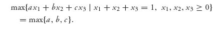
Suppose that max{a, b, c} = c for definiteness. Now, by taking x1 = 0, x2 = 0, x3=1, we get
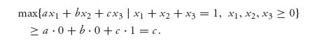
On the other hand, since x1 + x2 + x3 = 1, we see that
![]()
since a − c >0, b − c > 0, and x1, x2 ≥ 0. So, we conclude that
![]()
and this establishes (1.4). This shows that X* = (0, 0, 1) is a best response to Y.
It is possible to get a mixed strategy best response but only if some or all of the coefficients a, b, c are equal. For instance, if b = c, then
![]()
To see this, suppose that max{a, c} = c. We compute
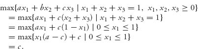
This maximum is achieved at X* = (0, x2, x3) for any x2+ x3=1, x2 ≥ 0, x3 ≥ 0, and we see that we can get a mixed strategy as a best response.
In general, if one of the strategies, say, Yis given and known, then
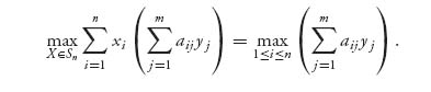
In other words,
![]()
We proved this in the proof of Theorem 1.3.8, part (e).
Best response strategies are frequently used when we assume that the opposing player is Nature or some nebulous player that we think may be trying to oppose us, like the market in an investment game, or the weather. The next example helps to make this more precise.
Example 1.20 Suppose that player I has some money to invest with three options: stock (S), bonds (B), or CDs (certificates of deposit). The rate of return depends on the state of the market for each of these investments. Stock is considered risky, bonds have less risk than stock, and CDs are riskless. The market can be in one of three states: good (G), neutral (N), or bad (B), depending on factors such as the direction of interest rates, the state of the economy, prospects for future growth. Here is a possible game matrix in which the numbers represent the annual rate of return to the investor who is the row player:
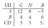
The column player is the market. This game does not have a saddle in pure strategies. (Why?) If player I assumes that the market is the opponent with the goal of minimizing the investor’s rate of return, then we may look at this as a two-person zero sum game. On the other hand, if the investor thinks that the market may be in any one of the three states with equal likelihood, then the market will play the strategy Y = (![]() ,
, ![]() ,
, ![]() ), and then the investor must choose how to respond to that; that is, the investor seeks an X* for which E(X*, Y) = maxX
), and then the investor must choose how to respond to that; that is, the investor seeks an X* for which E(X*, Y) = maxX ![]() S3 E(X, Y), where Y = (
S3 E(X, Y), where Y = (![]() ,
, ![]() ,
, ![]() ). Of course, the investor uses the same procedure no matter which Y she thinks the market will use. The investor can use this game to compare what will happen under various Y strategies.
). Of course, the investor uses the same procedure no matter which Y she thinks the market will use. The investor can use this game to compare what will happen under various Y strategies.
This problem may actually be solved fairly easily. If we assume that the market is an opponent in a game then the value of the game is v(A) = 5, and there are many optimal strategies, one of which is X* = (0, 0, 1), Y* = (0, ![]() ,
, ![]() ). If instead Y = (
). If instead Y = (![]() ,
, ![]() ,
, ![]() ), then the best response for player I is X = (0, 0, 1), with payoff to I equal to 5. If Y = (
), then the best response for player I is X = (0, 0, 1), with payoff to I equal to 5. If Y = (![]() , 0,
, 0, ![]() ), the best response is X = (1, 0, 0), that is, invest in the stock if there is a
), the best response is X = (1, 0, 0), that is, invest in the stock if there is a ![]() probability of a good market. The payoff then is
probability of a good market. The payoff then is ![]() > 5.
> 5.
It may seem odd that the best response strategy in a zero sum two-person game is usually a pure strategy, but it can be explained easily with a simple example. Suppose that someone is flipping a coin that is not fair—say heads comes up 75% of the time. On each toss you have to guess whether it will come up heads or tails. How often should you announce heads in order to maximize the percentage of time you guess correctly? If you think it is 75% of the time, then you will be correct 75 × 75 = 56.25 of the time! If you say heads all the time, you will be correct 75% of the time, and that is the best you can do.
Here is a simple game with an application of game theory to theology!
Example 1.21 Blaise Pascal constructed a game to show that belief in God is the only rational strategy. The model assumes that you are player I, and you have two possible strategies: believe or don’t believe. The opponent is taken to be God, who either plays God exists, or God doesn’t exist. (Remember, God can do anything without contradiction.) Here is the matrix, assuming α, β, γ > 0:
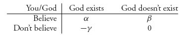
If you believe and God doesn’t exist, then you receive −β because you have foregone evil pleasures in the belief God exists. If you don’t believe and God exists, then you pay a price −γ. Pascal argued that this would be a big price. If you believe and God exists, then you receive the amount α, from God, and Pascal argued this would be a very large amount of spiritual currency.
To solve the game, we first calculate v+ and v− . Clearly v+ = 0 and v− = (−β, −γ) > 0, so this game does not have a saddle point in pure strategies unless β = 0 or γ = 0. If there is no loss or gain to you if you play don’t believe, then that is what you should do, and God should play not exist. In this case, the value of the game is zero.
Assuming that none of α, β, or γ is zero, we will have a mixed strategy saddle. Let Y = (y, 1 − y)be an optimal strategy for God. Then it must be true that
![]()
These are the two equations for a mixed strategy from the graphical method. Solving, we get that y = β/(α + β + γ). The optimal strategy for God is
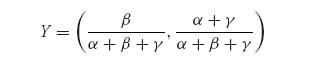
and the value of the game to you is
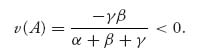
Your optimal strategy X = (x, 1 − x) must satisfy
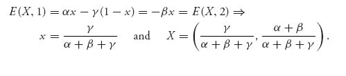
Pascal argued that if γ, the penalty to you if you don’t believe and God exists is loss of eternal life, represented by a very large number. In this case, the percent of time you play believe, x = γ/(α + β + γ) should be fairly close to 1, so you should play believe with high probability. For example, if α = 10, β = 5, γ = 100, then x = 0.87.
From God’s point of view, if γ is a very large number and this is a zero sum game, God would then play doesn’t exist with high probability!! It may not make much sense to think of this as a zero sum game, at least not theologically. Maybe we should just look at this like a best response for you, rather than as a zero sum game.
So, let’s suppose that God plays the strategy Y0= (![]() ,
, ![]() ). What this really means is that you think that God’s existence is as likely as not. What is your best response strategy? For that, we calculate f (x) = E(X, Y0), where X = (x, 1 − x), 0 ≤ x ≤ 1. We get
). What this really means is that you think that God’s existence is as likely as not. What is your best response strategy? For that, we calculate f (x) = E(X, Y0), where X = (x, 1 − x), 0 ≤ x ≤ 1. We get
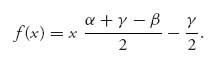
The maximum of f(x) over X ![]() [0, 1]is
[0, 1]is
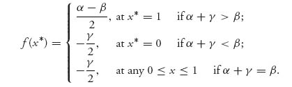
Pascal argued that γ would be a very large number (and so would α) compared to β . Consequently, the best response strategy to Y0 would be X* = (1, 0). Any rational person who thinks that God’s existence is as likely as not would choose to play believe.
Are we really in a zero sum game with God? Probably not because it is unlikely that God loses if you choose to believe. A more likely opponent in a zero sum game like this might be Satan. Maybe the theological game is nonzero sum so that both players can win (and both can lose). In any case, a nonzero sum model of belief will be considered later.
Problems
1.43 Consider the game with matrix
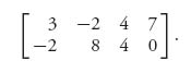
1.44 An entrepreneur, named Victor, outside Laguna beach can sell 500 umbrellas when it rains and 100 when the sun is out along with 1000 pairs of sunglasses. Umbrellas cost him $5 each and sell for $10. Sunglasses wholesale for 2$ and sell for $5. The vendor has $2500 to buy the goods. Whatever he doesn’t sell is lost as worthless at the end of the day.
1.45 You’re in a bar and a stranger comes to you with a new pickup strategy.10 The stranger proposes that you each call Heads or Tails. If you both call Heads, the stranger pays you $3. If both call Tails, the stranger pays you $1. If the calls aren’t a match, then you pay the stranger $2.
1.46 Suppose that the batter in the baseball game Example 1.8 hasn’t done his homework to learn the percentages in the game matrix. So, he uses the strategy X* = (![]() ,
, ![]() ,
, ![]() ). What is the pitcher’s best response strategy?
). What is the pitcher’s best response strategy?
1.47 In general, if we have two payoff functions f(x, y) for player I and g(x, y) for player II, suppose that both players want to maximize their own payoff functions with the variables that they control. Then y* =y*(x) is a best response of player II to x if
![]()
and x* =x*(y) is a best response of player I to y if
![]()
1.6.1 MAPLETM/MATHEMATICA®
1. Find the upper and lower values of a matrix game. Let’s consider the matrix
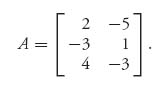
A simple calculation shows that v− = − 3 and v+ = 1. Here are the Maple commands to get this. These commands would be useful mostly for games with large matrices.
> with(LinearAlgebra):
> A:=Matrix([[2, -5], [-3, 1], [4, -3]]);
> rows:=3: cols:=2:
> vu:=min(seq(max(seq(A[i, j], i = 1..rows)), j = 1..cols));
> vl:=max(seq(min(seq(A[i, j], j = 1..cols)), i = 1..rows));
> print("the upper value is", vu);
> print("the lower value is", vl);
The number of rows and column could be obtained from Maple by using the statement rows:=RowDimension(A); cols:=ColumnDimension(A).
Incidentally, two very simple Maple commands gives the solution of the system of equations very quickly. Here they are:
> eqs:={y1+2*y2+3*y3-v = 0,
 3*y1+y2+2*y3-v = 0,
 2*y1+3*y2+y3-v = 0,
 y1+y2+y3-1 = 0};
> solve(eqs, [y1, y2, y3, v]);
Maple gives us the same solution we got by hand.
Bibliographic Notes
The classic reference for the material in this chapter is the wonderful two-volume set of books by Karlin11 (1992), one of the pioneers of game theory when he was a member of the Rand Institute. The proofs of the von Neumann minimax theorem are modifications of those in Karlin’s book. Proof 2, which uses only advanced calculus, is original to Karlin. On the other hand, the birth of game theory can be dated to the appearance of the seminal book by von Neumann and Morgenstern, (1953).
The idea of using mixed strategies in order to establish the existence of a saddle point in this wider class is called relaxation. This idea is due to von Neumann and extends to games with continuous strategies, as well as the modern theory of optimal control, differential games, and the calculus of variations. It has turned out to be one of the most far-reaching ideas of the twentieth century.
The graphical solution of matrix games is extremely instructive as to the objectives for each player. Apparently, this method is present at the founding of game theory, but its origin is unknown to the author of this book.
The Russian roulette Example 1.5 is an adaptation of a similar example in the book by Jones (2000). Poker models have been considered from the birth of game theory. Any gambler interested in poker should consult the book by Karlin (1992) for much more information and results on poker models.
The ideas of a best response strategy and viewing a saddle point as a pair of strategies, each of which is a best response to the other, leads naturally in later chapters to a Nash equilibrium for more general games.
1 Referred to neutrally as he, she, or player.
2 The numbers in this matrix would be gathered by a statistical analysis of the history of this batter with this pitcher.
3 The interested reader can see the book Winning Ways for Your Mathematical Plays (Academic Press, 1982) by Elwyn R. Berlekamp, John H. Conway, and Richard K. Guy.
4 If X is a random variable taking values x1, x2, ..., xn with probabilities p1, p_2, ..., pn, respectively, then EX = ![]() i = 1n xipi. See the Appendix B for more details.
i = 1n xipi. See the Appendix B for more details.
5 The proof may be skipped but there are some exercises for this section that may be instructive.
6 These proofs follow the presentation by Karlin (1992).
7 That is, for any sequences xn ![]() C, y_n
C, y_n ![]() g(xn), if xn → x and yn → y, then y
g(xn), if xn → x and yn → y, then y ![]() g(x).
g(x).
8 This is a statement in probability theory called the Law of Large Numbers.
9 This will introduce us to information sets for extensive games. The nodes at B and B for player II should be connected as an information set for player II. Player II knows that I has Bet, but she doesn’t know which branch the B came from.
10 This question appeared in a column by Marilyn Vos Savant in Parade Magazine on March 31, 2002.
11 June 8, 1924 – December 18, 2007, was Professor of Mathematics and Statistics at Stanford University from 1956 to his death.