
CHAPTER THREE
Two-Person Nonzero Sum Games
But war’s a game, which, were their subjects wise, Kings would not play at.
—William Cowper, The Winter Morning Walk
I made a game effort to argue but two things were against me: the umpires and the rules.
—Leo Durocher
All things are subject to interpretation. Whichever interpretation prevails at a given time is a function of power and not truth.
—Friedrich Nietzsche
If past history was all there was to the game, the richest people would be librarians.
—Warren Buffett
3.1 The Basics
The previous chapter considered two-person games in which whatever one player gains, the other loses. This is far too restrictive for many games, especially games in economics or politics, where both players can win something or both players can lose something. We no longer assume that the game is zero sum, or even constant sum. All players will have their own individual payoff matrix and the goal of maximizing their own individual payoff. We will have to reconsider what we mean by a solution, how to get optimal strategies, and exactly what is a strategy.
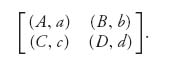
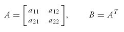
In a two-person nonzero sum game, we simply assume that each player has her or his own payoff matrix. Suppose that the payoff matrices are as follows:
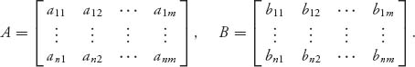
For example, if player I plays row 1 and player II plays column 2, then the payoff to player I is a12 and the payoff to player II is b12. In a zero sum game, we always had aij + bij = 0, or more generally aij + bij= k, where k is a fixed constant. In a nonzero sum game, we do not assume that. Instead, the payoff when player I plays row i and player II plays column j is now a pair of numbers (aij, bij) where the first component is the payoff to player I and the second number is the payoff to player II. The individual rows and columns are called pure strategies for the players. Finally, every zero sum game can be put into the bimatrix framework by taking B = −A, so this is a true generalization of the theory in the first chapter. Let’s start with a simple example.
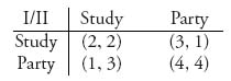
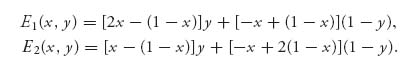
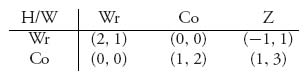
Example 3.1 Two students have an exam tomorrow. They can choose to study, or go to a party. The payoff matrices, written together as a bimatrix, are given by
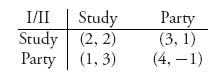
If they both study, they each receive a payoff of 2, perhaps in grade point average points. If player I studies and player II parties, then player I receives a better grade because the curve is lower. But player II also receives a payoff from going to the party (in good time units). If they both go to the party, player I has a really good time, but player II flunks the exam the next day and his girlfriend is stolen by player I, so his payoff is −1 What should they do?
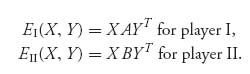
Players can choose to play pure strategies, but we know that greatly limits their options. If we expect optimal strategies to exist Chapters 1 and 2 have shown we must allow mixed strategies. A mixed strategy for player I is again a vector (or matrix) X = (x1, …, xn) ![]() Sn with xi ≥ 0 representing the probability that player I uses row i, and x1 + x2 + … + xn = 1. Similarly, a mixed strategy for player II is Y = (y1, …, ym)
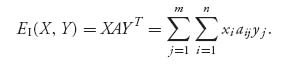
Sn with xi ≥ 0 representing the probability that player I uses row i, and x1 + x2 + … + xn = 1. Similarly, a mixed strategy for player II is Y = (y1, …, ym) ![]() Sm, with yj ≥ 0 and y1 + … + ym = 1. Now given the player’s choice of mixed strategies, each player will have their own expected payoffs given by
Sm, with yj ≥ 0 and y1 + … + ym = 1. Now given the player’s choice of mixed strategies, each player will have their own expected payoffs given by
We need to define a concept of optimal play that should reduce to a saddle point in mixed strategies in the case B = −A. It is a fundamental and far-reaching definition due to another genius of mathematics who turned his attention to game theory in the middle twentieth century, John Nash1.
Definition 3.1.1 A pair of mixed strategies (X* ![]() Sn, Y*
Sn, Y* ![]() Sm) is a Nash equilibrium if EI(X, Y*) ≤ EI(X*, Y*) for every mixed X
Sm) is a Nash equilibrium if EI(X, Y*) ≤ EI(X*, Y*) for every mixed X ![]() Sn and EII(X*, Y) ≤ EII(X*, Y*) for every mixed Y
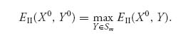
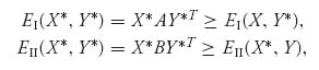
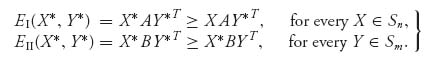
Sn and EII(X*, Y) ≤ EII(X*, Y*) for every mixed Y ![]() Sm. If (X*, Y*) is a Nash equilibrium we denote by vA = EI(X*, Y*) and vB = EII(X*, Y*) as the optimal payoff to each player. Written out with the matrices, (X*, Y*) is a Nash equilibrium if
Sm. If (X*, Y*) is a Nash equilibrium we denote by vA = EI(X*, Y*) and vB = EII(X*, Y*) as the optimal payoff to each player. Written out with the matrices, (X*, Y*) is a Nash equilibrium if
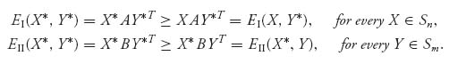
This says that neither player can gain any expected payoff if either one chooses to deviate from playing the Nash equilibrium, assuming that the other player is implementing his or her piece of the Nash equilibrium. On the other hand, if it is known that one player will not be using his piece of the Nash equilibrium, then the other player may be able to increase her payoff by using some strategy other than that in the Nash equilibrium. The player then uses a best response strategy. In fact, the definition of a Nash equilibrium says that each strategy in a Nash equilibrium is a best response strategy against the opponent’s Nash strategy. Here is a precise definition for two players.
Definition 3.1.2 A strategy X0 ![]() Sn is a best response strategy to a given strategy Y0
Sn is a best response strategy to a given strategy Y0 ![]() Sm for player II, if
Sm for player II, if
![]()
Similarly, a strategy Y0 ![]() Sm is a best response strategy to a given strategy X0
Sm is a best response strategy to a given strategy X0 ![]() Sn for player I, if
Sn for player I, if
In particular, another way to define a Nash equilibrium (X*, Y*) is that X* maximizes EI(X, Y*) over all X ![]() Sn and Y* maximizes EII(X*, Y) over all Y
Sn and Y* maximizes EII(X*, Y) over all Y ![]() Sm. X* is a best response to Y* and Y* is a best response to X*.
Sm. X* is a best response to Y* and Y* is a best response to X*.
Remark It is important to note what a Nash equilibrium is not. A Nash equilibrium does not maximize the payoff to each player. That would make the problem trivial because it would simply say that the Nash equilibrium is found by maximizing a function (the first player’s payoff) of two variables over both variables, and then requiring that it also maximize the second player’s payoff at the same point. That would be a rare occurrence but trivial from a mathematical point of view to find (if one existed).
If B = −A, a bimatrix game is a zero sum two-person game and a Nash equilibrium is the same as a saddle point in mixed strategies. It is easy to check that from the definitions because EI(X, Y) = X AYT = − EII(X, Yx).
Note that a Nash equilibrium in pure strategies will be a row i* and column j* satisfying

So ai* j* is the largest number in column j* and bi* j* is the largest number in row i*. In the bimatrix game, a Nash equilibrium in pure strategies must be the pair that is, at the same time, the largest first component in the column and the largest second component in the row.
Just as in the zero sum case, a pure strategy can always be considered as a mixed strategy by concentrating all the probability at the row or column, which should always be played.
As in earlier sections, we will use the notation that if player I uses the pure strategy row i, and player II uses mixed strategy Y ![]() Sm, then the expected payoffs to each player are
Sm, then the expected payoffs to each player are
![]()
Similarly, if player II uses column j and player I uses the mixed strategy X, then
![]()
The questions we ask for a given bimatrix game are as follows:
To start, we consider the classic example.
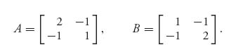
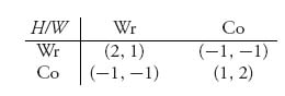
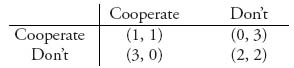
Prisoner’s Dilemma. Two criminals have just been caught after committing a crime. The police interrogate the prisoners by placing them in separate rooms so that they cannot communicate and coordinate their stories. The goal of the police is to try to get one or both of them to confess to having committed the crime. We consider the two prisoners as the players in a game in which they have two pure strategies: confess, or don’t confess. Their prison sentences, if any, will depend on whether they confess and agree to testify against each other. But if they both confess, no benefit will be gained by testimony that is no longer needed. If neither confesses, there may not be enough evidence to convict either of them of the crime. The following matrices represent the possible payoffs remembering that they are set up to maximize the payoff:
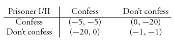
The individual matrices for the two prisoners are as follows:
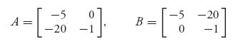
The numbers are negative because they represent the number of years in a prison sentence and each player wants to maximize the payoff, that is, minimize their own sentences.
To see whether there is a Nash equilibrium in pure strategies we are looking for a payoff pair (a, b) in which a is the largest number in a column and b is the largest number in a row simultaneously. There may be more than one such pair. Looking at the bimatrix is the easiest way to find them. The systematic way is to put a bar over the first number that is the largest in each column and put a bar over the second number that is the largest in each row. Any pair of numbers that both have bars is a Nash equilibrium in pure strategies. In the prisoner’s dilemma problem, we have
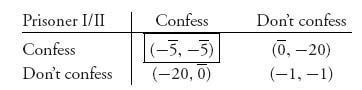
We see that there is exactly one pure Nash equilibrium at (confess, confess), they should both confess and settle for 5 years in prison each. If either player deviates from confess, while the other player still plays confess, then the payoff to the player who deviates goes from −5 to −20.
Wait a minute: clearly both players can do better if they both choose don’t confess because then there is not enough evidence to put them in jail for more than one year. But there is an incentive for each player to not play don’t confess. If one player chooses don’t confess and the other chooses confess, the payoff to the confessing player is 0—he won’t go to jail at all! The players are rewarded for a betrayal of the other prisoner, and so that is exactly what will happen. This reveals a major reason why conspiracies almost always fail. As soon as one member of the conspiracy senses an advantage by confessing, that is exactly what they will do, and then the game is over.
The payoff pair (−1, −1) is unstable in the sense that a player can do better by deviating, assuming that the other player does not, whereas the payoff pair (−5, −5) is stable because neither player can improve their own individual payoff if they both play it. Even if they agree before they are caught to not confess, it would take extraordinary will power for both players to stick with that agreement in the face of the numbers. In this sense, the Nash equilibrium is self-enforcing.
Any bimatrix game in which the Nash equilibrium gives both players a lower payoff than if they cooperated is a prisoner’s dilemma game. In a Prisoner’s dilemma game, the players will choose to not cooperate. That is pretty pessimistic and could lead to lots of bad things which could, but don’t usually happen in the real world. Why not? One explanation is that many such games are not played just once but repeatedly over long periods of time (like arms control, for example). Then the players need to take into account the costs of not cooperating. The conclusion is that a game which is repeated many times may not exhibit the same features as a game played once.
Note that in matrix A in the prisoner’s dilemma, the first row is always better than the second row for player I. This says that for player I, row 1, (i.e., confess), strictly dominates row 2 and hence row 2 can be eliminated from consideration by player I, no matter what player II does because player I will never play row 2. Similarly, in matrix B for the other player, column 1 strictly dominates column 2, so player II, who chooses the columns, would never play column 2. Once again, player II would always confess. This problem can be solved by domination.
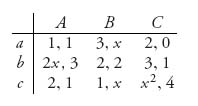
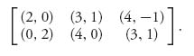
Example 3.2 This example explains what is going on when you are looking for the pure Nash equilibria. Let’s look at the game with matrix
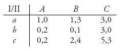
Consider player II:
Now consider player I:
The only pair which is a best response to a best response is If II plays B, then I plays c; If I plays c, then II plays B. It is the only pair (x, y) = (2, 4) with x the largest first number in all the rows and y is the largest second number of all the columns, simultaneously.
Example 3.3 Can a bimatrix game have more than one Nash equilibrium? Absolutely. If we go back to the study–party game and change one number, we will see that it has two Nash equilibria:
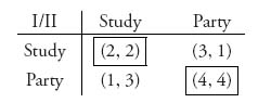
There is a Nash equilibrium at payoff (2, 2) and at (4, 4). Which one is better? In this example, since both students get a payoff of 4 by going to the party, that Nash point is clearly better for both. But if player I decides to study instead, then what is best for player II? That is not so obvious.
In the next example, we get an insight into why countries want to have nuclear bombs.
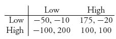
Example 3.4 The Arms Race. Suppose that two countries have the choice of developing or not developing nuclear weapons. There is a cost of the development of the weapons in the price that the country might have to pay in sanctions, and so forth. But there is also a benefit in having nuclear weapons in prestige, defense, deterrence, and so on. Of course, the benefits of nuclear weapons disappear if a country is actually going to use the weapons. If one considers the outcome of attacking an enemy country with nuclear weapons and the risk of having your own country vaporized in retaliation, a rational person would certainly consider the cold war acronym MAD, mutually assured destruction, as completely accurate.
Suppose that we quantify the game using a bimatrix in which each player wants to maximize the payoff:
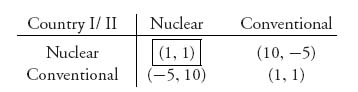
To explain these numbers, if country I goes nuclear and country II does not, then country I can dictate terms to country II to some extent because a war with I, who holds nuclear weapons and will credibly use them, would result in destruction of country II, which has only conventional weapons. The result is a representative payoff of 10 to country I and −5 to country II, as I’s lackey now. On the other hand, if both countries go nuclear, neither country has an advantage or can dictate terms to the other because war would result in mutual destruction, assuming that the weapons are actually used. Consequently, there is only a minor benefit to both countries going nuclear, represented by a payoff of 1 to each. That is the same as if they remain conventional because then they do not have to spend money to develop the bomb, dispose of nuclear waste, and so on.
We see from the bimatrix that we have a Nash equilibrium at the pair (1, 1) corresponding to the strategy (nuclear, nuclear). The pair (1, 1) when both countries maintain conventional weapons is not a Nash equilibrium because each player can improve its own payoff by unilaterally deviating from this. Observe, too, that if one country decides to go nuclear, the other country clearly has no choice but to do likewise. The only way that the situation could change would be to reduce the benefits of going nuclear, perhaps by third-party sanctions or in other ways.
This simple matrix game captures the theoretical basis of the MAD policy of the United States and the former Soviet Union during the cold war. Once the United States possessed nuclear weapons, the payoff matrix showed the Soviet Union that it was in their best interest to also own them and to match the US nuclear arsenal to maintain the MAD option.
Since World War II, the nuclear nonproliferation treaty has attempted to have the parties reach an agreement that they would not obtain nuclear weapons, in other words to agree to play (conventional, conventional). Countries which have instead played Nuclear include India, Pakistan, North Korea, and Israel2 . Iran is playing Nuclear covertly, and Libya, which once played Nuclear, switched to conventional because its payoff changed.
The lesson to learn here is that once one government obtains nuclear weapons, it is a Nash equilibrium—and self-enforcing equilibrium—for opposing countries to also obtain the weapons.
Example 3.5 Do all bimatrix games have Nash equilibrium points in pure strategies? Game theory would be pretty boring if that were true. For example, if we look at the game
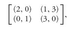
there is no pair (a, b) in which a is the largest in the column and b is the largest in the row. In a case like this, it seems reasonable that we use mixed strategies. In addition, even though a game might have pure strategy Nash equilibria, it could also have a mixed strategy Nash equilibrium.
In the next section, we will see how to solve such games and find the mixed Nash equilibria.
Finally, we end this section with a concept that is a starting point for solving bimatrix games and that we will use extensively when we discuss cooperation. Each player asks, what is the worst that can happen to me in this game?
The amount that player I can be guaranteed to receive is obtained by assuming that player II is actually trying to minimize player I’s payoff. In the bimatrix game with two players with matrices (An × m, Bn × m), we consider separately the two games arising from each matrix. Matrix A is considered as the matrix for a zero sum game with player I against player II (player I is the row player=maximizer and player II is the column player=minimizer). The value of the game with matrix A is the guaranteed amount for player I. Similarly, the amount that player II can be guaranteed to receive is obtained by assuming player I is actively trying to minimize the amount that II gets. For player II, the zero sum game is BT because the row player is always the maximizer. Consequently, player II can guarantee that she will receive the value of the game with matrix BT. The formal definition is summarized below.
Definition 3.1.3 Consider the bimatrix game with matrices (A, B). The safety value for player I is value(A). The safety value for player II in the bimatrix game is value(BT).
If A has the saddle point (XA, YA), then XA is called the maxmin strategy for player I.
If BT has saddle point (XBT, YBT), then XBT is the maxmin strategy for player II.
In the prisoner’s dilemma game, the safety values are both −5 to each player, as you can quickly verify.
In the game with matrix
we have
Then ![]() is the safety value for player I and
is the safety value for player I and ![]() is the safety value for player II.
is the safety value for player II.
The maxmin strategy for player I is ![]() , and the implementation of this strategy guarantees that player I can get at least her safety level. In other words, if I uses
, and the implementation of this strategy guarantees that player I can get at least her safety level. In other words, if I uses ![]() , then
, then ![]() no matter what Y strategy is used by II. In fact,
no matter what Y strategy is used by II. In fact,
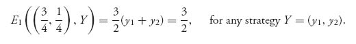
The maxmin strategy for player II is ![]() which she can use to get at least her safety value of
which she can use to get at least her safety value of ![]() .
.
Is there a connection between the safety levels and a Nash equilibrium? The safety levels are the guaranteed amounts each player can get by using their own individual maxmin strategies, so any rational player must get at least the safety level in a bimatrix game. In other words, it has to be true that if (X*, Y*) is a Nash equilibrium for the bimatrix game (A, B), then
![]()
This would say that in the bimatrix game, if players use their Nash points, they get at least their safety levels. That’s what it means to be individually rational. Precisely, two strategies X, Y are individually rational if EI(X, Y) ≥ v(A) and EII(X, Y) ≥ v(BT).
Here’s why any Nash equilibrium is individually rational.
Proof. It is really just from the definitions. The definition of Nash equilibrium says
![]()
But if that is true for all mixed X, then
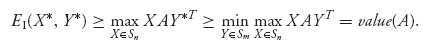
The other part of a Nash definition gives us
Each player does at least as well as assuming the worst. ![]()
Problems
3.1 Show that (X*, Y*) is a saddle point of the game with matrix A if and only if (X*, Y*) is a Nash equilibrium of the bimatrix game (A, −A).
3.2 Suppose that a married couple, both of whom have just finished medical school, now have choices regarding their residencies. One of the new doctors has three choices of programs, while the other has two choices. They value their prospects numerically on the basis of the program itself, the city, staying together, and other factors, and arrive at the bimatrix
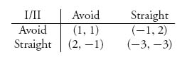
3.3 Consider the bimatrix game that models the game of chicken:
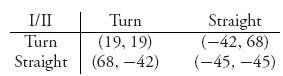
Two cars are headed toward each other at a high rate of speed. Each player has two options: turn off, or continue straight ahead. This game is a macho game for reputation, but leads to mutual destruction if both play straight ahead.
3.4 We may eliminate a row or a column by dominance. If aij ≥ ai′ j for every column j, and we have strict inequality for some column j, then we may eliminate row i′. If player I drops row i′, then the entire pair of numbers in that row are dropped. Similarly, if bij ≥ bij′ for every row i, and we have strict inequality for some row i, then we may drop column j′, and all the pairs of payoffs in that column. If the inequalities are all strict, this is called strict dominance, otherwise it is weak dominance.
3.5 When we have weak dominance in a game, the order of removal of the dominated row or column makes a difference. Consider the matrix
3.6 Suppose two merchants have to choose a location along the straight road. They may choose any point in {1, 2, …, n}. Assume there is exactly one customer at each of these points and a customer will always go to the nearest merchant. If the two merchants are equidistant to a customer then they share that customer, that is, ![]() the customer goes to each store. For example, if n = 11 and if player I chooses location 3 and player II chooses location 8, then the payoff to I is 5 and the payoff to II is 6.
the customer goes to each store. For example, if n = 11 and if player I chooses location 3 and player II chooses location 8, then the payoff to I is 5 and the payoff to II is 6.
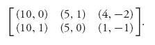
3.7 Two airlines serve the route ORD to LAX. Naturally, they are in competition for passengers who make their decision based on airfares alone. Lower fares attract more passengers and increases the load factor (the number of bodies in seats). Suppose the bimatrix is given as follows where each airline can choose to set the fare at Low = $250 or High = $700:
The numbers are in millions. Find the pure Nash equilibria.
3.8 Consider the game with bimatrix
3.2 2 × 2 Bimatrix Games, Best Response, Equality of Payoffs
Now we will analyze all two-person 2 × 2 nonzero sum games. We are after a method to find all Nash equilibria for a bimatrix game, mixed and pure. Let X = (x, 1 − x), Y = (y, 1 − y), 0 ≤ x ≤ 1, 0 ≤ y ≤ 1 be mixed strategies for players I and II, respectively. As in the zero sum case, X represents the mixture of the rows that player I has to play; specifically, player I plays row 1 with probability x and row 2 with probability 1 − X. Similarly for player II and the mixed strategy Y. Now we may calculate the expected payoff to each player. As usual,
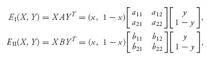
are the expected payoffs to I and II, respectively. It is the goal of each player to maximize her own expected payoff assuming that the other player is doing her best to maximize her own payoff with the strategies she controls.
Let’s proceed to figure out how to find mixed Nash equilibria. First, we need a definition of a certain set.
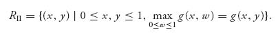
Definition 3.2.1 Let X = (x, 1 − X), Y = (y, 1 − y) be strategies, and set f(x, y) = EI(X, Y), and g(x, y) = EII(X, Y). The rational reaction set for player I is the set of points
![]()
and the rational reaction set for player II is the set
A point (x*, y) ![]() RI means that x* is the point in [0, 1] where x
RI means that x* is the point in [0, 1] where x ![]() f(x, y) is maximized for y fixed. Then X* = (x, 1 − X*) is a best response to Y = (y, 1 − y). Similarly, if (x, y*)
f(x, y) is maximized for y fixed. Then X* = (x, 1 − X*) is a best response to Y = (y, 1 − y). Similarly, if (x, y*) ![]() RII, then y*
RII, then y* ![]() [0, 1] is a point where y
[0, 1] is a point where y ![]() g(x, y) is maximized for x fixed. The strategy Y* = (y*, 1 − y*) is a best response to X = (x, 1 − X). Consequently, a point (x*, y*) in both RI and RII says that X* = (x*, 1 − x*) and Y* = (y*, 1 − y*), as best responses to each other, is a Nash equilibrium.
g(x, y) is maximized for x fixed. The strategy Y* = (y*, 1 − y*) is a best response to X = (x, 1 − X). Consequently, a point (x*, y*) in both RI and RII says that X* = (x*, 1 − x*) and Y* = (y*, 1 − y*), as best responses to each other, is a Nash equilibrium.
3.2.1 CALCULATION OF THE RATIONAL REACTION SETS FOR 2 × 2 GAMES
First, we will show how to find the rational reaction sets for the bimatrix game with matrices (A, B). Let X = (x, 1 − x), Y = (y, 1 − y) be any strategies and define the functions
The idea is to find for a fixed 0 ≤ y ≤ 1, the best response of player I to y; that is, find x ![]() [0, 1] which will give the largest value of player I’s payoff f(x, y) for a given y. Accordingly, we seek
[0, 1] which will give the largest value of player I’s payoff f(x, y) for a given y. Accordingly, we seek
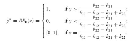
If we use the elements of the matrices we can be more explicit. We know that
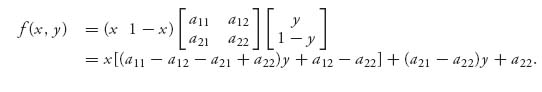
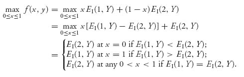
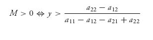
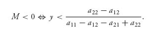
Now we see that in order to make this as large as possible we need only look at the term M = [(a11 − a12 − a21 + a22)y + a12 − a22]. The graph of f for a fixed y is simply a straight line with slope M:
- If M > 0, the maximum of the line will occur at x* = 1.
- If M < 0, the maximum of the line will occur at x* = 0.
- If M = 0, it won’t matter where x is because the line will be horizontal.
Now

and for this given y, the best response is any 0 ≤ x ≤ 1.
If M > 0, the best response to a given y is x* = 1, while if M < 0 the best response is x* = 0. But we know that
and
What we have found is a (set valued) function, called the best response function:
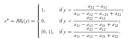
Observe that the best response takes on exactly three values, 0 or 1 or the set [0, 1]. That is not a coincidence because it comes from maximizing a linear function over the interval 0 ≤ x ≤ 1.
The rational reaction set for player I is then the graph of the best response function for player I. In symbols, RI = {(x, y) ![]() [0, 1] × [0, 1] | x = BRI(y)}.
[0, 1] × [0, 1] | x = BRI(y)}.
In a similar way, we may consider the problem for player II. For player II, we seek
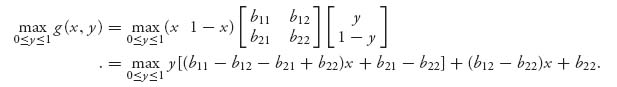
Now we see that in order to make this as large as possible we need only look at the term R = [(b11 − b12 − b21 + b22)x + b21 − b22]. The graph of g for a fixed x is a straight line with slope R:
- If R > 0, the maximum of the line will occur at y* = 1.
- If R < 0, the maximum of the line will occur at y* = 0.
- If R = 0, it won’t matter where y is because the line will be horizontal.
Just as before we derive the best response function for player II:
The rational reaction set for player II is the graph of the best response function for player II. That is, RII = {(x, y) ![]() [0, 1] × [0, 1] | y = BRII(x)} . The points of RI
[0, 1] × [0, 1] | y = BRII(x)} . The points of RI ![]() RII are exactly the (x, y) for which X = (x, 1 − x), Y = (y, 1 − y) are Nash equilibria for the game.
RII are exactly the (x, y) for which X = (x, 1 − x), Y = (y, 1 − y) are Nash equilibria for the game.
Here is a specific example.
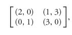
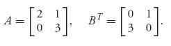
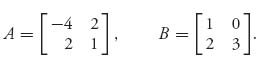
Example 3.6 The bimatrix game with the two matrices
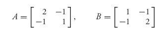
will have multiple Nash equilibria. Two of them are obvious; the pair (2, 1) and the pair (1, 2) in (A, B) have the property that the first number is the largest in the first column and at the same time the second number is the largest in the first row. So we know that X* = (1, 0), Y* = (1, 0) is a Nash point (with payoff 2 for player I and 1 for player II) as is X* = (0, 1), Y* = (0, 1), (with payoff 1 for player I and 2 for player II).
For these matrices
![]()
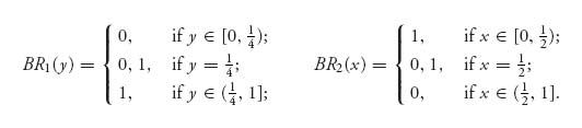
and the maximum occurs at x* which is the best response to a given y ![]() [0, 1], namely,
[0, 1], namely,
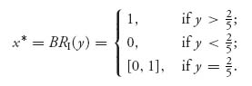
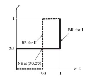
The graph of this is shown in Figure 3.1 below.
Similarly,
![]()
and and the maximum for g when x is given occurs at y*,
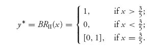
We graph this as the dotted line on the same graph as before (see Figure 3.2).
As you can see the best response functions cross at (x, y) = (0, 0), and (1, 1) on the boundary of the square, but also at ![]() in the interior, corresponding to the unique mixed Nash equilibrium
in the interior, corresponding to the unique mixed Nash equilibrium ![]() . Note that the point of intersection is not a Nash equilibrium, but it gives you the first component of the two strategies that do give the equilibrium. The expected payoffs are as follows:
. Note that the point of intersection is not a Nash equilibrium, but it gives you the first component of the two strategies that do give the equilibrium. The expected payoffs are as follows:
This is curious because the expected payoffs to each player are much less than they could get at the other Nash points.
We will see pictures like Figure 3.2 again in Section 3.3 when we consider an easier way to get Nash equilibria.
FIGURE 3.1 Best response function for player I.
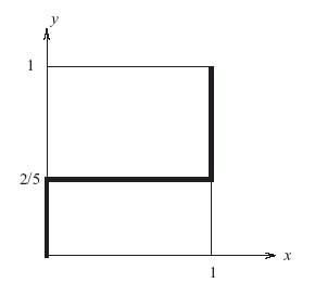
FIGURE 3.2 Best response function for players I and II.
Our next proposition shows that in order to check if strategies (X*, Y*) is a Nash equilibrium, we need only check inequalities in the definition against only pure strategies. This is similar to the result in zero sum games that (X*, Y*) is a saddle and v is the value if and only if E(X*, j) ≥ v and E(i, Y*) ≤ v, for all rows and columns. We will prove it in the 2 × 2 case.
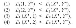
Proposition 3.2.2 (X*, Y*) is a Nash equilibrium if and only if
If the game is 2 × 2, the proposition says
Proposition 3.2.3 A necessary and sufficient condition for X* = (x*, 1 − x*), Y* = (y*, 1 − y*) to be a Nash equilibrium point of the game with matrices (A, B) is
Proof. To see why this is true, we first note that if (X*, Y*) is a Nash equilibrium, then the inequalities must hold by definition (simply choose pure strategies for comparison). We need only to show that the inequalities are sufficient.
Suppose that the inequalities hold for (X*, Y*). Let X = (x, 1 − x) and Y = (y, 1 − y) be any mixed strategies. Successively multiply (1) by x ≥ 0 and (2) by 1 − X ≥ 0 to get
![]()
and
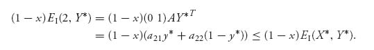
Add these up to get
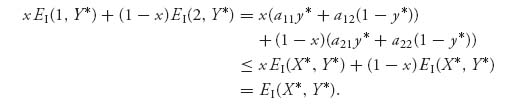
But then, since x EI(1, Y*) + (1 − x)EI(2, Y*) = EI(X, Y*), that is,
![]()
we see that
![]()
Since X ![]() S2 is any old mixed strategy for player I, this gives the first part of the definition that (X*, Y*) is a Nash equilibrium. The rest of the proof is similar and left as an exercise.
S2 is any old mixed strategy for player I, this gives the first part of the definition that (X*, Y*) is a Nash equilibrium. The rest of the proof is similar and left as an exercise. ![]()
One important use of this result is as a check to make sure that we actually have a Nash equilibrium. The next example illustrates that.
Example 3.7 Someone says that the bimatrix game
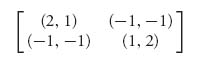
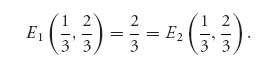
has a Nash equilibrium at ![]() . To check that, first compute EI(X*, Y*) = EII(X*, Y*) =
. To check that, first compute EI(X*, Y*) = EII(X*, Y*) = ![]() . Now check to make sure that this number is at least as good as what could be gained if the other player plays a pure strategy. You can readily verify that, in fact, EI(1, Y*) =
. Now check to make sure that this number is at least as good as what could be gained if the other player plays a pure strategy. You can readily verify that, in fact, EI(1, Y*) = ![]() = EI(2, Y*) and also EII(X*, 1) = EII(X*, 2) =
= EI(2, Y*) and also EII(X*, 1) = EII(X*, 2) = ![]() , so we do indeed have a Nash point.
, so we do indeed have a Nash point.
The most important theorem of this section gives us a way to find a mixed Nash equilibrium of any two-person bimatrix game. It is a necessary condition that may be used for computation and is very similar to the equilibrium theorem for zero sum games. If you recall in Property 3 of (Section 1.3.1) (Proposition 5.1.4), we had the result that in a zero sum game whenever a row, say, row k, is played with positive probability against Y*, then the expected payoff E(k, Y*) must give the value of the game. The next result says the same thing, but now for each of the two players. This is called the equality of payoffs theorem.
Theorem 3.2.4 Equality of Payoffs Theorem. Suppose that
![]()
is a Nash equilibrium for the bimatrix game (A, B).
For any row k that has a positive probability of being used, xk > 0, we have EI(k, Y*) = EI(X*, Y*) ![]() vI.
vI.
For any column j that has a positive probability of being used, yj > 0, we have EII(X*, j) = EII(X*, Y*) ![]() vII (X*, Y*). That is,
vII (X*, Y*). That is,
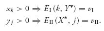
Proof. We know from Proposition 3.2.2 that since we have a Nash point, EI(X*, Y*) = vI ≥ EI(i, Y*) for any row i. Now, suppose that row k has positive probability of being played against Y* and that it gives player I a strictly smaller expected payoff vI > EI(k, Y*). Then vI ≥ EI(i, Y*) for all the rows i = 1, 2, …, n, i ≠ k, and vI > EI(k, Y*) together imply that
![]()
Adding up all these inequalities, we get
This contradiction says it must be true that vI = EI(k, Y*). The only thing that could have gone wrong with this argument is xk = 0. (Why?) Now you can argue in the same way for the assertion about player II. Observe, too, that the argument we just gave is basically the identical one we gave for zero sum games. ![]()
Remark
The idea now is that we can find the (completely) mixed Nash equilibria by solving a system of equations rather than inequalities for player II:
![]()
and
![]()
This won’t be enough to solve the equations, however. You need the additional condition that the components of the strategies must sum to one:
![]()
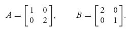
Example 3.8 As a simple example of this theorem, suppose that we take the matrices
Suppose that X = (x1, x2), Y = (y1, y2) is a mixed Nash equilibrium. If 0 < x1 < 1, then, since both rows are played with positive probability, by the equality of payoffs Theorem 3.2.4, vI = EI(1, Y) = EI(2, Y). So the equations
![]()
have solution y1 = 0.143, y2 = 0.857, and then vI = 1.143. Similarly, EII(X, 1) = EII(X, 2) gives
![]()
Note that we can find the Nash point without actually knowing vI or vII. Also, assuming that EI(1, Y) = vI = EI(2, Y) gives us the optimal Nash point for player II, and assuming EII(X, 1) = EII(X, 2) gives us the Nash point for player I. In other words, the Nash point for II is found from the payoff function for player I and vice versa.
Problems
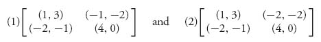
3.9 Suppose we have a two-person matrix game that results in the following best response functions. Find the Nash equilibria if they exist.
3.10 Complete the verification that the inequalities in Proposition 3.2.3 are sufficient for a Nash equilibrium in a 2 × 2 game.
3.11 Apply the method of this section to analyze the modified study–party game:
Find all Nash equilibria and graph the rational reaction sets.
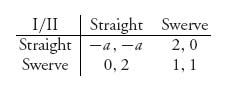
3.12 Consider the Stop–Go game. Two drivers meet at an intersection at the same time. They have the options of stopping and waiting for the other driver to continue, or going.
Here is the payoff matrix in which the player who stops while the other goes loses a bit less than if they both stopped.
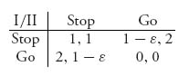
Assume that 0 < ![]() < 1. Find all Nash equilibria.
< 1. Find all Nash equilibria.
3.13 Determine all Nash equilibria and graph the rational reaction sets for the game
3.14 There are two companies each with exactly one job opening. Suppose firm 1 offers the pay p1 and firm 2 offers pay p2 with p1 < p2 < 2p1. There are two prospective applicants each of whom can apply to only one of the two firms. They make simultaneous and independent decisions. If exactly one applicant applies to a company, that applicant gets the job. If both apply to the same company, the firm flips a fair coin to decide who is hired and the other is unemployed (payoff zero).
3.15 This problem looks at the general 2 × 2 game to compute a mixed Nash equilibrium:
3.16 This game is the nonzero sum version of Pascal’s wager (see Example 1.21).
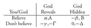
Since God choosing to not exist is paradoxical, we change God’s strategies to Reveals, or is Hidden. Your payoffs are explained as in Example (1.21). If you choose Believe, God obtains the positive payoffs A > 0, B > 0. If you choose to Not Believe, and God chooses Reveal, then you receive −γ but God also receives −Γ. If God chooses to remain Hidden, then He receives −Δ if you choose to Not Believe. Assume A, B, Γ, Δ > 0 and α, β, γ > 0.
3.17 Verify by checking against pure strategies that the mixed strategies ![]() and
and ![]() is a Nash equilibrium for the game with matrix
is a Nash equilibrium for the game with matrix
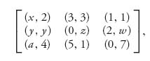
where x, y, z, w, and a are arbitrary.
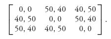
3.18 Two radio stations (WSUP and WHAP) have to choose formats for their broadcasts. There are three possible formats: Rhythm and Blues (RB), Elevator Music (EM), or all talk (AT). The audiences for the three formats are 50%, 30%, and 20%, respectively. If they choose the same formats they will split the audience for that format equally, while if they choose different formats, each will get the total audience for that format.
3.19 In a modified story of the prodigal son, a man had two sons, the prodigal and the one who stayed home. The man gave the prodigal son his share of the estate, which he squandered, and told the son who stayed home that all that he (the father) has is his (the son’s). When the man died, the prodigal son again wanted his share of the estate. They each tell the judge (it ends up in court) a share amount they would be willing to take, either ![]() ,
, ![]() , or
, or ![]() . Call the shares for each player Ii, IIi, i = 1, 2, 3. If Ii + IIj > 1, all the money goes to the game theory society. If Ii + IIj ≤ 1, then each gets the share they asked for and the rest goes to an antismoking group.
. Call the shares for each player Ii, IIi, i = 1, 2, 3. If Ii + IIj > 1, all the money goes to the game theory society. If Ii + IIj ≤ 1, then each gets the share they asked for and the rest goes to an antismoking group.
3.20 Willard is a salesman with an expense account for travel. He can steal (S) from the account by claiming false expenses or be honest (H) and accurately claim the expenses incurred. Willard’s boss is Fillmore. Fillmore can check (C) into the expenses claimed or trust (T) that Willard is honest. If Willard cheats on his expenses he benefits by the amount b assuming he isn’t caught by Fillmore. If Fillmore doesn’t check then Willard gets away with cheating. If Willard is caught cheating he incurs costs p which may include getting fired and paying back the amount he stole. Since Willard is a clever thief, we let 0 < α < 1 be the probability that Willard is caught if Fillmore investigates.
If Fillmore investigates he incurs cost c no matter what. Finally, let λ be Fillmore’s loss if Willard cheats on his expenses but is not caught. Assume all of b, p, α, λ > 0.
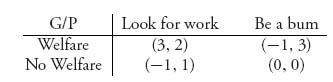
3.21 Use the equality of payoffs Theorem 3.2 to solve the welfare game. In the welfare game the state, or government, wants to aid a pauper if he is looking for work but not otherwise. The pauper looks for work only if he cannot depend on welfare, but he may not be able to find a job even if he looks. The game matrix is
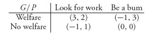
Find all Nash equilibria and graph the rational reaction sets.
3.3 Interior Mixed Nash Points by Calculus
Whenever we are faced with a problem of maximizing or minimizing a function, we are taught in calculus that we can find them by finding critical points and then trying to verify that they are minima or maxima or saddle points. Of course, a critical point doesn’t have to be any of these special points. When we look for Nash equilibria that simply supply the maximum expected payoff, assuming that the other players are doing the same for their payoffs, why not apply calculus? That’s exactly what we can do, and it will give us all the interior, that is, completely mixed Nash points. The reason it works here is because of the nature of functions like f(x, y) = X AYT. Calculus cannot give us the pure Nash equilibria because those are achieved on the boundary of the strategy region.
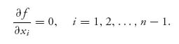
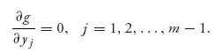
The easy part in applying calculus is to find the partial derivatives, set them equal to zero, and see what happens. Here is the procedure.
3.3.1 CALCULUS METHOD FOR INTERIOR NASH
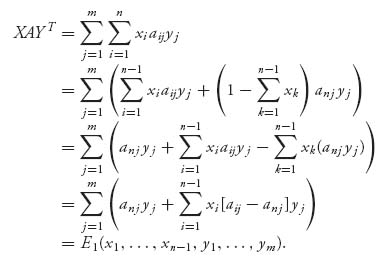
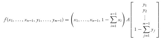
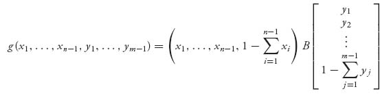
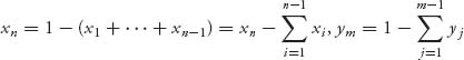 so each expected payoff is a function only of x1, …, xn−1, y1, …, ym−1. We can write
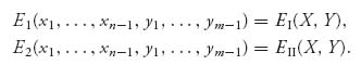
It is important to observe that we do not maximize E1(x1, …, xn−1, y1, …, ym−1) over all variables x and y, but only over the x variables. Similarly, we do not maximize E2(x1, …, xn−1, y1, …, ym−1) over all variables x and y, but only over the y variables. A Nash equilibrium for a player is a maximum of the player’s payoff over those variables that player controls, assuming that the other player’s variables are held fixed.
Example 3.9 The bimatrix game we considered in the preceding section had the two matrices
What happens if we use the calculus method on this game? First, set up the functions (using X = (X, 1 − x), Y = (y, 1 − y))
Player I wants to maximize E1 for each fixed y, so we take
Similarly, player II wants to maximize E2(x, y) for each fixed x, so
Everything works to give us ![]() and
and ![]() is a Nash equilibrium for the game, just as we had before. We do not get the pure Nash points for this problem. But those are easy to get by determining the pairs of payoffs that are simultaneously the largest in the column and the largest in the row, just as we did before. We don’t need calculus for that.
is a Nash equilibrium for the game, just as we had before. We do not get the pure Nash points for this problem. But those are easy to get by determining the pairs of payoffs that are simultaneously the largest in the column and the largest in the row, just as we did before. We don’t need calculus for that.
Example 3.10 Two partners have two choices for where to invest their money, say, O1, O2 where the letter O stands for opportunity, but they have to come to an agreement. If they do not agree on joint investment, there is no benefit to either player. We model this using the bimatrix
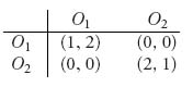
If player I chooses O1 and II chooses O1 the payoff to I is 1 and the payoff to II is 2 units because II prefers to invest the money into O1 more than into O2. If the players do not agree on how to invest, then each receives 0.
To solve this game, first notice that there are two pure Nash points at (O1, O1) and (O2, O2), so total cooperation will be a Nash equilibrium. We want to know if there are any mixed Nash points. We will start the analysis from the beginning rather than using the formulas from Section 3.2. The reader should verify that our result will match if we do use the formulas. We will derive the rational reaction sets for each player directly.
Set
Then player I’s expected payoff (using X = (x, 1 − x), Y = (y, 1 − y)) is
Keep in mind that player I wants to make this as large as possible for any fixed 0 ≤ y ≤ 1. We need to find the maximum of E1 as a function of x ![]() [0, 1] for each fixed y
[0, 1] for each fixed y ![]() [0, 1].
[0, 1].
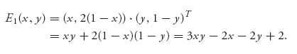
Write E1 as
![]()
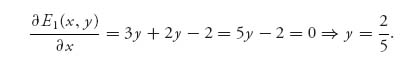
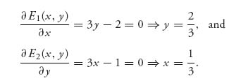
If 3y − 2 > 0, then E1(x, y) is maximized as a function of x at x = 1. If 3y − 2 < 0, then the maximum of E1(x, y) will occur at x = 0. If 3y − 2 = 0, then y = ![]() and E1(x,
and E1(x, ![]() ) =
) = ![]() ; that is, we have shown that
; that is, we have shown that
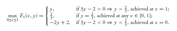
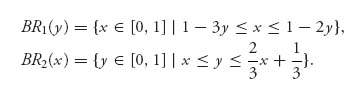
Recall that the set of points where the maximum is achieved by player I for each fixed y for player II is the rational reaction set for player I:
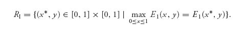
In this example, we have shown that
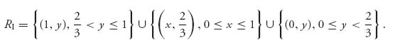
This is the rational reaction set for player I because no matter what II plays, player I should use an (x, y) ![]() RI. For example, if y =
RI. For example, if y = ![]() , then player I should use x = 0 and I receives payoff E(0,
, then player I should use x = 0 and I receives payoff E(0, ![]() ) = 1; if y =
) = 1; if y = ![]() , then I should choose x = 1 and I receives E1(1,
, then I should choose x = 1 and I receives E1(1, ![]() ) =
) = ![]() ; and when y =
; and when y = ![]() , it doesn’t matter what player I chooses because the payoff to I will be exactly
, it doesn’t matter what player I chooses because the payoff to I will be exactly ![]() for any x
for any x ![]() [0, 1].
[0, 1].
Next, we consider E2(x, y) in a similar way. Write
![]()
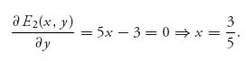
Player II wants to choose y ![]() [0, 1] to maximize this, and that will depend on the coefficient of y, namely, 3x − 1. We see as before that
[0, 1] to maximize this, and that will depend on the coefficient of y, namely, 3x − 1. We see as before that
The rational reaction set for player II is the set of points where the maximum is achieved by player II for each fixed x for player II:
We see that in this example
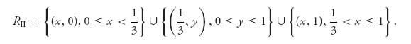
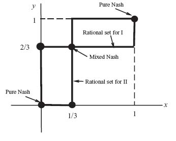
Figure 3.3 is the graph of RI and RII on the same set of axes:
The zigzag lines form the rational reaction sets of the players. For example, if player I decides for some reason to play O1 with probability x = ![]() , then player II would rationally play y = 1. Where the zigzag lines cross (which is the set of points RI
, then player II would rationally play y = 1. Where the zigzag lines cross (which is the set of points RI ![]() RII) are all the Nash points; that is, the Nash points are at (x, y) = (0, 0), (1, 1), and (
RII) are all the Nash points; that is, the Nash points are at (x, y) = (0, 0), (1, 1), and (![]() ,
, ![]() ). So either they should always cooperate to the advantage of one player or the other, or player I should play O1 one-third of the time and player II should play O1 two-thirds of the time. The associated expected payoffs are as follows:
). So either they should always cooperate to the advantage of one player or the other, or player I should play O1 one-third of the time and player II should play O1 two-thirds of the time. The associated expected payoffs are as follows:
and
Only the mixed strategy Nash point (X*, Y*) = ((![]() ,
, ![]() ), (
), (![]() ,
, ![]() )) gives the same expected payoffs to the two players. This seems to be a problem. Only the mixed strategy gives the same payoff to each player, but it will result in less for each player than they could get if they play the pure Nash points. Permitting the other player the advantage results in a bigger payoff to both players! If one player decides to cave, they both can do better, but if both players insist that the outcome be fair, whatever that means, then they both do worse.
)) gives the same expected payoffs to the two players. This seems to be a problem. Only the mixed strategy gives the same payoff to each player, but it will result in less for each player than they could get if they play the pure Nash points. Permitting the other player the advantage results in a bigger payoff to both players! If one player decides to cave, they both can do better, but if both players insist that the outcome be fair, whatever that means, then they both do worse.
Calculus will give us the interior mixed Nash very easily:
The method of solution we used in this example gives us the entire rational reaction set for each player. It is essentially the way Proposition 3.2.3 was proved.
Another point to notice is that the rational reaction sets and their graphs do not indicate what the payoffs are to the individual players, only what their strategies should be.
FIGURE 3.3 Rational reaction sets for both players.
Finally, we record here the definition of the rational reaction sets in the general case with arbitrary size matrices.
Definition 3.3.1 The rational reaction sets for each player are defined as follows:
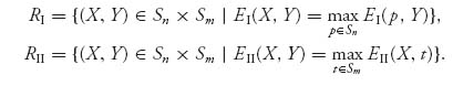
The set of all Nash equilibria is then the set of all common points RI ![]() RII.
RII.
We can write down the system of equations that we get using calculus in the general case, after taking the partial derivatives and setting to zero. We start with
Following the calculus method, we replace3 ![]() and do some algebra:
and do some algebra:
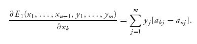
But then, for each k = 1, 2, …, n − 1, we obtain
Similarly, for each s = 1, 2, …, m − 1, we get the partials
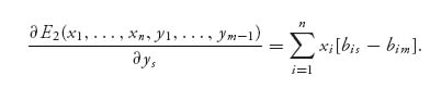
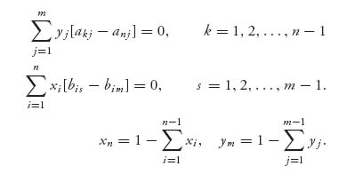
So, the system of equations we need to solve to get an interior Nash equilibrium is
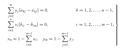
Once these are solved, we check that xi ≥ 0, yj ≥ 0. If these all check out, we have found a Nash equilibrium X* = (x1, …, xn) and Y* = (y1, …, ym). Note also that the equations are really two separate systems of linear equations and can be solved separately because the variables xi and yj appear only in their own system. Also note that these equations are really nothing more than the equality of payoffs Theorem 3.2.4, because, for example,
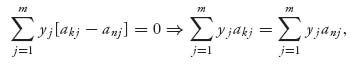
which is the same as saying that for k = 1, 2, …, n − 1, we have
All the payoffs are equal. This, of course, assumes that each row of A is used by player I with positive probability in a Nash equilibrium, but that is our assumption about an interior Nash equilibrium. These equations won’t necessarily work for the pure Nash or the ones with zero components.
It is not recommended that you memorize these equations but rather that you start from scratch on each problem.
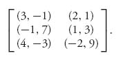
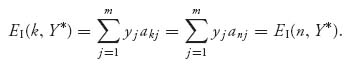
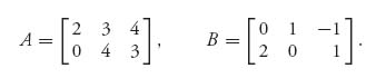
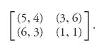
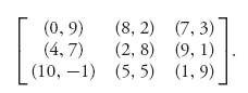
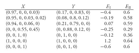
Example 3.11 We are going to use the equations (3.1) to find interior Nash points for the following bimatrix game:
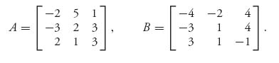
The system of equations (3.1) for an interior Nash point become
![]()
and
![]()
There is one and only one solution given by y1 = ![]() , y2 =
, y2 = ![]() and x1 =
and x1 = ![]() , x2 =
, x2 = ![]() , so we have y3 =
, so we have y3 = ![]() , x3 =
, x3 = ![]() , and our interior Nash point is
, and our interior Nash point is
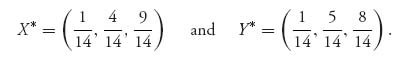
The expected payoffs to each player are EI(X*, Y*) = X* AY*T = ![]() and EII(X*, Y*) = X* BY*T =
and EII(X*, Y*) = X* BY*T = ![]() . It appears that player I does a lot better in this game with this Nash.
. It appears that player I does a lot better in this game with this Nash.
We have found the interior, or mixed Nash point. There are also two pure Nash points and they are X* = (0, 0, 1), Y* = (1, 0, 0) with payoffs (2, 3) and X* = (0, 1, 0), Y* = (0, 0, 1) with payoffs (3, 4). With multiple Nash points, the game can take on one of many forms.
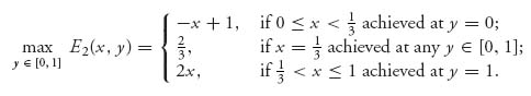
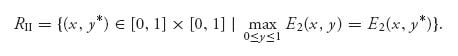
Example 3.12 Here is a last example in which the equations do not work (see Problem 3.22) because it turns out that one of the columns should never be played by player II. That means that the mixed Nash is not in the interior, but on the boundary of Sn × Sm.
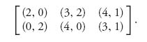
Let’s consider the game with payoff matrices
You can calculate that the safety levels are value(A) = 2, with pure saddle XA = (1, 0), YA = (1, 0, 0), and value(BT) = ![]() , with saddle XB = (
, with saddle XB = (![]() ,
, ![]() , 0), YB = (
, 0), YB = (![]() ,
, ![]() ). These are the amounts that each player can get assuming that both are playing in a zero sum game with the two matrices.
). These are the amounts that each player can get assuming that both are playing in a zero sum game with the two matrices.
Now, let X = (x, 1 − x), Y = (y1, y2, 1 − y1 − y2) be a Nash point for the bimatrix game. Calculate
![]()
Player I wants to maximize E1(x, y1, y2) for given fixed y1, y2 ![]() [0, 1], y1 + y2 ≤ 1, using x
[0, 1], y1 + y2 ≤ 1, using x ![]() [0, 1]. So we look for maxx E1(x, y1, y2). For fixed y1, y2, we see that E1(x, y1, y2) is a straight line with slope y1 − 2y2 + 1. The maximum of that line will occur at an endpoint depending on the sign of the slope. Here is what we get:
[0, 1]. So we look for maxx E1(x, y1, y2). For fixed y1, y2, we see that E1(x, y1, y2) is a straight line with slope y1 − 2y2 + 1. The maximum of that line will occur at an endpoint depending on the sign of the slope. Here is what we get:
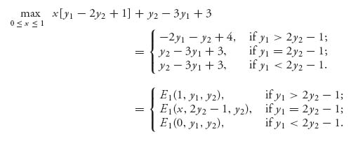
Along any point of the straight line y1 = 2y2 − 1 the maximum of E1(x, y1, y2) is achieved at any point 0 ≤ x ≤ 1. We end up with the following set of maximums for E1(x, y1, y2):
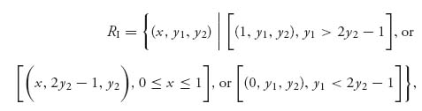
which is exactly the rational reaction set for player I. This is a set in three dimensions.
Now we go through the same procedure for player II, for whom we calculate,
![]()
Player II wants to maximize E2(x, y1, y2) for given fixed x ![]() [0, 1] using y1, y2
[0, 1] using y1, y2 ![]() [0, 1], y1 + y2 ≤ 1. We look for maxy1, y2 E2(x, y1, y2).
[0, 1], y1 + y2 ≤ 1. We look for maxy1, y2 E2(x, y1, y2).
Here is what we get:
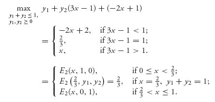
To explain where this came from, let’s consider the case 3x − 1 < 1. In this case, the coefficient of y2 is less than the coefficient of y1 (which is 1), so the maximum will be achieved by taking y2 = 0 and y1 = 1 because that gives the biggest weight to the largest coefficient. Then plugging in y1 = 1, y2 = 0 gives payoff −2x + 2. If 3x − 1 = 1, the coefficients of y1 and y2 are the same, then we can take any y1 and y2 as long as y1 + y2 = 1. Then the payoff becomes (y1 + y2)(3x − 1) + (−2x + 1) = x, but 3x − 1 = 1 requires that x = ![]() , so the payoff is
, so the payoff is ![]() . The case 3x − 1 > 1 is similar.
. The case 3x − 1 > 1 is similar.
We end up with the following set of maximums for E2(x, y1, y2):
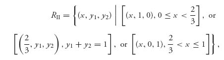
which is the rational reaction set for player II.
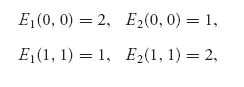
The graph of RI and RII on the same graph (in three dimensions) will intersect at the mixed Nash equilibrium points. In this example, the Nash equilibrium is given by
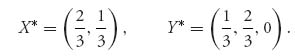
Then, E1(![]() ,
, ![]() ,
, ![]() ) =
) = ![]() and E2(
and E2(![]() ,
, ![]() ,
, ![]() ) =
) = ![]() are the payoffs to each player. We could have simplified the calculations significantly if we had noticed from the beginning that we could have eliminated the third column from the bimatrix because column 3 for player II is dominated by column 1, and so may be dropped.
are the payoffs to each player. We could have simplified the calculations significantly if we had noticed from the beginning that we could have eliminated the third column from the bimatrix because column 3 for player II is dominated by column 1, and so may be dropped.
Problems
3.22 Write down the equations (3.1) for the game
Try to solve the equations. What, if anything, goes wrong?
3.23 The game matrix in the welfare problem is
Write the system of equations for an interior Nash and solve them.
3.24 Consider the game with bimatrix
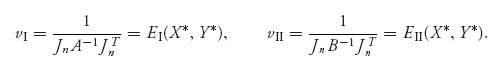
3.25 In this problem, we consider the analogue of the invertible matrix Theorem 2.2.1 for zero sum games. Consider the nonzero sum game (An×n, Bn×n) and suppose that A−1 and B−1 exist.
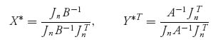
are strategies, then (X*, Y*) is a Nash equilibrium, and
3.26 Chicken game. In this version of the game, the matrix is
Find the mixed Nash equilibrium and show that as a > 0 increases, so does the expected payoff to each player under the mixed Nash.
3.27 Find all possible Nash equilibria for the game and the rational reaction sets:
Consider all cases (a > 0, b > 0), (a > 0, b < 0), and so on.
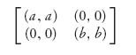
3.28 Show that a 2 × 2 symmetric game
has exactly the same set of Nash equilibria as does the symmetric game with matrix
for any a, b.
3.29 Consider the game with matrix
3.30 A game called the battle of the sexes is a game between a husband and wife trying to decide about cooperation. On a given evening, the husband wants to see wrestling at the stadium, while the wife wants to attend a concert at orchestra hall. Neither the husband nor the wife wants to go to what the other has chosen, but neither do they want to go alone to their preferred choice. They view this as a two-person nonzero sum game with matrix
If they decide to cooperate and both go to wrestling, the husband receives 2 and the wife receives 1, because the husband gets what he wants and the wife partially gets what she wants. The rest are explained similarly. This is a model of compromise and cooperation. Use the method of this section to find all Nash equilibria. Graph the rational reaction sets.
3.31 Hawk–Dove Game. Two companies both want to take over a sales territory. They have the choices of defending the territory and fighting if necessary, or act as if willing to fight but if the opponent fights (F), then backing off (Bo). They look at this as a two-person nonzero sum game with matrix
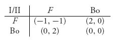
Solve this game and graph the rational reaction sets.
3.32 Stag–Hare Game. Two hunters are pursuing a stag. Each hunter has the choice of going after the stag (S), which will be caught if they both go after it and it will be shared equally, or peeling off and going after a rabbit (R). Only one hunter is needed to catch the rabbit and it will not be shared. Look at this as a nonzero sum two-person game with matrix
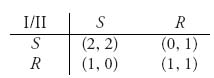
This assumes that they each prefer stag meat to rabbit meat, and they will each catch a rabbit if they decide to peel off. Solve this game and graph the rational reaction sets.
3.33 We are given the following game matrix.
3.3.2 PROOF THAT THERE IS A NASH EQUILIBRIUM FOR BIMATRIX GAMES (OPTIONAL)
The set of all Nash equilibria is determined by the set of all common points RI ![]() RII. How do we know whether this intersection has any points at all? It might have occurred to you that we have no guarantee that looking for a Nash equilibrium in a bimatrix game with matrices (A, B) would ever be successful. So maybe we need a guarantee that what we are looking for actually exists. That is what Nash’s theorem gives us.
RII. How do we know whether this intersection has any points at all? It might have occurred to you that we have no guarantee that looking for a Nash equilibrium in a bimatrix game with matrices (A, B) would ever be successful. So maybe we need a guarantee that what we are looking for actually exists. That is what Nash’s theorem gives us.
Theorem 3.3.2 There exists X* ![]() Sn and Y*
Sn and Y* ![]() Sm so that
Sm so that
for any other mixed strategies X ![]() Sn, Y
Sn, Y ![]() Sm.
Sm.
The theorem guarantees at least one Nash equilibrium if we are willing to use mixed strategies. In the zero sum case, this theorem reduces to von Neumann’s minimax theorem.
Proof. We will give a proof that is very similar to that of von Neumann’s theorem using the Kakutani fixed-point theorem for point to set maps, but there are many other proofs that have been developed, as is true of many theorems that are important. As we go through this, note the similarities with the proof of von Neumann’s theorem.
First Sn × Sm is a closed, bounded and convex set. Now for each given pair of strategies (X, Y), we could consider the best response of player II to X and the best response of player I to Y. In general, there may be more than one best response, so we consider the best response sets. Here's the definition of a best response set.
Definition 3.3.3 The best response sets for each player are defined as
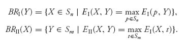
The difference between the best response set and the rational reaction set is that the rational reaction set RI consists of the pairs of strategies (X, Y) for which EI(X, Y) = maxp EI(p, Y), whereas the set BRI(Y) consists of the strategy (or collection of strategies) X for player I that is the best response to a fixed Y. Whenever you are maximizing a continuous function, which is true of EI(X, Y), over a closed and bounded set (which is true of Sn), you always have a point at which the maximum is achieved. So we know that BRI(Y) ≠ ![]() . Similarly, the same is true of BRII(X) ≠
. Similarly, the same is true of BRII(X) ≠ ![]() .
.
We define the point to set mapping
![]()
which gives, for each pair (X, Y) of mixed strategies, a pair of best response strategies (X′, Y′) ![]()
![]() (X, Y) with X′
(X, Y) with X′ ![]() BRI(Y) and Y′
BRI(Y) and Y′ ![]() BRII(X).
BRII(X).
It seems natural that our Nash equilibrium should be among the best response strategies to the opponent. Translated, this means that a Nash equilibrium (X*, Y*) should satisfy (X*, Y*) ![]()
![]() (X*, Y*). But that is exactly what it means to be a fixed point of
(X*, Y*). But that is exactly what it means to be a fixed point of ![]() . If
. If ![]() satisfies the required properties to apply Kakutani’s fixed-point theorem, we have the existence of a Nash equilibrium. This is relatively easy to check because X
satisfies the required properties to apply Kakutani’s fixed-point theorem, we have the existence of a Nash equilibrium. This is relatively easy to check because X ![]() EI(X, Y) and X
EI(X, Y) and X ![]() EII(X, Y) are linear maps, as are Y
EII(X, Y) are linear maps, as are Y ![]() EI(X, Y) and Y
EI(X, Y) and Y ![]() EII(X, Y). Hence, it is easy to show that
EII(X, Y). Hence, it is easy to show that ![]() (X, Y) is a convex, closed, and bounded subset of Sn × Sm. It is also not hard to show that
(X, Y) is a convex, closed, and bounded subset of Sn × Sm. It is also not hard to show that ![]() will be an (upper) semicontinuous map, and so Kakutani’s theorem applies.
will be an (upper) semicontinuous map, and so Kakutani’s theorem applies.
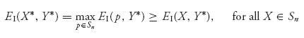
This gives us a pair (X*, Y*) ![]()
![]() (X*, Y*). Written out, this means X*
(X*, Y*). Written out, this means X* ![]() BRI(Y*) so that
BRI(Y*) so that
and Y* ![]() BRII(X*) so that
BRII(X*) so that
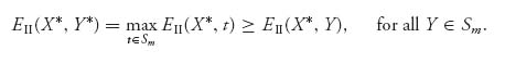
That’s it. (X*, Y*) is a Nash equilibrium. ![]()
Finally, it is important to understand the difficulty in obtaining the existence of a Nash equilibrium. If our problem was
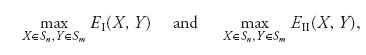
then the existence of an (XI, YI) providing the maximum of EI is immediate from the fact that EI(X, Y) is a continuous function over a closed and bounded set. The same is true for the existence of an (XII, YII) providing the maximum of EII(X, Y). The problem is that we don’t know whether XI = XII and YI = YII. In fact, that is very unlikely and it is a stronger condition than what is required of a Nash equilibrium.
3.4 Nonlinear Programming Method for Nonzero Sum Two-Person Games
We have shown how to calculate the pure Nash equilibria in the 2 × 2 case, and the system of equations that will give a mixed Nash equilibrium in more general cases. In this section, we present a method (introduced by Lemke and Howson (1964) in the 1960s) of finding all Nash equilibria for arbitrary two-person nonzero sum games with any number of strategies. We formulate the problem of finding a Nash equilibrium as a nonlinear program, in contrast to the formulation of solution of a zero sum game as a linear program.
In general, a nonlinear program is simply an optimization problem involving nonlinear functions and nonlinear constraints. For example, if we have an objective function f and constraint functions h1, …, hK, the problem
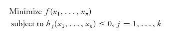
is a fairly general formulation of a nonlinear programming problem. In general, the functions f, hj are not linear, but they could be. In that case, of course, we have a linear program, which is solved by the simplex algorithm. If the function f is quadratic and the constraint functions are linear, then this is called a quadratic programming problem and special techniques are available for those. Nonlinear programs are more general and the techniques to solve them are more involved, but fortunately there are several methods available, both theoretical and numerical. Nonlinear programming is a major branch of operations research and is under very active development. In our case, once we formulate the game as a nonlinear program, we will use the packages developed in Maple/Mathematica to solve them numerically. The first step is to set it up.
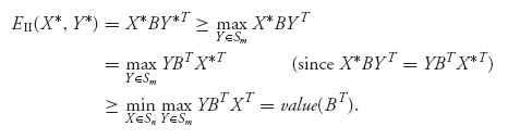
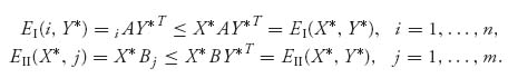
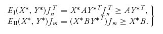
Theorem 3.4.1 Consider the two-person game with matrices (A, B) for players I and II. Then, (X* ![]() Sn, Y*
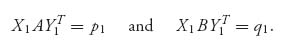
Sn, Y* ![]() Sm) is a Nash equilibrium if and only if they satisfy, along with scalars p*, q* the nonlinear program
Sm) is a Nash equilibrium if and only if they satisfy, along with scalars p*, q* the nonlinear program
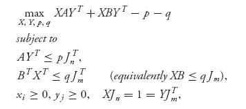
where Jk = (1 1 1 … 1) is the 1 × k row vector consisting of all 1s. In addition, p* = EI(X*, Y*) and q* = EII(X*, Y*).
Remark Expanded, this program reads as
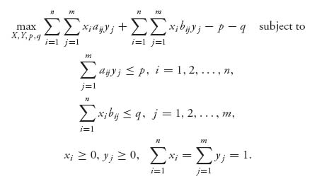
You can see that this is a nonlinear program because of the presence of the terms xiyj. That is why we need a nonlinear programming method, or a quadratic programming method because it falls into that category.
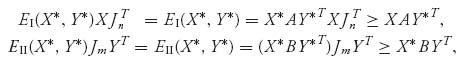
Proof. Here is how the proof of this useful result goes. Recall that a strategy pair (X*, Y*) is a Nash equilibrium if and only if
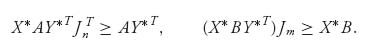
Keep in mind that the quantities EI(X*, Y*) and EII(X*, Y*) are scalars. In the first inequality of (3.2), successively choose X = (0, …, 1, …, 0) with 1 in each of the n spots, and in the second inequality of (3.2) choose Y = (0, …, 1, …, 0) with 1 in each of the m spots, and we see that EI(X*, Y*) ≥ EI(i, Y*) = iAY*T for each i, and EII(X*, Y*) ≥ EII(X*, j) = X* Bj, for each j. In matrix form, this is
However, it is also true that if (3.3) holds for a pair (X*, Y*) of strategies, then these strategies must be a Nash point, that is, (3.2) must be true. Why? Well, if (3.3) is true, we choose any X ![]() Sn and Y
Sn and Y ![]() Sm and multiply
Sm and multiply
because ![]() . But this is exactly what it means to be a Nash point. This means that (X*, Y*) is a Nash point if and only if
. But this is exactly what it means to be a Nash point. This means that (X*, Y*) is a Nash point if and only if
We have already seen this in Proposition 3.2.2.
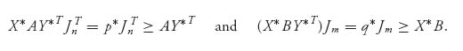
Now suppose that (X*, Y*) is a Nash point. We will see that if we choose the scalars
![]()
then (X*, Y*, p*, q*) is a solution of the nonlinear program. To see this, we first show that all the constraints are satisfied. In fact, by the equivalent characterization of a Nash point we just derived, we get
The rest of the constraints are satisfied because X* ![]() Sn and Y*
Sn and Y* ![]() Sm. In the language of nonlinear programming, we have shown that (X*, Y*, p*, q*) is a feasible point. The feasible set is the set of all points that satisfy the constraints in the nonlinear programming problem.
Sm. In the language of nonlinear programming, we have shown that (X*, Y*, p*, q*) is a feasible point. The feasible set is the set of all points that satisfy the constraints in the nonlinear programming problem.
We have left to show that (X*, Y*, p*, q*) maximizes the objective function
![]()
over the set of the possible feasible points.
Since every feasible solution (meaning it maximizes the objective over the feasible set) to the nonlinear programming problem must satisfy the constraints ![]() and XB ≤ q Jm, multiply the first on the left by X and the second on the right by YT to get
and XB ≤ q Jm, multiply the first on the left by X and the second on the right by YT to get
![]()
Hence, any possible solution gives the objective
![]()
So f(X, Y, p, q) ≤ 0 for any feasible point. But with p* = X* AY*T, q* = X* BY*T, we have seen that (X*, Y*, p*, q*) is a feasible solution of the nonlinear programming problem and

by definition of p* and q*. Hence, this point (X*, Y*, p*, q*) both is feasible and gives the maximum objective (which we know is zero) over any possible feasible solution and so is a solution of the nonlinear programming problem. This shows that if we have a Nash point, it must solve the nonlinear programming problem.
Now we have to show the reverse, namely, that any solution of the nonlinear programming problem must be a Nash point (and we get the optimal expected payoffs as well).
For the opposite direction, let X1, Y1, p1, q1 be any solution of the nonlinear programming problem, let (X*, Y*) be a Nash point for the game, and set p* = X* AY*T, q* = X* BY*T. We will show that (X1, Y1) must be a Nash equilibrium of the game.
Since X1, Y1 satisfy the constraints of the nonlinear program ![]() and X1 B ≤ q1 Jm, we get, by multiplying the constraints appropriately
and X1 B ≤ q1 Jm, we get, by multiplying the constraints appropriately
![]()
Now, we know that if we use the Nash point (X*, Y*) and p* = X* AY*T, q* = X* BY*T, then f(X*, Y*, p*, q*) = 0, so zero is the maximum objective. But we have just shown that our solution to the program (X1, Y1, p1, q1) satisfies f(X1, Y1, p1, q1) ≤ 0. Consequently, it must in fact be equal to zero:
![]()
The terms in parentheses are nonpositive, and the two terms add up to zero. That can happen only if they are each zero. Hence,
Then we write the constraints as
![]()
However, we have shown at the beginning of this proof that this condition is exactly the same as the condition that (X1, Y1) is a Nash point. So that’s it; we have shown that any solution of the nonlinear program must give a Nash point, and the scalars must be the expected payoffs using that Nash point. ![]()
Remark It is not necessarily true that EI(X1, Y1) = p1 = p* = EI(X*, Y*) and EII(X1, Y1) = q1 = q* = EII(X*, Y*). Different Nash points can, and usually do, give different expected payoffs, as we have seen many times.
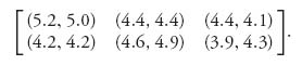
Using this theorem and some nonlinear programming implemented in Maple or Mathematica, we can numerically solve any two-person nonzero sum game. For an example, suppose that we have the matrices
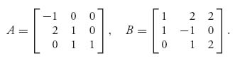
Now, before you get started looking for mixed Nash points, you should first find the pure Nash points. For this game, we have two Nash points at (X1 = (0, 1, 0), Y1 = (1, 0, 0)) with expected payoff ![]() , and (X2 = (0, 0, 1) = Y2) with expected payoffs
, and (X2 = (0, 0, 1) = Y2) with expected payoffs ![]() .
.
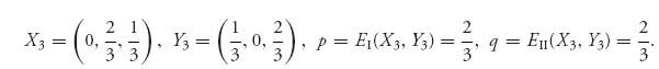
On the other hand, we may solve the nonlinear programming problem with these matrices and obtain a mixed Nash point
Here are the Maple commands to get the solutions:
> with(LinearAlgebra):
> A:=Matrix([[-1, 0, 0], [2, 1, 0], [0, 1, 1]]);
> B:=Matrix([[1, 2, 2], [1, -1, 0], [0, 1, 2]]);
> X:=<x[1], x[2], x[3]>; #Or X:=Vector(3, symbol=x):
> Y:=<y[1], y[2], y[3]>; #Or Y:=Vector(3, symbol=y):
> Cnst:={seq((A.Y)[i]<=p, i=1..3),
         seq((Transpose(X).B)[i]<=q, i=1..3),
         add(x[i], i=1..3)=1, add(y[i], i=1..3)=1};
> with(Optimization);
> objective:=expand(Transpose(X).A.Y+Transpose(X).B.Y-p-q);
> QPSolve(objective, Cnst, assume=nonnegative, maximize);
> QPSolve(objective, Cnst, assume=nonnegative, maximize,
                               initialpoint=({q=1, p=2}));
> NLPSolve(objective, Cnst, assume=nonnegative, maximize);
This gives us the result p = 0.66, q = 0.66, x[1] = 0, x[2] = 0.66, x[3] = 0.33 and y[1] = 0.33, y[2] = 0, y[3] = 0.66. The commands also tell us that the value of the objective function at the optimal points is zero, which is what the theorem guarantees, namely, max f(X, Y, p, q) = 0. By changing the initial point, which is indicated with the option initialpoint=({q=1, p=2}), we may also find the pure Nash solution X = (0, 1, 0) and Y = (1, 0, 0). This is rather a waste, however, because there is no need to use a computer to find the pure Nash points unless it is a very large game. Nevertheless, if you see a solution that seems to be pure, you could check it directly.
The commands indicate there are two ways Maple can solve this problem. First, recognizing the payoff objective function as a quadratic function, we can use the command QPSolve which specializes to quadratic programming problems and is faster. Second, in general for any nonlinear objective function we use NLPSolve.
You do have to make one change to the Maple commands if the expected payoffs of the game can be negative. The commands
>QPSolve(objective, Cnst, assume=nonnegative, maximize,
                               initialpoint=({q=1, p=2}));
>NLPSolve(objective, Cnst, assume=nonnegative, maximize);
are set up assuming that all variables including p and q are nonnegative. If they can possibly be negative, then these commands will not find the Nash equilibria associated with negative payoffs. It is not a big deal, but we have to drop the assume=nonnegative part of these commands and add the nonnegativity of the strategy variables to the constraints. Here is what you need to do:
> with(LinearAlgebra):
> A:=Matrix([[-1, 0, 0], [2, 1, 0], [0, 1, 1]]);
> B:=Matrix([[1, 2, 2], [1, -1, 0], [0, 1, 2]]);
> X:=<x[1], x[2], x[3]>;
> Y:=<y[1], y[2], y[3]>;
> Cnst:={seq((A.Transpose(Y))[i]<=p, i=1..3), seq((X.B)[i]<=q, i=1..3),
         add(x[i], i=1..3)=1, add(y[i], i=1..3)=1,
         seq(y[i]> = 0, i=1..3), seq(x[i]> = 0, i=1..3)};
> with(Optimization);
> objective:=expand(Transpose(X).A.Y+Transpose(X).B.Y-p-q);
> QPSolve(objective, Cnst, maximize);
> QPSolve(objective, Cnst, maximize, initialpoint=({q=1, p=2}));
> NLPSolve(objective, Cnst, maximize);
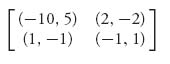
Example 3.13 Suppose that two countries are involved in an arms control negotiation. Each country can decide to either cooperate or not cooperate (don’t). For this game, one possible bimatrix payoff situation may be
This game has a pure Nash equilibrium at (2, 2), so these countries will not actually negotiate in good faith. This would lead to what we might call deadlock because the two players will decide not to cooperate. If a third party managed to intervene to change the payoffs, you might get the following payoff matrix:
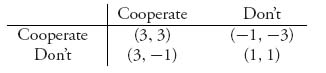
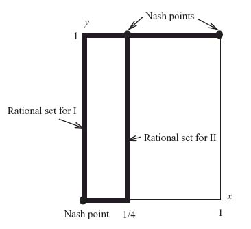
What’s happened is that both countries will receive a greater reward if they cooperate and the benefits of not cooperating on the part of both of them have decreased. In addition, we have lost symmetry. If the row player chooses to cooperate but the column player doesn’t, they both lose, but player I will lose less than player II. On the other hand, if player I doesn’t cooperate but player II does cooperate, then player I will gain and player II will lose, although not as much. Will that guarantee that they both cooperate? Not necessarily. We now have pure Nash equilibria at both (3, 3) and (1, 1). Is there also a mixed Nash equilibrium? If we apply the Maple commands, or use the calculus method, or the formulas, we obtain
Actually, by graphing the rational reaction sets we see that any mixed strategy X = (x, 1 − x), Y = (1, 0), ![]() ≤ x ≤ 1, is a Nash point (see Figure 3.4).
≤ x ≤ 1, is a Nash point (see Figure 3.4).
Each player receives the most if both cooperate, but how does one move them from Don’t Cooperate to Cooperate?
FIGURE 3.4 Rational reaction sets for both players.
Here is one last example applied to dueling.
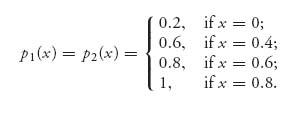
Example 3.1.4 A Discrete Silent Duel. Consider a gun duel between two persons, Pierre (player I) and Bill (player II). They each have a gun with exactly one bullet. They face each other initially 10 paces apart. They will walk toward each other, one pace at a time. At each step, including the initial one, that is, at 10 paces, they each may choose to either fire or hold. If they fire, the probability of a hit depends on how far apart they are according to the following distribution:
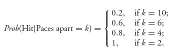
Assume in this special case that they choose to fire only at k = 10, 6, 4, 2 paces apart. It is possible for both to fire and miss, or both fire and kill.
The hardest part of the analysis is coming up with the matrices without making a computational mistake. Maple can be a big help with that. First, we define the accuracy functions
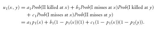
Think of 0 ≤ x ≤ 1 as the time to shoot. It is related to k by x = 1 − k/10. Now define the payoff to player I, Pierre, as
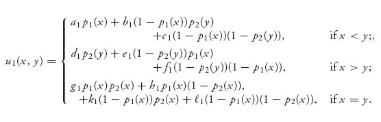
For example, if x < y, then Pierre is choosing to fire before Bill and the expected payoff is calculated as
Note that the silent part appears in the case that I misses at x and I is killed at y because the probability I is killed by II is not necessarily 1 if I misses. The remaining cases are similar.
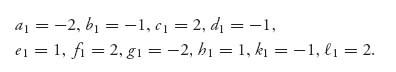
The constants multiplying the accuracy functions are the payoffs. For example, if x < y, Pierre’s payoffs are a1 if I kills II at x, b1 if I misses at x and II kills I at y, and c1 if they both miss. We have derived the payoff for player I using general payoff constants so that you may simply change the constants to see what happens with different rewards (or penalties).
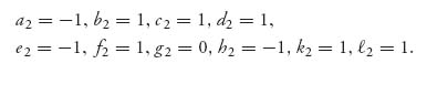
For Pierre, we will use the payoff values
The expected payoff to Bill is similarly
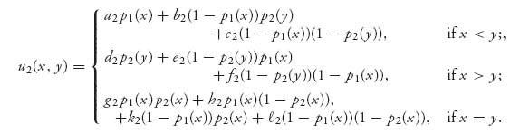
For Bill we will take the payoff values
The payoff matrix then for player I is
![]()
or
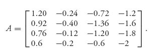
Similarly, player II’s matrix is
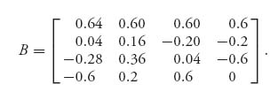
To solve this game, you may use Maple and adjust the initial point to obtain multiple equilibria. Here is the result:
It looks like the best Nash for each player is to shoot at 10 paces.
3.4.1 SUMMARY OF METHODS FOR FINDING MIXED NASH EQUILIBRIA
The methods we have for finding the mixed strategies for nonzero sum games are recapped here:
and then
This will let you find Y*. Next, compute
and then
From these you will find X*.
Problems
3.34 Consider the following bimatrix for a version of the game of chicken (see Problem 3.4):
3.35 Suppose you are told that the following is the nonlinear program for solving a game with matrices (A, B):
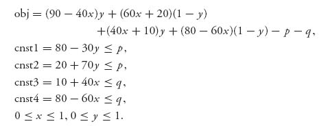
Find the associated matrices A and B and then solve the problem to find the Nash equilibrium.
3.36 Suppose that the wife in a battle of the sexes game has an additional strategy she can use to try to get the husband to go along with her to the concert, instead of wrestling. Call it strategy Z. The payoff matrix then becomes
Find all Nash equilibria.
3.37 Since every two-person zero sum game can be formulated as a bimatrix game, show how to modify the Lemke–Howson algorithm to be able to calculate saddle points of zero sum two-person games. Then use that to find the value and saddle point for the game with matrix
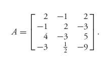
Check your answer by using the linear programming method to solve this game.
3.38 Use nonlinear programming to find all Nash equilibria for the game and expected payoffs for the game with bimatrix
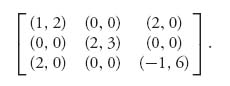
3.39 Consider the game with bimatrix
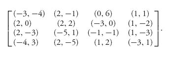
Find as many Nash equilibria as you can by adjusting the starting point in the Maple or Mathematica commands for Lemke–Howson.
3.40 Consider the gun duel between Pierre and Bill. Modify the payoff functions so that it becomes a noisy duel with a1 = −2, b1 = −1, c1 = 2, d1 = −1, e1 = 1, f1 = 2, g1 = −2, h1 = 1, k1 = −1, ![]() 1 = 2, for player I, and a2 = −1, b2 = 1, c2 = 1, d2 = 1, e2 = −1, f2 = 1, g2 = 0, h2 = −1, k2 = 1,
1 = 2, for player I, and a2 = −1, b2 = 1, c2 = 1, d2 = 1, e2 = −1, f2 = 1, g2 = 0, h2 = −1, k2 = 1, ![]() 2 = 1, for player II. Then solve the game and obtain at least one mixed Nash equilibrium.
2 = 1, for player II. Then solve the game and obtain at least one mixed Nash equilibrium.
3.5 Correlated Equilibria
A Nash equilibrium assumes that the players choose their strategies independently of one another. Frequently this is not the case. For example, in a Battle of the Sexes game it is conceivable that a husband and wife will make their decisions based on the outcome of some external event like the toss of a coin or the weather. In many situations, players choose their strategies on the basis of some random external event. Their choices of strategies would then be correlated, or, in classical probability terms, their choices are dependent. Then how do the players choose their strategies? That is what we will study in this section.
Given the game with matrices (A, B), let,
![]()
Let P be the matrix with components pij, i = 1, 2, …, n, j = 1, 2, …, m. Denote the n rows of P as iP and the m columns of P as Pj. The matrix P is called a distribution on the pure strategies of both players. In previous sections, if we have mixed strategies X = (x1, …, xn) for player I and Y = (y1, …, ym) for player II, then if the players choose independently the joint distribution is pij = xi yj.
Denote by Ij and IIk the situation in which I plays row i and II plays column j, respectively. Then pij = Prob(Ii, IIj). In the prior sections, as just mentioned, we assumed independence of the choices which would give us pij = Prob(Ii) × Prob(IIj). This assumption is now dropped.
Suppose player I plays row i. Then by the definition of conditional probability and the law of total probability, the probability player II plays IIj, given player I plays Ii is
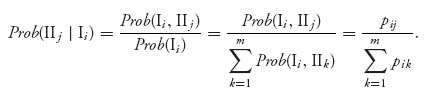
Now we calculate the expected payoff to player I, given that she plays row Ii:
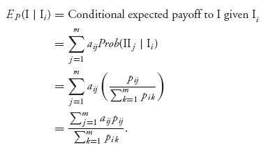
The idea now is that player I will play row i if it is a best response. In order for the distribution P = (pij) to be good for player I, the expected conditional payoff of player I given that I plays Ii should be at least as good if the payoffs for player I are switched to another row q. That is, the payoff to I, given she plays row i should be at least as good as her payoff for playing some other row q using the same information about her playing row i. In symbols,
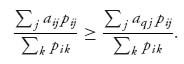
This holds because the information, given I uses Ii, does not change, but the payoffs do. Now we may cancel the denominators to get the requirement,
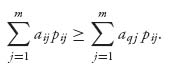
This should be true for all rows i = 1, 2, …, n, q = 1, 2, …, n.
Similarly, for player II start from the requirement that for all columns j = 1, 2, …, m
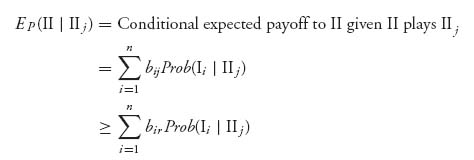
for any columns r = 1, 2, …, m, j = 1, 2, …, m. Simplifying the conditional probabilities and canceling the denominator gives
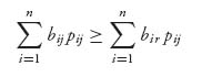
for all columns j = 1, 2, …, m, r = 1, 2, …, m.
In the 2 × 2 case we have for the correlated equilibrium matrix P
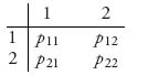
where pij is the probability player I plays row i and player II plays column j. The probability player I plays row i is pi1 + pi2. Player II will play column 1 given that player I plays row 1 with probability ![]() . If player I plays row 1 under a correlated equilibrium, her expected payoff is
. If player I plays row 1 under a correlated equilibrium, her expected payoff is
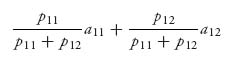
while if she deviates from playing row 1 and instead plays row 2, her payoff will be
Under a correlated equilibrium we must have
Multiplying through by p11 + p12 we have the requirement
![]()
A similar inequality must hold for the matrix B for player II. That's the way it works.
Now we can state the precise definition which is due to Robert Aumann.4
Definition 3.5.1 A distribution P = (pij) is a correlated equilibrium if
for all rows i = 1, 2, …, n, q = 1, 2, …, n, and
for all columns j = 1, 2, …, m, r = 1, 2, …, m.
Before we see how to calculate a correlated equilibrium we look at some examples.
Example 3.15 The classic example is the Game of Chicken. Consider the specific game
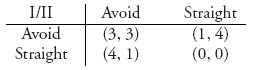
First, consider the Nash equilibria. There are two pure Nash equilibria at (4, 1) and (1, 4). There is also a single mixed Nash equilibrium X* = Y* = (![]() ,
, ![]() ) that gives payoffs (2, 2) to each player.
) that gives payoffs (2, 2) to each player.
I claim that
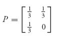
is a correlated equilibrium distribution. This means that all combinations of Avoid and Straight will be played with equal probabilities and (Straight, Straight) will never be played. By definition, we have to check if
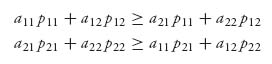
and
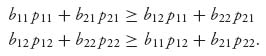
These are the general conditions for any 2 × 2 game. A compact way of remembering this is
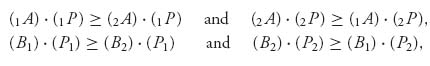
where we recall that iA is the ith row of A and Bj is the jth column of B. For our chicken, problem, we have
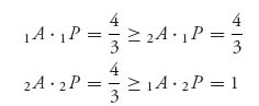
and
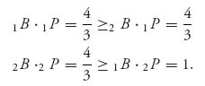
We conclude that P is indeed a correlated equilibrium. Unfortunately, it is not the only correlated equilibrium. For example, both
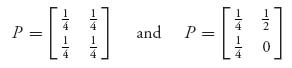
are also correlated equilibria, as you can readily check. The question is how do we find a correlated equilibrium and how do we pick out a good one.
We will set our goal as trying to make the social welfare as large as possible. Here’s what that means.
Definition 3.5.2 The social welfare payoff of a game is the maximum sum of each individual payoff. That is,
![]()
The social welfare of a pure strategy (i*, j*) is ai* j* + bi* j*.
The expected social welfare of a mixed pair (X, Y) is
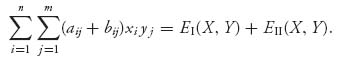
The expected social welfare of a distribution P is
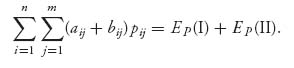
Example 3.16 (Chicken game–continued)
Each pure Nash equilibrium of the chicken game has social welfare of 5, while the mixed one gets an expected social welfare of 4, as you can easily check.
The maximum social welfare is 6 and it occurs at (Avoid, Avoid) which is not a Nash equilibrium.
If we use the correlated equilibrium ![]() , we get
, we get
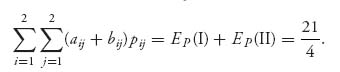
Note that the expected sum of payoffs in this correlated equilibrium is bigger than that of any Nash equilibrium. This is not necessarily the case. A correlated equilibria may give a higher or lower social welfare than any given Nash equilibrium. The question we answer is how do we find the correlated equilibrium that gives the greatest social welfare?
Remark Existence of Correlated Equilibrium. How do we know a game has a correlated equilibrium? That’s actually easy because we know that a game always has a Nash equilibrium, say (X*, Y*). To turn this into a correlated equilibrium do the following. If X* = (x1, …, xn), Y* = (y1, …, ym), set pij = xiyj and then P is the n × m matrix with elements pij. In matrix notation P = (X*)T Y*.
You now need to verify in the problems that P satisfies the definition of a correlated equilibrium. That is directly from the definitions and you will verify that in the problems.
Before we consider the problem of determining the correlated equilibrium giving the greatest social welfare let’s consider another example.
Example 3.17 Battle of the Sexes. The game between a husband and wife is given by
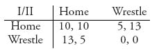
One of the spouses must stay home since they are new parents and neither trusts a baby sitter. Both would prefer to go to Wrestling if the other stays home. Each spouse must choose whether to stay Home or go Wrestling without communicating with the other spouse, that is, completely independently.
First, consider the following Nash equilibria:
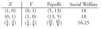
There are two equilibria in pure strategies, and a mixed equilibrium where each player goes Wrestling with probability ![]() . The expected payoff of the mixed Nash is
. The expected payoff of the mixed Nash is ![]() for each spouse. Each pure Nash gives a higher social welfare than the mixed Nash.
for each spouse. Each pure Nash gives a higher social welfare than the mixed Nash.
Suppose the two spouses agree to flip a single fair coin to decide for them. In other words, they will agree to play the distribution
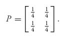
If they do that, then
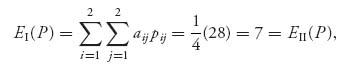
and the social welfare under P is 14.
If they were to use a biased coin that would correspond to each player using their mixed strategy, we get P = (xiyj) giving the correlated equilibrium
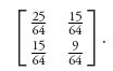
Under this distribution the social welfare is 16.25, as we expect.
Can they do better? Of course each pure Nash, if they agreed to play those, would do better. It looks like what we want is to maximize the social welfare over all possible correlated equilibria. That problem is
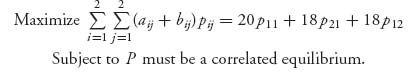
The constraints in this problem are as follows:
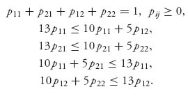
This is a linear programming problem for the unknowns P. The solution of this program gives that the maximum social welfare is achieved with the following distribution:
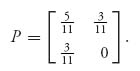
This is a correlated equilibrium giving a payoff of 9.45 to each spouse, which is better than any of the Nash equilibria and can be calculated and achieved without a prior agreement between the two players.
How do we find a correlated equilibrium in general? It turns out that finding a correlated equilibrium is actually computationally (on a computer) easier than finding a Nash equilibrium. The algorithm for a correlated equilibrium that maximizes the social welfare is very simple. It is the following linear programming problem:
3.5.1 LP PROBLEM FOR A CORRELATED EQUILIBRIUM
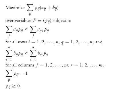
Our objective function here is chosen to be the expected social welfare of the two players, namely, EI(P) + EII(P). However, this is not the only possible objective. In fact, we may take any linear function f(P) that depends on the payoffs for each player to find a correlated equilibrium. All that is necessary for P to be a correlated equilibrium is that the constraints are satisfied. This means that in general there are many correlated equilibria of a game but we choose the one which gives both players the maximum possible payoffs.
Finally, this algorithm is easily implemented in Maple or Mathematica. Here are the Maple commands:
>restart:
>A:=Matrix([[3, 1], [4, 0]]); B:=Matrix([[3, 4], [1, 0]]);
>P:=Matrix(2, 2, symbol=p);
>P:=add(add((A[i, j]+B[i, j])*p[i, j], i=1..2), j=1..2);
>with(simplex):
>cnsts:={add(add(p[i, j], i=1..2), j=1..2)=1};
>for i from 1 to 2 do
     for k from 1 to 2 do
cnsts:=cnsts union {add(p[i, j]*A[i, j], j=1..2) >= add(p[i, j]*A[k, j], j=1..2)};
     end do;
end do;
>for j from 1 to 2 do
     for k from 1 to 2 do
cnsts:=cnsts union {add(p[i, j]*B[i, j], i=1..2) >= add(p[i, j]*B[i, k], i=1..2)};
     end do;
end do;
>maximize(P, cnsts, NONNEGATIVE); #This gives the solution.

>#Another way which uses floating point
>with(Optimization):
>LPSolve(P, cnsts, assume=nonnegative, maximize);
Here are the commands using Mathematica for our Battle of the Sexes problem:
A={{10, 5}, {13, 0}}
B={{10, 13}, {5, 0}}
P = {{p11, p12}, {p21, p22}}
Maximize[
  {Sum[Sum[(A[[i, j]] + B[[i, j]]) P[[i, j]], {j, 1, 2}], {i, 1, 2}],
 A[[1]].P[[1]] >= A[[2]].P[[1]],
 A[[2]].P[[2]] >= A[[1]].P[[2]],
 B[[All, 1]].P[[All, 1]] >= B[[All, 2]].P[[All, 1]],
 B[[All, 2]].P[[All, 2]] >= B[[All, 1]].P[[All, 2]],
 p11 + p12 + p21 + p22 == 1,
 p11 >= 0, p22 >= 0, p12 >= 0, p21 >= 0},
 {q11, q12, q21, q22}]
Mathematica gives us that the maximum is ![]() achieved at
achieved at
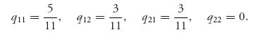
Problems
3.41 Let A, B be 2 × 2 games and P2 × 2 = (pij) a probability distribution. Show that P is a correlated equilibrium if and only if
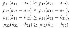
The payoffs in terms of expected social welfare are as follows:
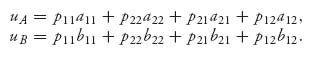
3.42 Verify that if (X*, Y*) is a Nash equilibrium for the game (A, B), then P = (X*)T Y* = (xiyj) is a correlated equilibrium.
3.43 Consider the following game of chicken:
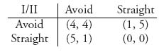
Show that the following are all correlated equilibria of this game:
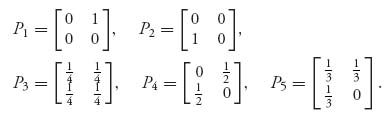
Show also that P4 gives a bigger social welfare than P1, P2, or P3.
3.44 Consider the game in which each player has two strategies Wait and Go. The game matrix is
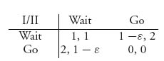
3.6 Choosing Among Several Nash Equilibria (Optional)
The concept of a Nash equilibrium is the most widely used idea of equilibrium in most fields, certainly in economics. But there is obviously a problem we have to deal with. How do we choose among the Nash equilibria in games where there are more than one? This must be addressed if we ever want to be able to predict the outcome of a game, which is, after all, the reason why we are studying this to begin with. But we have to warn the reader that many different criteria are used to choose a Nash equilibrium and there is no definitive way to make a choice.
The first idea is to use some sort of stability. Intuitively that means that we start with any strategy, say, for player II. Then we calculate the best response strategy for player I to this first strategy, then we calculate the best response strategy for player II to the best response for player I, and so on. There are many different things that could happen with this procedure. Here is our example.
Example 3.18 Let’s carry out the repeated best response idea for the two-person zero sum game
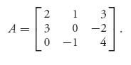
Note that v+ = v− = 1 and we have a saddle point at X* = (1, 0, 0), Y* = (0, 1, 0). Suppose that we start with a strategy for player II, Y0 = (0, 0, 1), so player II starts by playing column 3. The table summarizes the sequence of best responses:
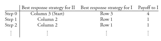
The best response to player II by player I is to play row 3 (and receive 4). The best response to that by player II is to play column 2 (and II receives −1). The best response to II’s choice of column 2 is now to play row 1 (and I receives 1). The best response of player II to player I’s choice of row 1 is to play column 2, and that is the end. We have arrived at the one and only saddle point of the matrix, namely, I plays row 1 and II plays column 2.
Similarly, you can check that this convergence to the saddle point will happen no matter where we start with a strategy, and no matter who chooses first. This is a really stable saddle point. Maybe it is because it is the only saddle point?
Nope. That isn’t the thing going on, because here is a matrix with only one saddle but the best response sequence doesn’t converge to it:
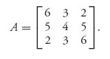
The value of this game is v(A) = 4, and there is a unique saddle at row 2 column 2. Now suppose that the players play as in the following table:
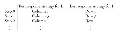
This just cycles from corner payoff to corner payoff and doesn’t get to the saddle. Only starting with row 2 or column 2 would bring us to the saddle, and that after only one step.
Stability seems to be a desirable characteristic for saddles and also for Nash points, especially with games that will be played many times. The next example considers a sort of stability to determine the choice of a Nash equilibrium among several candidates.
Example 3.19 Let’s consider the bimatrix game
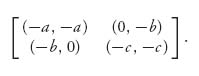
Assume a > b, c > 0. Because the game is symmetric with respect to payoffs, it doesn’t matter whether we talk about the row or column player. Then we have two pure Nash equilibria at (−b, 0) and at (0, −b). By calculating
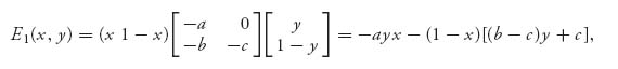
we see that setting
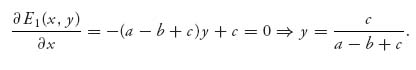
Similarly, ![]() . Defining
. Defining ![]() , we see that we also have a mixed Nash equilibrium at X = (h, 1 − h) = Y. Here is the table of payoffs for each of the three equilibria:
, we see that we also have a mixed Nash equilibrium at X = (h, 1 − h) = Y. Here is the table of payoffs for each of the three equilibria:
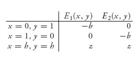
where z = E1(h, h) = −h2(a − b + c) − h(b − 2c) −c. To be concrete, suppose a = 3, b = 1, c = 2. Then h = ![]() gives the mixed Nash equilibrium X = Y = (
gives the mixed Nash equilibrium X = Y = (![]() ,
, ![]() ). These are the payoffs:
). These are the payoffs:
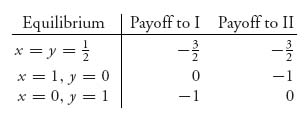
Now suppose that we go through a thought experiment. Both players are trying to maximize their own payoffs without knowing what the opponent will do. Player I sees that choosing x = 1 will do that, but only if II chooses y = 0. Player II sees that choosing y = 1 will maximize her payoff, but only if I chooses x = 0. Without knowing the opponent’s choice, they will end up playing (x = 1, y = 1), resulting in the nonoptimal payoff E1(1, 1) = −3 = E2(1, 1).
If there are many players playing this game whenever two players encounter each other and they each play nonoptimally, namely, x = 1, y = 1, they will all receive less than they could otherwise get. Eventually, one of the players will realize that everyone else is playing nonoptimally (x = 1) and decide to switch to playing x = 0 for player I, or y = 0 for player II. Knowing, or believing, that in the next game a player will be using y = 1, then player I can switch and use x = 0, receiving −1, instead of −3.
Now we are at an equilibrium x = 0, y = 1. But there is nothing to prevent other players from reaching this conclusion as well. Consequently others also start playing x = 0 or y = 0, and now we move again to the nonoptimal play x = 0, y = 0, resulting in payoffs −2 to each player.
If this reasoning is correct, then we could cycle forever between (x = 1, y = 1) and (x = 0, y = 0), until someone stumbles on trying x = h = ![]() . If player I uses x =
. If player I uses x = ![]() and everyone else is playing y = 0, then player I gets E1(
and everyone else is playing y = 0, then player I gets E1(![]() , 0) = −1 and player II gets E2(
, 0) = −1 and player II gets E2(![]() , 0) = −
, 0) = −![]() . Eventually, everyone will see that
. Eventually, everyone will see that ![]() is a better response to 0 and everyone will switch to h =
is a better response to 0 and everyone will switch to h = ![]() , that is, half the time playing the first row (or column) and half the time playing the second row (or column), When that happens, everyone receives −
, that is, half the time playing the first row (or column) and half the time playing the second row (or column), When that happens, everyone receives −![]() .
.
In addition, note that since E1(x, ![]() ) = E2(
) = E2(![]() , y) = −
, y) = −![]() for any x, y, no strategy chosen by either player can get a higher payoff if the opposing player chooses h =
for any x, y, no strategy chosen by either player can get a higher payoff if the opposing player chooses h = ![]() . That means that once a player hits on using x =
. That means that once a player hits on using x = ![]() or y =
or y = ![]() the cycling is over. No one can do better with a unilateral switch to something else, and there is no incentive to move to another equilibrium.
the cycling is over. No one can do better with a unilateral switch to something else, and there is no incentive to move to another equilibrium.
This Nash equilibrium x = y = ![]() is the only one that allows the players to choose without knowing the other’s choice and then have no incentive to do something else. It is stable in that sense.
is the only one that allows the players to choose without knowing the other’s choice and then have no incentive to do something else. It is stable in that sense.
This strategy is called uninvadable, or an evolutionary stable strategy, and shows us, sometimes, one way to pick the right Nash equilibrium when there are more than one. We will discuss this in much more depth when we discuss evolutionary stable strategies and population games in Chapter 7.
Stability is one criterion for picking a good Nash equilibrium, but there are others. Another criterion taking into account the idea of risk is discussed with an example.
Example 3.20 Entry Deterrence. There are two players producing gadgets. Firm (player) A is already producing and selling the gadgets, while firm (player) B is thinking of producing and selling the gadgets and competing with firm A. Firm A has two strategies: (1) join with firm B to control the total market (perhaps by setting prices), or (2) resist firm B and make it less profitable or unprofitable for firm B to enter the market (perhaps by lowering prices unilaterally). Firm B has the two strategies. (1) enter the market and compete with firm A, or (2) move on to something else. Here is the bimatrix:
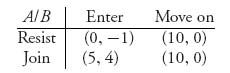
The idea is that a war hurts both sides, but sharing the market means less for firm A. There are two pure Nash equilibria:
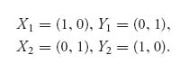
The associated payoffs for these Nash equilibria are
![]()
Assuming that firm B actually will make the first move, if firm B decides to enter the market, firm A will get 0 if A resists, but 5 if firm A joins with firm B. If firm B decides to not enter the market, then firm A gets 10. So, we consider the two Nash points (resist, move on) and (join, enter) in which the second Nash point gives firm A significantly less (5 vs. 10). So long as firm B does not enter the market, firm A can use either resist or join, but with any chance that firm B enters the market, firm A definitely prefers to join.
If firm B moves first, the best choice is Y2, which will yield it B2 (if A uses X2). Since B doesn’t know what A will do, suppose that B just chooses Y2 in the hope that A will use X2. Now, firm A looks over the payoffs and sees that X1 gives A a payoff of 10 (if B plays Y1). So the best for firm A is X1, which is resist. So, if each player plays the best for themselves without regard to what the other player will do, they will play X = (1, 0), Y = (1, 0) with the result that A gets 0 and B gets −1. This is the worst outcome for both players. Now, what?
In the previous example, we did not account for the fact that if there is any positive probability that player B will enter the market, then firm A must take this into account in order to reduce the risk. From this perspective, firm A would definitely not play resist because if Y* = (![]() , 1 −
, 1 − ![]() ), with
), with ![]() > 0 a very small number, then firm A is better off playing join. Economists say that equilibrium X2, Y2 risk dominates the other equilibrium and so that is the correct one. A risk-dominant Nash equilibrium will be correct the more uncertainty exists on the part of the players as to which strategy an opponent will choose; that is, the more risk and uncertainty, the more likely the risk-dominant Nash equilibrium will be played.
> 0 a very small number, then firm A is better off playing join. Economists say that equilibrium X2, Y2 risk dominates the other equilibrium and so that is the correct one. A risk-dominant Nash equilibrium will be correct the more uncertainty exists on the part of the players as to which strategy an opponent will choose; that is, the more risk and uncertainty, the more likely the risk-dominant Nash equilibrium will be played.
Finally, we end this section with a definition and discussion of Pareto-optimality. Pareto-optimality is yet another criterion used to choose among several Nash equilibria. Here is the definition and we will use this again later in the book.
Definition 3.6.1 Given a collection of payoff functions
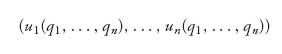
for an n-person nonzero sum game, where the qi is a pure or mixed strategy for player i = 1, 2, …, n, we say that ![]() is Pareto-optimal if there does not exist any other strategy for any of the players that makes that player better off, that is, increases her or his payoff, without making other players worse off, namely, decreasing at least one other player’s payoff.
is Pareto-optimal if there does not exist any other strategy for any of the players that makes that player better off, that is, increases her or his payoff, without making other players worse off, namely, decreasing at least one other player’s payoff.
From this perspective, it is clear that (5, 4) is the Pareto-optimal payoff point for the firms in entry deterrence because if either player deviates from using X2, Y2, then at least one of the two players does worse. On the other hand, if we look back at the prisoner’s dilemma problem at the beginning of this chapter we showed that (−5, −5) is a Nash equilibrium, but it is not Pareto-optimal because (−1, −1) simultaneously improves both their payoffs.
Closely related to Pareto-optimality is the concept of a payoff-dominant Nash equilibrium, which was introduced by Nobel Prize winners Harsanyi and Selten.
Definition 3.6.2 A Nash equilibrium is payoff-dominant if it is Pareto-optimal compared to all other Nash equilibria in the game.
Naturally, risk-dominant and payoff-dominant are two different things. Here is an example, commonly known as the stag-hunt game:
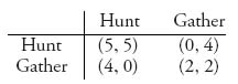
This is an example of a coordination game. The idea is that if the players can coordinate their actions and hunt, then they can both do better. Gathering alone is preferred to gathering together, but hunting alone is much worse than gathering alone.
The pure Nash equilibria are (hunt, hunt) and (gather, gather). There is also a mixed Nash equilibrium at X1 = (![]() ,
, ![]() ), Y1 = (
), Y1 = (![]() ,
, ![]() ). The following table summarizes the Nash points and their payoffs:
). The following table summarizes the Nash points and their payoffs:
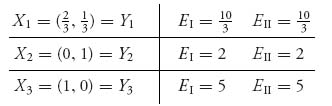
The Nash equilibrium X3, Y3 is payoff dominant because no player can do better no matter what. But the Nash equilibrium X2, Y2 risk dominates X3, Y3 (i.e., (gather, gather) risk dominates (hunt, hunt), The intuitive reasoning is that if either player is not absolutely certain that the other player will join the hunt, then the player who was going to hunt sees that she can do better by gathering. The result is that both players end up playing gather in order to minimize the risk of getting zero. Even though they both do worse, (gather, gather) is risk dominant. Note the resemblance to the prisoner’s dilemma game in which both players choose to confess because that is the risk-dominant strategy.
Problems
3.45 In the following games solved earlier, determine which, if any, Nash equilibrium is payoff dominant, risk dominant, and Pareto-optimal.
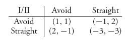
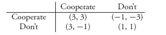
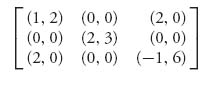
3.6.1 MAPLE/MATHEMATICA
Interior Nash Equilibrium. Maple can be used to solve the system of equations giving an interior Nash point. The commands for solving the preceding example are shown here:
> restart:with(LinearAlgebra):
> A:=Matrix([[-2, 5, 1], [-3, 2, 3], [2, 1, 3]]);
> B:=Matrix([[-4, -2, 4], [-3, 1, 4], [3, 1, -1]]);
> Y:=Vector(3, symbol=y):
> X:=Vector(3, symbol=x):
> yeq:=seq(add(y[j]*(A[i, j]-A[3, j]), j=1..3), i=1..2);
> xeq:=seq(add(x[i]*(B[i, s]-B[i, 3]), i=1..3), s=1..2);
> xsols:=solve({xeq[1] = 0, xeq[2] = 0, add(x[i], i=1..3)=1},
                               [x[1], x[2], x[3]]);
> assign(xsols);
> ysols:=solve({yeq[1] = 0, yeq[2] = 0, add(y[j], j=1..3)=1},
                               [y[1], y[2], y[3]]);
> assign(ysols);
> Transpose(X).A.Y; Transpose(X).B.Y;
The last line gives the expected payoffs to each player. The assign command assigns the solutions to the vectors. Observe too that when we calculate in Maple Transpose(X).A.Y the expected payoff to player I, the transpose appears to be on the wrong vector. But in Maple, vectors are defined as column matrices, so a correct multiplication is as is shown in the Maple commands, even though in the book we use XAYT.
If you change some of the numbers in the matrices A, B and rerun the Maple code, you will see that frequently the solutions will have negative components or the components will be greater than one. You have to be careful in trying to do this with Maple because solving the system of equations doesn’t always work, especially if there is more than one interior Nash equilibrium (which could occur for matrices that have more than two pure strategies).
3.6.2 MATHEMATICA FOR LEMKE–HOWSON ALGORITHM
This program will calculate Nash equilibria using the Lemke–Howson Algorithm. It automatically adjusts the starting positions to try to find as many Nash equilibria as possible.
FindNE2[matrixA_, matrixB_, iterations_] :=
 Module[{A = matrixA, B = matrixB, iter = iterations, xi, yj, obj,
   constr1, constr2, i, boundsA, boundsB, resultList, strats},
  If[Dimensions[A] != Dimensions[B],
   Print["Dimensions of A and B must match."]; Return[];, {}];
  Clear[x, y, p, q];
  (*Produce symbolic Subscript[x, i] and Subscript[y, j] variables*)
  xi = Table[Subscript[x, i], {i, 1, Dimensions[A][[1]]}];
  yj = Table[Subscript[y, i], {i, 1, Dimensions[A][[2]]}];
  (*Calculate objective function*)
  obj = Flatten[{xi}.A.Transpose[{yj}] + xi.B.Transpose[{yj}] -
    p - q];
  (*Get primary constraints*)
  constr1 = Map[# <= p &, Flatten[A.Transpose[{yj}]]];
  constr2 = Map[# <= q &, Flatten[{xi}.B]];
  resultList = {};
  (*VBounds gives an interval of the form [v^-,
  max entry of matrix]*)
  (*We know that for any NE p,
  q must reside in the intervals given by VBounds produced from A and B^T respectively*)
  boundsA = VBounds[A];
  boundsB = VBounds[Transpose[B]];
  For[i = 0, i < iter, i++,
   (*Build a list of solutions*)
   (*Here we produce random starting points for p and q instead of xi’s and yj’s*)
   AppendTo[resultList,
    FindMaximum[
      Join[obj, constr1, constr2, {Total[xi] == 1}, {Total[yj] == 1},
        Map[# >= 0 &, xi], Map[# >= 0 &, yj]],
      Join[xi,
        yj, {{p, RandomReal[boundsA]}}, {{q, RandomReal[boundsB]}}]]];
   ];
   (*Uncomment "TableForm[resultList]" and comment out last two lines  to see raw output*)
   (*TableForm[resultList]*)
   strats =
    FormatStrats[resultList, Dimensions[A][[1]], Dimensions[A][[2]]];
   {MatrixForm [strats[[1]]], MatrixForm[strats[[2]]],
    MatrixForm[strats[[3]]], MatrixForm[strats[[4]]]}
   ];
(*This just makes numbers close to zero print as 0’s instead ofprinting something like 3.45*10^-9*)
FormatStrats[ResultList_, RowDim_, ColDim_] :=
   Module[{resultList = ResultList, rowDim = RowDim, colDim = ColDim,
     xi, yj, vals, xVals, yVals, pVals, qVals},
     vals = Map[#[[2]] &, resultList];
     xi = Table[Subscript[x, i], {i, 1, rowDim}];
     yj = Table[Subscript[y, i], {i, 1, colDim}];
     (*Get numeric lists of Subscript[x, i]’s, Subscript[y, j]’s, p,
     and q*)
     xVals = Map[xi /. # &, vals];
     yVals = Map[yj /. # &, vals];
     pVals = Map[p /. # &, vals];
     qVals = Map[q /. # &, vals];
     (*Make numbers within .00001 of zero equal to zero*)
     {Chop[xVals, .00001], Chop[yVals, .00001], Chop[pVals, .00001],
     Chop[qVals, .00001]}
     ];


(*Example*)
A = {{-1, 0, 0}, {2, 1, 0}, {0, 1, 1}};
B = {{1, 2, 2}, {1, -1, 0}, {0, 1, 2}};
FindNE2[A, B, 3]

Mathematica finds the NE X=(0, 2/3, 1/3), Y=(1/3, 0, 2/3), p=2/3, q=2/3 and
X = (0, 0, 1), Y = (0, 0, 1), p=1, q=2.
Bibliographic Notes
The example games considered in this chapter (prisoner’s dilemma, chicken, battle of sexes, hawk–dove, stag–hare, etc.) are representative examples of the general class of games of pure competition, or cooperation, and so on. Rational reaction is a standard concept appearing in all game theory texts (see Wang 1988; Mesterton-Gibbons 2000; Ferguson (2013), for example).
The proof of existence of a Nash equilibrium given here is due to Nash, but there are many proofs of this result that do not use the Kakutani fixed-point theorem and are considered more elementary. The nonlinear programming approach to the calculation of a Nash equilibrium originates with Lemke and Howson (1964). The main advantage of their approach is the fact that it combines two separate optimization problems over two sets of variables into one optimization problem over one set of variables; that is, instead of maximizing EI(X, Y) over X for fixed Y and EII(X, Y) over Y for fixed X, we maximize EI(X, Y) + EII(X, Y) − p − q over all variables (X, Y, p, q) at the same time. Computationally, this is much easier to carry out on a computer, which is the main advantage of the Lemke–Howson algorithm.
All the games of this chapter can be solved using the software package Gambit as a blackbox in which the matrices are entered and all the Nash equilibria as well as the expected payoffs are calculated.
1 See Appendix E for a short biography.
2 Israel has never admitted to having nuclear weapons, but it is widely accepted as true and reported as a fact. The secrecy on the part of the Israelis also indicates an implicit understanding of the bimatrix game here.
3 Alternatively we may take the partial derivative of the function with a Lagrange multiplier ![]() ). Taking a partial with respect to xk shows that
). Taking a partial with respect to xk shows that ![]() E1/
E1/![]() xk =
xk = ![]() E1/
E1/![]() xn for all k = 1, 2, …, n − 1. This gives us the same system as (3.1).
xn for all k = 1, 2, …, n − 1. This gives us the same system as (3.1).
4 Professor at Hebrew University and winner of the 2005 Nobel prize in economics.