Appendix C: The Essentials of Maple

In this appendix, we will review some of the basic Maple operations used in this book. Maple has a very helpful feature of providing context-sensitive help. That means that if you forget how a command is used, or even what the command is, simply type the word and click on it. Go to the Help menu, and you will see “Help on your word” which will give you the help available for that command.

Throughout this book we have used the worksheet mode of Maple version 10.0. The commands will work in version 10.0 or any later version. In 2012 version 16.04 is current.

C.1 Features

The major features of Maple are listed as follows:

C.1.1 OPERATORS, SIGNS, SYMBOLS, AND COMMANDS

The basic arithmetic operations are +, −, *, /, ⋀ for addition, subtraction, multiplication, division, and exponentiation, respectively. Any command must end with a semicolon “;” if you use a colon “:” instead, the statement will be executed but no output will appear. To clear all variables and definitions in a worksheet use restart:.

Parentheses (...) are used for algebraic grouping and arguments of functions just as they are in algebra. You cannot use braces or brackets for that! Braces {...} are used for sets, and brackets [...] for lists.

Multiplication uses an asterisk (e.g., x*y, not xy); exponents by a caret (e.g., x⋀2 = x2).

To make an assignment like a: =3*x+4, use := to assign 3 * x + 2 to the symbol a. The equation a=3*x+4 is made with the equal sign and not colon equal.

The percent sign (%) refers to the immediately preceding output; %% gives the next-to-last output, and so on.

The command unapply converts a mathematical expression into a function. For example, if you type the command g :=unapply (3*x+4*z, [x, z]) this converts 3x + 4z into the function g(x, z) = 3x + 4z.

C.2 Functions

A direct way of defining a function is by using

For example,

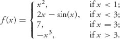
defines A piecewise defined function is entered using the command piecewise. For example,

defines

C.2.1 DERIVATIVES AND INTEGRALS OF FUNCTIONS

The derivative of a function with respect to a variable is obtained by

to get ∂f(x, y)/∂y. Second derivatives simply repeat the variable:

is ∂2 f /∂ y2.

To get an integral, use

to obtain Use

for If Maple cannot get an exact answer, you may use

to evaluate it numerically.

Whenever you get an expression that is complicated, use simplify(%) to simplify it. If you want the expression expanded, use expand(%), or factored factor(%).

C.2.2 PLOTTING FUNCTIONS

Maple has a very powerful graphing capability. The full range of plotting capabilities is accessed by using the command with(plots): and with(plottools):. To get a straightforward plot of the function f(x), use

or, for a three-dimensional (3d) plot.

There are many options for the display of the plots which can be accessed by typing ?plot/options.

To plot more than one curve on the same graph, use

fplot:=plot(f(x), x=a..b):
gplot:=plot(g(x), x=c..d):
display(fplot, gplot);

C.2.3 MATRICES AND VECTORS

A matrix is entered by first loading the set of Maple commands dealing with linear algebra: with(LinearAlgebra): and then using

It is a list of lists. Individual elements of A are obtained using A[i, j].

The commands to manipulate matrices are as follows:

• A+B or MatrixAdd (A, B) adds element by element aij + bij.
• c*A gives c aij.
• A.B is the product of A and B assuming that the number of rows of B is the same as the number of columns of A.
• Transpose(A) gives AT.
• Either Inverse(A) or simply A⋀(-1) gives A−1 for a square matrix which has an inverse, and can be checked by calculating Determinant(A).
• ConstantMatrix(-1, 3, 3) defines a 3 × 3 matrix in which each element is −1.

Suppose now that A is a 3 × 3 matrix. If you define a vector in Maple by X :=<x1, x2, x3>, Maple writes this as a 3 × 1 column matrix. So both Transpose(X).A and A.X are defined. You can always find the dimensions of a matrix using RowDimension(A) and ColDimension(A).

C.3 Some Commands Used in This Book

We will briefly describe the use of some specialized commands used throughout the book.

1. Given a game with matrix A, the upper value v+ and lower value v− are calculated with the respective commands

and

The command seq(A[i, j], i=1..rows) considers for each fixed jth column each element of the ith row of the matrix A. Then max(seq) finds the largest of those.

2. To solve a system of equations, we use

eqs:=y1+2*y2+3*y3-v=0, 3*y1+y2+2*y3-v=0, 
             2*y1+3*y2+y3-v=0, y1+y2+y3-1=0;
solve(eqs, [y1, y2, y3, v]);

Define the set of equations using {...} and solve for the list of variables using [...].

3. To invoke the simplex method and solve a linear programming problem load, the package with(simplex): and then the command

minimizes the objective function, subject to the constraints, along with the constraint that the variables must be nonnegative. This returns exact solutions if there are any. You may also use the Optimization package, which picks the best method to solve: with(Optimization) loads the package, and then the command

Minimize (obj, cnsts, assume=nonnegative) ;

solves the problem.

4. The Optimization package is used to solve nonlinear programming problems as well. In game theory, the problems can be solved using either QPSolve, which solves quadratic programming problems, or NLPSolve, which numerically solves general nonlinear programs. For example, we have used either the command

QPSolve(objective, Cnst, assume=nonnegative, maximize, 
                            initialpoint=(q=1, p=2));

or the command

NLPSolve(objective, Cnst, assume=nonnegative, maximize);

to solve problems. The search for additional solutions can be performed by setting the variable initialpoint.

5. To substitute a specific value into a variable, use the command

We use this in several places, one of which is in evaluating the core of a cooperative game. For example,

cnsts:=-x1<=z, -x2<=z, -(5/2-x1-x2)<=z, 2-x1-x2<=z, 
                    1-x2-(5/2-x1-x2)<=z, -x1-(5/2-x1-x2)<=z;
Core:=subs(z=0, cnsts);

gives

6. A region in the plane defined by inequalities are plotted using the command

> with(plots):
> inequal(Core, x1=0..2, x2=0..3, 
              optionsfeasible=(color=red), 
              optionsopen=(color=blue, thickness=2), 
              optionsclosed=(color=green, thickness=3), 
              optionsexcluded=(color=yellow));

The region Core is plotted. The set of points that satisfy the inequalities are in red, and the set of points that violate at least one inequality are colored yellow. The boundary of the feasible set is drawn in different colors depending on whether the inequality is strict or not. Strict inequalities are blue, and closed inequalities are drawn green.

7. A system of linear inequalities may be solved, actually reduced, to a minimal set of inequalities using the package with(SolveTools:-Inequality). For example,

> with(SolveTools:-Inequality):
> cnsts:=x+y<=1, y>=3*x-20, x<=3/4, y>=-1, x>=0;
> glc:=LinearMultivariateSystem(cnsts, [x, y]);

gives the output

8. To plot a polygon connecting a list of points, we use

> with(plottools):
> pure:=([[2, 1], [-1, -1], [-1, -1], [1, 2]]);
> pp:=pointplot(pure);
> pq:=polygon(pure, color=yellow);
> display(pp, pq)

This plots the points pure and the polygon with the points as the vertices, and then colors the interior of the polygon yellow. To plot a sequence of points generated from two functions first define the points using

> points:=seq(seq([f(x, y), g(x, y)], x=0..1, 0.05), y=0..1, 0.05):

This is on the square (x, y) [0, 1] × [0, 1] with step size 0.05 for each variable. This produces 400 points (20 x values and 20 y values). Note the colon at the end of this command, which suppresses the actual display of all 400 points. Then pointplot(points); produces the plot.

9. In order to plot the solution of a system of ordinary differential equations we need the package with(DEtools) and with(plots). For instance, consider the commands

> ode:={D(p1)(t)=p1(t)*(p2(t)-p3(t)), 
       D(p2)(t)=p2(t)*(-p1(t)+p3(t)), 
       D(p3)(t)=p3(t)*(p1(t)-p2(t))};
> subs(p3=1-p1-p2, ode);
> G:=simplify(%);

> DEplot3d(G[1], G[2], p1(t), p2(t), t=0..20, 
           [[p1(0)=0.1, p2(0)=0.2], [p1(0)=0.6, 
                      p2(0)=.2], [p1(0)=1/3, p2(0)=1/3]], 
           scene=[t, p1(t), p2(t)], 
           stepsize=.1, linecolor=t, 
           title=”Cycle around the steady state”);

The first statement assigns the system of differential equations to the set named ode. The subs command substitutes p3=1-p1-p2 in the set ode. G:=simplfy(%) puts the result of simplifying the previous substitution into G. There are now exactly two equations into the set G and they are assigned to G[1] and G[2]. The DEplot3d command numerically solves the system {G[1], G[2]} for the functions [p1(t), p2(t)] on the interval 0 ≤ t ≤ 20 and plots the resulting curves starting from the different initial points listed in three dimensions.