Appendix D: The Mathematica Commands

In this appendix, we will translate the primary Maple commands we used throughout the book to Mathematica version 5.2. Any later version of Mathematica will work in the same way.

D.1 The Upper and Lower Values of a Game

We begin by showing how to use Mathematica to calculate the lower value

and the upper value

of the matrix A.

Enter the matrix

A={{1, 4, 7}, {-1, 3, 5}, {2, -6, 1.4}}
rows = Dimensions[A][[1]]
      cols = Dimensions[A][[2]]
        a = Table[Min[A[[i]]], {i, rows}]
          b = Max[a[[]]]
            Print["The lower value of the game is= ", b]
            c = Table[Max[A[[All, j]]], {j, cols}]
              d = Min["c[[]]]
              Print["The upper value is=", d]

These commands will give the upper and lower values of A. Observe that we do not need to load any packages and we do not need to end a statement with a semicolon. On the other hand, to execute a statement we need to push Shift + Enter at the same time.

D.2 The Value of an Invertible Matrix Game with Mixed Strategies

The value and optimal strategies of a game with an invertible matrix (or one which can be made invertible by adding a constant) are calculated in the following. The formulas we use are as follows:

and

If these are legitimate strategies, then the whole procedure works; that is, the procedure is actually calculating the saddle point and the value:

A = {{4, 2, -1}, {-4, 1, 4}, {0, -1, 5}}
         {{4, 2, -1}, {-4, 1, 4}, {0, -1, 5}}
Det[A]
     72
A1 = A + 3
     {{7, 5, 2}, {-1, 4, 7}, {3, 2, 8}}
B=Inverse[A1]
     {{2/27, -4/27, 1/9}, {29/243, 50/243, -17/81}, 
      {-14/243, 1/243, 11/81}}
J= {1, 1, 1}
     {1, 1, 1}
v = 1/J.B.J
     81/19
X =v*(J.B)
     {11/19, 5/19, 3/19}
Y = v*(B.J)
     {3/19, 28/57, 20/57}

At the end of each statement, having pushed shift+enter, we are showing the Mathematica result. Remember that you have to subtract the constant you added to the matrix at the beginning in order to get the value for the original matrix. So the actual value of the game is

D.3 Solving Matrix Games by Linear Programming

In this subsection, we present the use of Mathematica to solve a game using the two methods of using linear programming

Method 1. The Mathematica command

LinearProgramming[c, m, b]

finds a vector x that minimizes the quantity c .x subject to the constraints m.x ≥ b, x ≥ 0, where m is a matrix and b is a vector. This is the easiest way to solve the game.

Recall that for the matrix

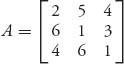
player I’s problem becomes

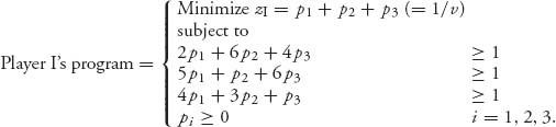
After finding the pi values, we will set

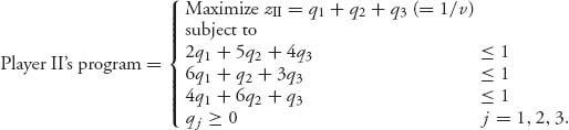
Then xi = vpi will give the optimal strategy for player I. Player II’s problem is

The Mathematica solution of these is given as follows:

The matrix is:
A={{2, 5, 4}, {6, 1, 3}, {4, 6, 1}}
c={1, 1, 1}
b={1, 1, 1}
 
PlayI=LinearProgramming[c, Transpose[A], b]
      {21/124, 13/124, 1/124}
PlayII=LinearProgramming[-b, A, {{1, -1}, {1, -1}, {1, -1}}]
      {13/124, 10/124, 12/124}
v=1/(21/124+13/124+1/124)
124/35
 
Y=v*PlayII
{13/35, 10/35, 12/35}
 
X=v*PlayI
{21/35, 13/35, 1/35}

The value of the original game is In PlayII, the constraints must be of the form ≤. The way to get that in Mathematica is to make each constraint a pair where the second number is either 0, if the constraint is equality =; it is −1, if the constraint is ≤; and 1, if the constraint is ≥. The default is 1 and that is why we don’t need the pair in PlayI.

It is also possible and sometimes preferable to use the Mathematica function Minimize, or Maximize. For this problem the commands become:

For player I,

Minimize[{x + y + z, 2x + 6y + 4z >= 1, 5x + y + 6z >= 1, 
             4x + 3y + z >= 1, x>=0, y>=0, z>=0}, {x, y, z}]
   {35/124, {x->21/124, y->13/124, z->1/124}}

For player II,

Maximize[{x + y + z, 2x + 5y + 4z <= 1, 
                     6x + y + 3z <= 1, 4x + 6y + z <= 1, 
                     x >= 0, y >= 0, z >= 0}, {x, y, z}]
 
   {35/124, {x->13/124, y->5/62, z->3/31}}

You may also use these commands with matrices and vectors.

Method 2. Player II’s problem is

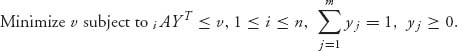
Player I’s problem is

For example, if we start with the game matrix

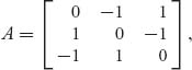
we may solve player I’s problem using the Mathematica command

Maximize[{v, y - z >= v, -x + z >= v, x - 
             y >= v, x + y + z == 1, 
             x >= 0, y >= 0, z >=0}, {x, y, z, v}]

This gives the output Similarly, you can use Minimize to solve player II’s program.

We may also use the LinearProgramming function in matrix form, but now it becomes more complicated because we have an equality constraint as well as the additional variable v.

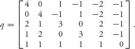
Here is an example. Take the Colonel Blotto game

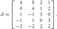
The Mathematica command

solves the following program: Minimize c · x subject to mx ≥ b, x ≥ 0. To use this command for player II, our coefficient variables are c = (0, 0, 0, 0, 1) for the objective function zII = 0y1 + 0y2 + 0y3 + 0y4 + 1v. The matrix m is

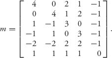
The last column is added for the variable v. The last row is added for the constraint y1 + y2 + y3 + y4 = 1. Finally, the vector b becomes

The first number, 0, is the actual constraint, and the second number makes the inequality ≤ instead of the default ≥. The pair {1, 0} in b comes from the equality constraint y1 + y2 + y3 + y4 = 1 and the second zero converts the inequality to equality. So here it is

m = {{4, 0, 2, 1, -1}, {0, 4, 1, 2, -1}, {1, -1, 3, 0, -1}, 
    {-1, 1, 0, 3, -1}, {-2, -2, 2, 2, -1}, {1, 1, 1, 1, 0}}
c = {0, 0, 0, 0, 1}
b = {{0, -1}, {0, -1}, {0, -1}, {0, -1}, {0, -1}, {1, 0}}
LinearProgramming[c, m, b]

Mathematica gives the output

The solution for player I is found similarly, but we have to be careful because we have to put it into the form for the LinearProgramming command in Mathematica, which always minimizes and the constraints in Mathematica form are ≥. Player I’s problem is a maximization problem so the cost vector is

corresponding to the variables x1, x2, …, x5, and −v. The constraint matrix is the transpose of the Blotto matrix but with a row added for the constraint x1 + ··· + x5 = 1. It becomes

Finally, the b vector becomes

In each pair, the second number 1 means that the inequalities are of the form ≥. In the last pair, the second 0 means the inequality is actually = . For instance, the first and last constraints are, respectively,

With this setup the Mathematica command to solve is simply

with output

D.4 Interior Nash Points

The system of equations for an interior mixed Nash equilibrium are given by

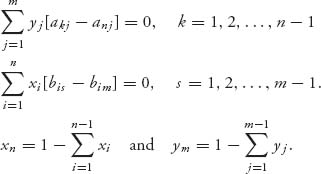
The game has matrices (A, B) and the equations, if they have a solution that are strategies, will yield X* = (x1, …, xn) and Y* = (y1, …, ym).

The following example shows how to set up and solve using Mathematica:

A = {{-2, 5, 1}, {-3, 2, 3}, {2, 1, 3}}
B = {{-4, -2, 4}, {-3, 1, 4}, {3, 1, -1}}
rowdim = Dimensions[A][[1]]
coldim = Dimensions[B][[2]]
Y = Array[y, coldim]
X= Array[x, rowdim]
EQ1 = Table[Sum[y[j](A[[k, j]]-A[[rowdim, j]]), 
               {j, coldim}], {k, rowdim-1}]
EQ2 = Table[Sum[x[i](B[[i, s]]-B[[i, coldim]]), 
               {i, rowdim}], {s, coldim-1}]
Solve[{EQ1[[1]] == 0, EQ1[[2]] == 0, y[1] + y[2] + y[3] == 1}, 
             {y[1], y[2], y[3]}]
Solve[{EQ2[[1]] == 0, EQ2[[2]] == 0, x[1] + x[2] + x[3] == 1}, 
             {x[1], x[2], x[3]}]

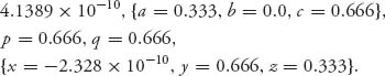
Mathematica gives the output

D.5 Lemke–Howson Algorithm for Nash Equilibrium

A Nash equilibrium of a bimatrix game with matrices (A, B) is found by solving the nonlinear programming problem

subject to

Here is the use of Mathematica to solve for a particular example:

A = {{-1, 0, 0}, {2, 1, 0}, {0, 1, 1}}
B = {{1, 2, 2}, {1, -1, 0}, {0, 1, 2}}
f[X_] = X.B
g[Y_] = A.Y
NMaximize[{f[{x, y, z}].{a, b, c} + {x, y, z}.g[{a, b, c}] - p - q, 
 f[{x, y, z}][[1]] - q <= 0, 
 f[{x, y, z}][[2]] - q <= 0, f[{x, y, z}][[3]] - q <= 0, 
 g[{a, b, c}][[1]] - p <= 0, g[{a, b, c}][[2]] - p <= 0, 
 g[{a, b, c}][[3]] - p <= 0, x + y + z == 1, x >= 0, y >= 0, z >= 0, 
 a >= 0, b >= 0, c >= 0, a + b + c == 1}, {x, y, z, a, b, c, p, q}]

The command NMaximize will seek a maximum numerically rather than symbolically. This is the preferred method for solving using the Lemke–Howson algorithm because of the difficulty of solving optimization problems with constraints. This command produces the Mathematica output

The first number verifies that the maximum of f is indeed zero. The optimal strategies for each player are The expected payoff to player I is and the expected payoff to player II is

D.6 Is the Core Empty?

A simple check to determine if the core is empty uses a simple linear program. The core is

Convert to a linear program

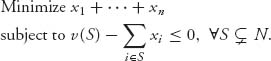
If the solution of this program produces a minimum of x1 + ··· + xn >v(N), we know that the core is empty; otherwise it is not. For example, if N = {1, 2, 3}, and

we may use the Mathematica command

Minimize[{x1+x2+x3, x1+x2>=105, x1+x3>=120, 
          x2+x3>=135, x1>=0, x2>=2}, {x1, x2, x3}].

Mathematica tells us that the minimum of x1 + x2 + x3 is 180 > v(123) = 150. So C(0) = . The other way to see this is with the Mathematica command

LinearProgramming[{1, 1, 1}, {{1, 1, 0}, {1, 0, 1}, 
                              {0, 1, 1}}, {105, 120, 135}]

which gives the output {x1 = 45, x2 = 60, x3 = 75} and minimum 180. The vector c = (1, 1, 1) is the coefficient vector of the objective c · (x1, x2, x3); the matrix

is the matrix of constraints of the form ≥ b; and b = (105, 120, 135) is the right-hand side of the constraints.

D.7 Find and Plot the Least Core

The ε-core is

You need to find the smallest ε1 for which C(ε1) ≠ .

For example, we use the characteristic function

v1 = 0; v2 = 0; v3 = 0;
v12 = 2; v13 = 0; v23 = 1; v123 = 5/2;

and then the Mathematica command

Minimize[{z, v1 - x1 <= z, v2 - x2 <= z, v3 - x3 <= z, 
         v12 - x1 - x2 <= z, v13 - x1 - x3 <= z, v23 - x2 - x3 <= z, 
         x1 + x2 + x3 == v123}, {z, x1, x2, x3}]

This gives the output

The important quantity is because we do not know yet whether C(ε1) contains only one point. At this stage, we know that and if we take any then C(ε) = .

Here is how you find the least core and get a plot of C(0) in Mathematica:

Core[z]:= {v1 - x1 <= z, v2 - x2 <= z, v3 - x3 <= z, 
           v12 - x1 - x2 <= z, v13 - x1 - x3 <= z, 
           v23 - x2 - x3 <= z, x1 + x2 + x3 == v123}
 
A[z]:= {z, Core[z]} Minimize[A[z], {z, x1, x2, x3}]
 
Output:-1/4, {z -> -1/4, x1 -> 5/4, x2 -> 1, x3 -> 1/4}
 
S = Simplify[Core[z] /. {z -> 0, x3 -> v123 - x1 - x2}]
      Substitute z=0, x3=v123-x1-x2 in C[z]
<< Algebra'InequalitySolve'
      Load the InequalitySolve package
 
<< Graphics'InequalityGraphics'
      Load the InequalityGraphics package.
 
InequalitySolve[S, {x1, x2}]
      Output: 0 <= x1 <= 3/2 && 2 - x1 <= x2 <= 1/2(5 - 2 x1)
      Solve inequalities in C[0] to see if one point.
 
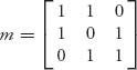
InequalityPlot[S, {x1, -2, 2}, {x2, -2, 2}]
      Plot the core C[0] (see below)
 
F = Simplify[Core[z] /. {z -> -1/4, x3 -> v123 - x1 - x2}]
      Substitute z=-1/4 for least core.
 
InequalitySolve[F, {x1, x2}]
 
      Output: 1/4 <= x1 <= 5/4 && x2 == 1/4(9 - 4 x1)
      Solve inequalities in C[-1/4] to see if one point.
 
Plot[(9 - 4 x1)/4, {x1, 1/4, 5/4}]
      C[-1/4] is a line segment.

Here is C(0) for the example, generated with Mathematica:

D.8 Nucleolus and Shapley Value Procedure

This section will give the Mathematica procedure to find the nucleolus and the Shapley Value. The nucleolus and Shapley value procedure is presented as a three-player example. The Mathematica commands are interspersed with output and is self-documenting.

Clear the variables:
Clear[x1, x2, x3, v1, v2, v3, v12, v13, v23, v123, z, w, S, S2, A, Core]
Define the characteristic function:
v1=0;v2=0;v3=0;v12=1/3;v13=1/6;v23=5/6;v123=1;
 
Core[z]:={v1-x1<=z, v2-x2<=z, v3-x3<=z, v12-x1-x2<=z, 
          v13-x1-x3<=z, v23-x2-x3<=z, x1+x2+x3==v123}
 
A[z]:={z, Core[z]}
 
Minimize[A[z], {z, x1, x2, x3}]
 
Output:-1/12, {z=-1/12, x1=1/12, x2=1/3, x3=7/12}
 
S=Simplify[Core[z]/.{z->-1/12, x3->v123-x1-x2}]
 
<<Algebra'InequalitySolve'
<<Graphics'InequalityGraphics'
 
InequalitySolve[S, {x1, x2}]
 
Output:
x1=1/12 && 1/3<= x2 <= 3/4
 
Assign the known variables.
 
x1=1/12;z=-1/12;x3=v123-x1-x2
 
Now check the excesses to see which coalitions can be dropped:
 
v1-x1=-1/2
v2-x2=-x2
v3-x3=-11/12+x2
v12-x1-x2=1/4-x2
v13-x1-x3=-5/6+x2
v23-x2-x3=-1/12
 
We may drop coalitions {1} and {23} and then recalculate
 
B[w]={v2-x2<=w, v3-x3<=w, v12-x1-x2<=w, 
                     v13-x1-x3<=w, x1+x2+x3==v123}
 
Find the smallest w which makes B[w] nonempty
Minimize[{w, B[w]}, {x2, w}]
 
Output:-7/24, {x2 = 13/24, w = -7/24}
 
Check to see if we are done:
S2=Simplify[B[w]/.w->-7/24]
 
InequalitySolve[S2, {x2}]
 
Output:x2= 13/24
This is the end because we now know x1=1/12, x2=13/24, x3=9/24.

The final result gives the nucleolus as

The procedure to get the Shapley value is very simple:

S={1, 2, 3}
numPlayers=Length[S]
L=Subsets[S]
K=Length[L]
v[{1}]=25;
v[{2}]=40;
v[{3}]=0;
v[{1, 2}]=90;
v[{1, 3}]=35;
v[{2, 3}]=50;
v[{1, 2, 3}]=100;
v[{}]=0;
For[i=1, i<=numPlayers, i++, 
{x[i]=0;
For[k=1, k<=K, k++, 
If[MemberQ[L[[k]], i] && Length[L[[k]]]>=1, 
x[i]=x[i]+(v[L[[k]]]-v[DeleteCases[L[[k]], i]])*(Factorial[Length[L[[k]]]-
1]*Factorial[numPlayers-Length[L[[k]]]])/Factorial[numPlayers]]], Print
 [x[i]]}]

The output for this example is

x[1]=235/6, x[2]=325/6, x[3]=20/3.

D.9 Plotting the Payoff Pairs

Given a bimatrix game with matrices (A, B) that are each 2 × 2 matrices, the expected payoff to player I is

and for player II

We want to get an idea of the shape of the set of payoff pairs (EI(x, y), EII(x, y)). In Mathematica, we can do that with the following commands:

A = {{2, -1}, {-1, 1}}
B = {{1, -1}, {-1, 2}}
f[x_, y_] = {x, 1 - x}.A.{y, 1 - y}
g[x_, y_] = {x, 1 - x}.B.{y, 1 - y}
 
h[x_, y_] = {f[x, y], g[x, y]}
 
values = Table[Table[h[x, y], {x, 0, 1, .025}], {y, 0, 1, 0.025}];
 
s = Flatten[values, 1];
 
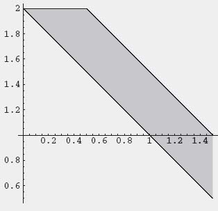
ListPlot[s]

Observe that a function is defined in Mathematica as, for example,

                                            f[x_, y_] = {x, 1 - x}.A.{y, 1 - y}, 

which gives EI(x, y). Mathematica uses the symbol x_ to indicate that x is a variable. The result of these commands is the following graph:

D.10 Bargaining Solutions

We will use Mathematica to solve the following bargaining problem with bimatrix:

First we use the safety point u* = value(A), v* = value(BT). Here are the commands to find (u*, v*):

The matrix is:
A={{1, -4/3}, {-3, 4}}
player I's problem is:
Maximize[{v, {x, y}.A[[All, 1]] >= v, {x, y}.A[[All, 2]] >= v, 
    x + y == 1, x >= 0, y >= 0}, {x, y, v}]
player II's problem is:
Minimize[{v, A[[1]].{x, y} <= v, A[[2]].{x, y} <= v, 
    x + y == 1, x >= 0, y >= 0}, {x, y, v}]

This finds u* = value(A) = 0, and, even though we don’t need it, For v* we use

B = {{4, -4}, {-1, 1}}
BT = Transpose[B]
Minimize[{v, BT[[1]].{x, y} <= v, BT[[2]].{x, y} <= v, 
   x + y == 1, x >= 0, y >= 0}, {x, y, v}]

which tells us that v* = value(BT) = 0 and

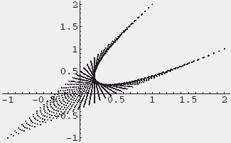
So our safety point is (u*, v*) = (0, 0). A plot of the feasible set is found from

ListPlot[{{1, 4}, {-3, -1}, {-4/3, -4}, {4, 1}, {1, 4}}, 
                                       PlotJoined -> True]

which produces

You can see that the Pareto-optimal boundary is the line through (4, 1) and (1, 4) which has the equation given by v − 1 = −(u − 4). So now the bargaining problem with safety point (0, 0) is

subject to the constraints

The Mathematica command is

Maximize[{u v, v <= -u + 5, v <= 5/4 u + 11/4, v >= -9/5 u - 32/5, 
    v >= 15/16 u - 11/16, u >= 0, v >= 0}, {u, v}]

and gives the output and the maximum is This is achieved if the two players agree to play and receive (1, 4) and (4, 1) exactly half the time. Then they each get

Next, we find the optimal threat strategies.

First, we have seen that the Pareto-optimal boundary is the line v = − u + 5, which has slope mp = −1. So we look at the game with matrix −mp A − B, or

It is the optimal strategies we need for this game. However, in this case it is easy to see that there is a pure saddle point Xt = (0, 1), Yt = (1, 0). Consequently, the threat safety point is

The Mathematica command to solve the bargaining problem with this safety point is

Maximize[{(u + 3) (v + 1), v <= -u + 5, v <= 5/4 u + 11/4, 
             v >= -9/5 u - 32/5, 
             v >= 15/16 u - 11/16, u >= -3, v >= -1}, {u, v}]

which gives the output and maximum In this solution, player I gets less and player II gets more to reflect the fact that player II has a credible and powerful threat. So the payoffs are obtained by each agreeing to receive (1, 4) exactly five-sixths of the time and payoff (4, 1) exactly one-sixth of the time (player I throws player II a bone once every 6 plays).

D.11 Mathematica for Replicator Dynamics

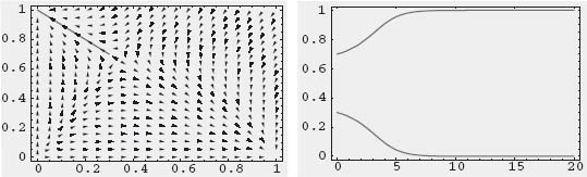
Naturally, the solution of the replicator dynamics equations (7.11) depends on the matrices involved so we will only give some sample Mathematica commands to produce graphs of the vector fields and trajectories.

For example,

Needs["Graphics'PlotField'"];
a = 2
b = 1
Here is the system we consider:
e1 = p1'[t] == p1[t] (a p1[t] - a p1[t]^2 - b p2[t]^2)
e2 = p2'[t] == p2[t] (b p2[t] - a p1[t]^2 - b p2[t]^2)
This command gives a plot of the vector field in the figure below:
field = PlotVectorField[{x (a x - a x^2 - b y^2), 
        y (b y - a x^2 - b y^2)}, {x, 0, 1, 0.25}, {y, 0, 1, 0.2}, 
        PlotPoints -> 20, Frame -> True];
 
This command solves the system for the initial point p1[0], p2[0]:
nsoln = NDSolve[{e1, e2, p1[0] == .3, 
                         p2[0] == .7}, {p1, p2}, {t, 0, 20}];
 
This plots the trajectory (p1[t], p2[t]) with p1 versus p2:
trajectory =
    ParametricPlot[{p1[t], p2[t]} /. nsoln[[1]], {t, 0, 20}, 
              PlotRange -> All, 
              PlotStyle -> {Hue[1]}, Frame -> True];
 
This command plots the trajectory superimposed on the vector field:
 
Show[trajectory, field];
 
If you want a graph of the individual functions use:
trajectory1 = ParametricPlot[{t, p1[t]} /. nsoln[[1]], 
                            {t, 0, 20}, PlotRange -> All, 
                            PlotStyle -> {Hue[1]}, Frame -> True];
  
trajectory2 = ParametricPlot[{t, p2[t]} /. nsoln[[1]], 
                            {t, 0, 20}, PlotRange -> All, 
                            PlotStyle -> {Hue[1]}, Frame -> True];
Show[trajectory1, trajectory2];

This last command produces the following plot of both functions on one graph: