
Appendix B: The Essentials of Probability
In this section, we give a brief review of the basic probability concepts and definitions used or alluded to in this book. For further information, there are many excellent books on probability (e.g., see the book by Ross, 2002).
The space of all possible outcomes of an experiment is labeled Ω. Events are subsets of the space of all possible outcomes, A ⊂ Ω. Given two events A, B, the event
The probability of an event A is written as P(A) or Prob(A). It must be true that for any event A, 0 ≤ P(A) ≤ 1. In addition,
Given two events A, B with P(B) > 0, the conditional probability of A given the event B has occurred, is defined by
![]()
Two events are therefore independent if and only if P(A | B) = P(A) so that the knowledge that B has occurred does not affect the probability of A. The very important laws of total probability are frequently used:
These give us a way to calculate the probability of A by breaking down cases. Using the formulas, if we want to calculate P(A| B) but know P(B|A) and P(B|Ac), we can use Bayes’ rule:
![]()
A random variable is a function X: ![]() that is, a real-valued function of outcomes of an experiment. As such, this random variable takes on its values by chance. We consider events of the form
that is, a real-valued function of outcomes of an experiment. As such, this random variable takes on its values by chance. We consider events of the form
{ω ![]() Ω: X(ω) ≤ x} for values of
Ω: X(ω) ≤ x} for values of ![]() For simplicity, this event is written as {X ≤ x} and the function
For simplicity, this event is written as {X ≤ x} and the function
![]()
is called the cumulative distribution function of X. We have
A random variable X is said to be discrete if there is a finite or countable set of numbers x1, x2, …, so that X takes on only these values with P(X = xi) = pi, where 0 ≤ pi ≤ 1, and ∑i pi = 1. The cumulative distribution function is a step function with a jump of size pi at each xi, ![]()
A random variable is said to be continuous if P(X = x) = 0 for every ![]() and the cumulative distribution function FX(x) = P(X ≤ x) is a continuous function. The probability that a continuous random variable is any particular value is always zero. A probability density function for X is a function
and the cumulative distribution function FX(x) = P(X ≤ x) is a continuous function. The probability that a continuous random variable is any particular value is always zero. A probability density function for X is a function
![]()
In addition, we have
![]()
The cumulative distribution up to x is the area under the density from −∞ to x. With an abuse of notation, we often see P(X = x) = fX(x), which is clearly nonsense, but it gets the idea across that the density at x is roughly the probability that X = x.
Two random variables X and Y are independent if P(X ≤ x and Y ≤ y) = P(X ≤ x)P(X ≤ y) for all ![]() If the densities exist, this is equivalent to f(x, y) = fX(x) fY(y), where f(x, y) is the joint density of (X, Y).
If the densities exist, this is equivalent to f(x, y) = fX(x) fY(y), where f(x, y) is the joint density of (X, Y).
The mean or expected value of a random variable X is
![]()
and
![]()
In general, a much more useful measure of X is the median of X, which is any number satisfying
![]()
Half the area under the density is to the left of m and half is to the right.
The mean of a function of X, say g(X), is given by
![]()
and
![]()
With the special case g(x) = x2, we may get the variance of X defined by
![]()
This gives a measure of the spread of the values of X around the mean defined by the standard deviation of X
![]()
We end this appendix with a list of properties of the main discrete and continuous random variables.
B.1 Discrete Random Variables
![]()
is Bernoulli with parameter p. Then E[X] = p, Var(X) = p(1 − p).
![]()
Then E[X] = np, Var(X) = np(1 − p).
![]()
with mean ![]() and variance
and variance ![]()
![]()
It has E[X] = λ and Var(X) = λ. It arises in many situations and is a limit of binomial random variables. In other words, if we take a large number n of Bernoulli trials with p as the probability of success on any trial, then as n → ∞ and p → 0 but np remaining the constant λ, the total number of successes will follow a Poisson distribution with parameter λ.
B.2 Continuous Distributions
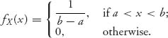
It is a model of picking a number at random from the interval [a, b] in which every number has equal likelihood. The cdf is FX(x) = (x − a)/(b − a), a ≤ x ≤ b. The mean is E[X] = {(a + b)/2, the midpoint, and variance is Var(X) = (b − a)2/12.
![]()
Then the mean is E[X] = μ, and the variance is Var(X) = σ2. The graph of fX is the classic bell-shaped curve centered at μ. The central limit theorem makes this the most important distribution because it roughly says that sums of independent random variables normalized by ![]() converge to a normal distribution, no matter what the distribution of the random variables in the sum. More precisely
converge to a normal distribution, no matter what the distribution of the random variables in the sum. More precisely
![]()
Here, E[Xi] = μ and Var(Xi) = σ2 are the mean and variance of the arbitrary members of the sum.
![]()
The density is ![]() Then E[X] = 1/λ and Var(X) = 1/λ2.
Then E[X] = 1/λ and Var(X) = 1/λ2.
B.3 Order Statistics
In the theory of auctions, one needs to put in order the valuations of each bidder and then calculate things such as the mean of the highest valuation, the second highest valuation, and so on. This is an example of the use of order statistics, which is an important topic in probability theory. We review a basic situation.
Let X1, X2, …, Xn be a collection of independent and identically distributed random variables with common density function f(x) and common cumulative distribution function F(x). The order statistics are the random variables
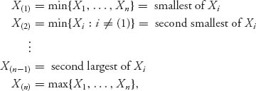
and automatically X(1) ≤ X(2) ≤ ··· ≤ X(n). This simply reorders the random variables from smallest to largest.
To get the density function of X(k), we may argue formally that X(k) ≤ x if and only if k − 1 of the random variables are ≤ x and n − k of the random variables are > x. In symbols,
![]()
This leads to the cumulative distribution function of X(k). Consequently, it is not too difficult to show that the density of X(k) is
![]()
where
![]()
because there are
![]()
ways of splitting up n things into three groups of size k − 1, n − k, and 1.
If we start with a uniform distribution f(x) = 1, 0 < x < 1, we have
![]()
If k = n − 1, then
![]()
Consequently, for X1, …, Xn independent uniform random variables, we have E(X(n−1)) = (n − 1)/(n + 1). The means and variances of all the order statistics can be found by integration.