
5.3 Duels (Optional)
Duels are used to model not only the actual dueling situation but also many problems in other fields. For example, a battle between two companies for control of a third company or asset can be regarded as a duel in which the accuracy functions could represent the probability of success. Duels can be used to model competitive auctions between two bidders. So there is ample motivation to study a theory of duels.
In earlier chapters we considered discrete versions of a duel in which the players were allowed to fire only at certain distances. In reality, a player can shoot at any distance (or time) once the duel begins. That was only one of our simplifications. The theory of duels includes multiple bullets, machine gun duels, silent and noisy, and so on.18
Here are the precise rules that we use here. There are two participants, I and II, each with a gun, and each has exactly one bullet. They will fire their guns at the opponent at a moment of their own choosing. The players each have functions representing their accuracy or probability of killing the opponent, say, pI(x) for player I and pII(y) for player II, with x, y ![]() [0, 1]. The choice of strategies is a time in [0, 1] at which to shoot. Assume that pI(0) = pII(0) = 0 and pI(1) = pII(1) = 1. So, in the setup here you may assume that they are farthest apart at time 0 or x = y = 0 and closest together when x = y = 1. It is realistic to assume also that both pI and pII are continuous, are strictly increasing, and have continuous derivatives up to any order needed.
[0, 1]. The choice of strategies is a time in [0, 1] at which to shoot. Assume that pI(0) = pII(0) = 0 and pI(1) = pII(1) = 1. So, in the setup here you may assume that they are farthest apart at time 0 or x = y = 0 and closest together when x = y = 1. It is realistic to assume also that both pI and pII are continuous, are strictly increasing, and have continuous derivatives up to any order needed.
Finally, if I hits II, player I receives + 1 and player II receives −1, and conversely. If both players miss, the payoff is 0 to both. The payoff functions will be the expected payoff depending on the accuracy functions and the choice of the x ![]() [0, 1] or y
[0, 1] or y ![]() [0, 1] at which the player will take the shot. We could take more general payoffs to make the game asymmetric as we did in Example 3.14, for instance, but we will consider only the symmetric case with continuous strategies.
[0, 1] at which the player will take the shot. We could take more general payoffs to make the game asymmetric as we did in Example 3.14, for instance, but we will consider only the symmetric case with continuous strategies.
We break our problem down into the cases where player I shoots before player II, player II shoots before player I, or they shoot at the same time.
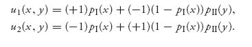
If player I shoots before player II, then x < y, and
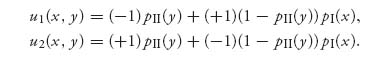
If player II shoots before player I, then y < x and we have similar expected payoffs:
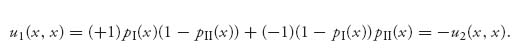
Finally, if they choose to shoot at the same time, then x = y and we have
In this simplest setup, this is a zero sum game, but, as mentioned earlier, it is easily changed to nonzero sum.
We have set up this duel without consideration yet that the duel is noisy. Each player will hear (or see, or feel) the shot by the other player, so that if a player shoots and misses, the surviving player will know that all she has to do is wait until her accuracy reaches 1. With certainty that occurs at x = y = 1, and she will then take her shot. In a silent duel, the players would not know that a shot was taken (unless they didn’t survive). Silent duels are more difficult to analyze, and we will consider a special case later.
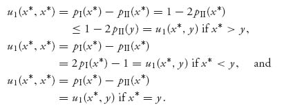
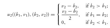
Let’s simplify the payoffs in the case of a noisy duel. In that case, when a player takes a shot and misses, the other player (if she survives) waits until time 1 to kill the opponent with certainty. So, the payoffs become
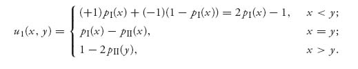
For player II, u2(x, y) = −u1(x, y).
Now, to solve this, we cannot use the procedure outlined using derivatives, because this function has no derivatives exactly at the places where the optimal things happen.
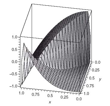
Figure 5.6 shows a graph of u1(x, y) in the case when the players have the distinct accuracy functions given by pI(x) = x3 and pII(x) = x2. Player I’s accuracy function increases at a slower rate than that for player II. Nevertheless, we will see that both players will fire at the same time. That conclusion seems reasonable when it is a noisy duel. If one player fires before the opponent, the accuracy suffers, and, if it is a miss, death is certain.
FIGURE 5.6 u1(x, y) with accuracy functions pI = x3, pII = x2.
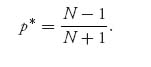
In fact, we will show that there is a unique point x* ![]() [0, 1] that is the unique solution of
[0, 1] that is the unique solution of
so that
and
This says that (x*, x*) is a Nash equilibrium for the noisy duel. Of course, since u2 = −u1, the inequalities reduce to
![]()
so that (x*, x*) is a saddle point for u1.
To verify that the inequalities (5.4) and (5.5) hold for x* defined in (5.3), we have, from the definition of u1, that
![]()
Using the fact that both accuracy functions are increasing, we have, by (5.3)
So, in all cases u1(x*, x*) ≤ u1(x*, y) for all y ![]() [0, 1]. We verify (5.5) in a similar way and leave that as an exercise. We have shown that (x*, x*) is indeed a Nash point.
[0, 1]. We verify (5.5) in a similar way and leave that as an exercise. We have shown that (x*, x*) is indeed a Nash point.
That x* exists and is unique is shown by considering the function f(x) = pI(x) + pII(x). We have f(0) = 0, f(1) = 2, and f′(x) = pI′(x) + pII′(x) > 0. By the intermediate value theorem of calculus we conclude that there is an x* satisfying f(x*) = 1. The uniqueness of x* follows from the fact that pI and pII are strictly increasing.
In the example shown in Figure 5.6 with pI(x) = x3 and pII (x) = x2, we have the condition x*3 + x*2 = 1, which has solution at x* = 0.754877. With these accuracy functions, the duelists should wait until less than 25% of the time is left until they both fire. The expected payoff to player I is u1(x*, x*) = −0.1397, and the expected payoff to player II is u2(x*, x*) = 0.1397. It appears that player I is going down. We expect that result in view of the fact that player II has greater accuracy at x*, namely, pII(x*) = 0.5698 > pI(x*) = 0.4301.
The following Maple commands are used to get all of these results and see some great pictures:
 > restart:with(plots):
 > p1: = x- > x^3;p2: = x- > x^2;
 > v1: = (x, y)- > piecewise(x < y, 2*p1(x)-1, x = y, p1(x)-p2(x), x > y,
1-2*p2(x));
 > plot3d(v1(x, y), x = 0..1, y = 0..1, axes = boxed);
 > xstar: = fsolve(p1(x) + p2(x)-1 = 0, x);
 > v1(xstar, xstar);
For a more dramatic example, suppose that pI(x) = x3, pII(x) = x. This says that player I is at a severe disadvantage. His accuracy does not improve until a lot of time has passed (and so the duelists are closer together). In this case x* = 0.68232 and they both fire at time 0.68232 and u1(0.68232, 0.68232) = −0.365. Player I would be stupid to play this game with real bullets. That is why game theory is so important.
5.3.1 SILENT DUEL ON [0, 1] (OPTIONAL)
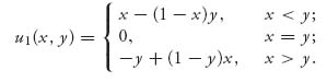
In case you are curious as to what happens when we have a silent duel, we will present this example to show that things get considerably more complicated. We take the simplest possible accuracy functions pI(x) = pII(x) = x ![]() [0, 1] because this case is already much more difficult than the noisy duel. The payoff of this game to player I is
[0, 1] because this case is already much more difficult than the noisy duel. The payoff of this game to player I is
For player II, since this is zero sum, u2(x, y) = −u1(x, y). Now, in the problem with a silent duel, intuitively it seems that there cannot be a pure Nash equilibrium because silence would dictate that an opponent could always take advantage of a pure strategy. But how do we allow mixed strategies in a game with continuous strategies? In a discrete matrix game, a mixed strategy is a probability distribution over the pure strategies. Why not allow the players to choose continuous probability distributions? No reason at all. So we consider the mixed strategy choice for each player
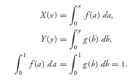
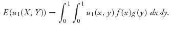
The cumulative distribution function X(x) represents the probability that player I will choose to fire at a point ≤ x. The expected payoff to player I if he chooses X and his opponent chooses Y is
As in the discrete-game case, we define the value of the game as
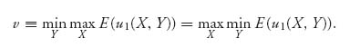
The equality follows from the existence theorem of a Nash equilibrium (actually a saddle point in this case) because the expected payoff is not only concave–convex, but actually linear in each of the probability distributions X, Y. It is completely analogous to the existence of a mixed strategy saddle point for matrix games. The value of games with a continuum of strategies exists if the players choose from within the class of probability distributions. (Actually, the probability distributions should include the possibility of point masses, but we do not go into this generality here.) A saddle point in mixed strategies has the same definition as before: (X*, Y*) is a saddle if
![]()
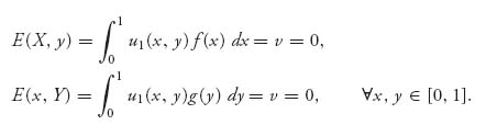
Now, the fact that both players are symmetric and have the same accuracy functions allows us to guess that v = 0 for the silent duel. To find the optimal strategies, namely, the density functions f(x), g(y), we use the necessary condition that if X*, Y* are optimal, then
This is completely analogous to the equality of payoffs Theorem 3.2.4 to find mixed strategies in bimatrix games, or to the geometric solution of two person 2 × 2 games in which the value occurs where the two payoff lines cross. We replace u1(x, y) to work with the following equation:
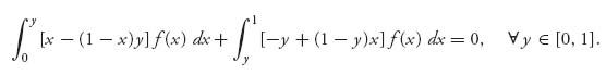
If we expand this, we get
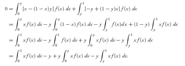
The first term in this last line is actually a constant, and the constant is E[X] = ∫01 xf(x) dx, which is the mean of the strategy X.
Now a key observation is that the equation we have should be looked at, not in the unknown function f(x), but in the unknown function xf(x). Let’s call it ![]() (x) ≡ xf(x), and we see that
(x) ≡ xf(x), and we see that
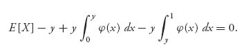
Consider the left side as a function of y ![]() [0, 1]. Call it
[0, 1]. Call it
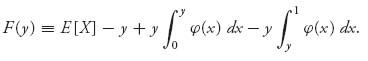
Then F(y) = 0, 0 ≤ y ≤ 1. We take a derivative using the fundamental theorem of calculus in an attempt to get rid of the integrals:
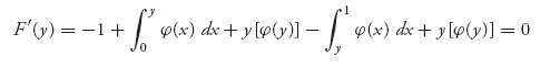
and then another derivative
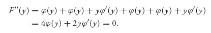
So we are led to the differential equation for ![]() (y), which is
(y), which is
![]()
This is a first-order ordinary differential equation that will have general solution
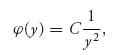
as you can easily check by plugging in. Then ![]() (y) = yf(y) =
(y) = yf(y) = ![]() implies that f(y) =
implies that f(y) = ![]() , or f(x) =
, or f(x) = ![]() returning to the x variable. We have to determine the constant C.
returning to the x variable. We have to determine the constant C.
You might think that the way to find C is to apply the fact that ∫01 f(x) dx = 1. That would normally be correct, but it also points out a problem with our formulation. Look at ∫01 x−3 dx. This integral diverges (that is, it is infinite), because x−3 is not integrable on (0, 1). This would stop us dead in our tracks because there would be no way to fix that with a constant C unless the constant was zero. That can’t be, because then f = 0, and it is not a probability density. The way to fix this is to assume that the function f(x) is zero on the starting subinterval [0, a] for some 0 < a < 1. In other words, we are assuming that the players will not shoot on the interval [0, a] for some unknown time a > 0. The lucky thing is that the procedure we used at first, but now repeated with this assumption, is the same and leads to the equation
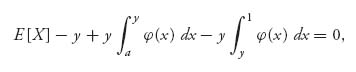
which is the same as where we were before except that 0 is replaced by a. So, we get the same function ![]() (y) and eventually the same f(x) =
(y) and eventually the same f(x) = ![]() , except we are now on the interval 0 < a ≤ x ≤ 1. This idea does not come for free, however, because now we have two constants to determine, C and a. C is easy to find because we must have ∫a1
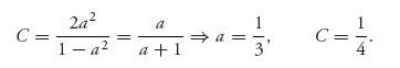
, except we are now on the interval 0 < a ≤ x ≤ 1. This idea does not come for free, however, because now we have two constants to determine, C and a. C is easy to find because we must have ∫a1 ![]() dx = 1. This says, C =
dx = 1. This says, C =  > 0. To find a > 0, we substitute f(x) =
 ![]() into (recall that
into (recall that ![]() (x) = x f(x))
(x) = x f(x))
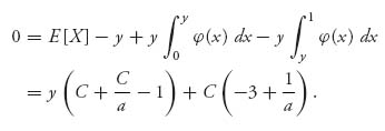
This must hold for all a ≤ y ≤ 1, which implies that C + ![]() −1 = 0. Therefore, C =
−1 = 0. Therefore, C = ![]() . But then we must have
. But then we must have
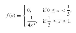
So, we have found X(x). It is the cumulative distribution function of the strategy for player I and has density
We know that ∫a1 u1(x, y)f(x)dx = 0 for y ≥ a, but we have to check that with this C = ![]() and a =
and a = ![]() to make sure that
to make sure that
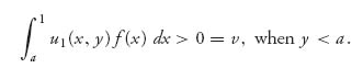
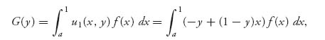
That is, we need to check that X played against any pure strategy in [0, a] must give at least the value v = 0 if X is optimal. Let’s take a derivative of the function G(y) = ∫a1 u1(x, y)f(x)dx, 0 ≤ a ≤ 1. We have,
which implies that
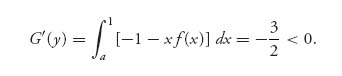
This means G(y) is decreasing on [0, a]. Since G(a) = ∫a1(−a + (1−a)x)f(x)dx = 0, it must be true that G(y) > 0 on [0, a), so the condition (5.6) checks out. Finally, since this is a symmetric game, it will be true that Y(y) will have the same density as player I.
Problem
5.42 Determine the optimal time to fire for each player in the noisy duel with accuracy functions pI(x) = sin (![]() x) and pII(x) = x2, 0 ≤ x ≤ 1.
x) and pII(x) = x2, 0 ≤ x ≤ 1.
5.4 Auctions (Optional)
There were probably auctions by cavemen for clubs, tools, skins, and so on, but we can be sure (because there is a written record) that there was bidding by Babylonians for both men and women slaves and wives. Auctions today are ubiquitous with many internet auction houses led by eBay, which does more than 6 billion dollars of business a year and earns almost 2 billion dollars as basically an auctioneer. This pales in comparison with United States treasury bills, notes, and bond auctions, which have total dollar values each year in the trillions of dollars. Rights to the airwaves, oil leases, pollution rights, and tobacco, all the way down to auctions for a Mickey Mantle-signed baseball are common occurrences.
There are different types of auctions we study. Their definitions are summarized here.
Definition 5.4.1 The different types of auctions are as follows:
- English Auction. Bids are announced publicly, and the bids rise until only one bidder is left. That bidder wins the object at the highest bid.
- Sealed Bid, First Price. Bids are private and are made simultaneously. The highest sealed bid wins and the winner pays that bid.
- Sealed Bid, Second Price. Bids are private and made simultaneously. The high bid wins, but the winner pays the second highest bid. This is also called a Vickrey auction after the Nobel Prize winner who studied them.
- Dutch Auction. The auctioneer (which could be a machine) publicly announces a high bid. Bidders may accept the bid or not. The announced prices are gradually lowered until someone accepts that price. The first bidder who accepts the announced price wins the object and pays that price.
- Private Value Auction. Bidders are certain of their own valuation of the object up for auction and these valuations (which may be random variables) are independent.
- Common Value Auction. The object for sale has the same value (that is not known for certain to the bidders) to all the bidders. Each bidder has their own estimate of this value.
In this section, we will present a game theory approach to the theory of auctions and will be more specific about the type of auction as we cover it. Common value auctions require the use of more advanced probability theory and will not be considered further.
Let’s start with a simple nonzero sum game that shows why auction firms like eBay even exist (or need to exist).
Example 5.14 In an online auction with no middleman the seller of the object and the buyer of the object may choose to renege on the deal dishonestly or go through with the deal honestly. How is that carried out? The buyer could choose to wait for the item and then not pay for it. The seller could simply receive payment but not send the item. Here is a possible payoff matrix for the buyer and the seller:
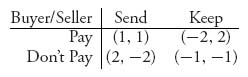
There is only one Nash equilibrium in this problem and it is at (don’t pay, keep); neither player should be honest! Amazing, the transaction will never happen and it is all due to either lack of trust on the part of the buyer and seller, or total dishonesty on both their parts. If a buyer can’t trust the seller to send the item and the seller can’t depend on the buyer to pay for the item, there won’t be a deal.
Now let’s introduce an auction house that serves two purposes: (1) it guarantees payment to the seller and (2) it guarantees delivery of the item for the buyer. Of course, the auction house will not do that out of kindness but because it is paid by the seller (or the buyer) in the form of a commission. This introduces a third strategy for the buyer and seller to use: Auctioneer. This changes the payoff matrix as follows:
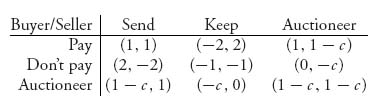
The idea is that each player has the option, but not the obligation, of using an auctioneer. If somehow they should agree to both be honest, they both get + 1. If they both use an auctioneer, the auctioneer will charge a fee of 0 < c < 1 and the payoff to each player will be 1−c.
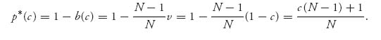
Observe that (−1, −1) is no longer a pure Nash equilibrium. We use a calculus procedure to find the mixed Nash equilibrium for this symmetric game as a function of c. The result of this calculation is
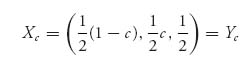
and (Xc, Yc) is the unique Nash equilibrium. The expected payoffs to each player are as follow:
![]()
As long as ![]() > c > 0, both players receive a positive expected payoff. Because we want the payoffs to be close to (1, 1), which is what they each get if they are both honest and don’t use a auctioneer, it will be in the interest of the auctioneer to make c > 0 as small as possible because at some point the transaction will not be worth the cost to the buyer or seller.
> c > 0, both players receive a positive expected payoff. Because we want the payoffs to be close to (1, 1), which is what they each get if they are both honest and don’t use a auctioneer, it will be in the interest of the auctioneer to make c > 0 as small as possible because at some point the transaction will not be worth the cost to the buyer or seller.
The Nash equilibrium tells the buyer and seller to use the auctioneer half the time, no matter what value c is. Each player should be dishonest with probability ![]() , which will increase as c increases. The players should be honest with probability only
, which will increase as c increases. The players should be honest with probability only ![]() . If c = 1 they should never play honestly and either play dishonestly or use an auctioneer half the time.
. If c = 1 they should never play honestly and either play dishonestly or use an auctioneer half the time.
You can see that the existence and only the existence of an auctioneer will permit the transaction to go through. From an economics perspective, this implies that auctioneers will come into existence as an economic necessity for online auctions and it can be a very profitable business (which it is); however, this is true not only for online auctions. Auction houses for all kinds of specialty and nonspecialty items (like horses, tobacco, diamonds, gold, houses, etc.) have been in existence for decades, if not centuries, because they serve the economic function of guaranteeing the transaction.
A common feature of auctions is that the seller of the object may set a price, called the reserve price, so that if none of the bids for the object are above the reserve price the seller will not sell the object. One question that arises is whether sellers should use a reserve price. Here is an example to illustrate.
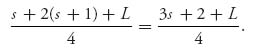
Example 5.15 Assume that the auction has two possible buyers. The seller must have some information, or estimates, about how the buyers value the object. Perhaps these are the seller’s own valuations projected onto the buyers. Suppose that the seller feels that each buyer values the object at either $s (small amount) or $L (large amount) with probability ![]() each. But, assuming bids may go up by a minimum of $1, the winning bids with no reserve price set are $s, $(s+1), $(s+1), or $L each with probability
each. But, assuming bids may go up by a minimum of $1, the winning bids with no reserve price set are $s, $(s+1), $(s+1), or $L each with probability ![]() . Without a reserve price, the expected payoff to the seller is
. Without a reserve price, the expected payoff to the seller is
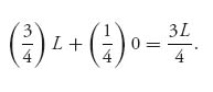
Suppose next that the seller sets a reserve price at the higher valuation $L, and this is the lowest acceptable price to the seller. Let Bi, i = 1, 2 denote the random variable that is the bid for buyer i. Without collusion or passing of information we may assume that the Bi values are independent. The seller is assuming that the valuations of the bidders are (s, s), (s, L), (L, s) and (L, L), each with probability ![]() . If the reserve price is set at $L, the sale will not go through 25% of the time, but the expected payoff to the seller will be
. If the reserve price is set at $L, the sale will not go through 25% of the time, but the expected payoff to the seller will be
The question is whether it can happen that there are valuations s and L, so that
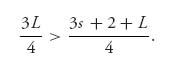
Solving for L, the requirement is that L > ![]() , and this certainly has solutions. For example, if L = 100, any lower valuation s < 66 will lead to a higher expected payoff to the seller with a reserve price set at $100. Of course, this result depends on the valuations of the seller.
, and this certainly has solutions. For example, if L = 100, any lower valuation s < 66 will lead to a higher expected payoff to the seller with a reserve price set at $100. Of course, this result depends on the valuations of the seller.
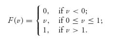
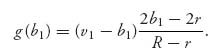
Example 5.16 If you need more justification for a reserve price, consider that if only one bidder shows up for your auction and you must sell to the high bidder, then you do not make any money at all unless you set a reserve price. Of course, the question is how to set the reserve price. Assume that a buyer has a valuation of your gizmo at $V, where V is a random variable with cumulative distribution function F(v). Then, if your reserve price is set at $p, the expected payoff (assuming one bidder) will be
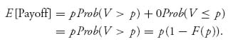
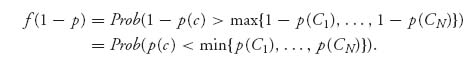
You want to choose p to maximize this function g(p) ≡ p(1−F(p)). Let’s find the critical points assuming that f(p) = F′(p) is the probability density function of V:
![]()
Assuming that g′′ (p) = 2f(p) + pf′(p) ≥ 0, we will have a maximum. Observe that the maximum is not achieved at p = 0 because g′(0) = 1−F(0) = 1 > 0. So, we need to find the solution, p*, of
![]()
For a concrete example, we assume that the random variable V has a normal distribution with mean 0.5 and standard deviation 0.2. The density is
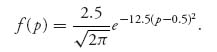
We need to solve 1−F(p)−pf(p) = 0, where F(p) is the cumulative normal distribution with mean 0.5 and standard deviation 0.2. This is easy to do using Maple. The Maple commands to get our result are as follows:
> restart:
> with(Statistics):
> X := RandomVariable(Normal(0.5, 0.2)):
> plot(1-CDF(X, u)-u*PDF(X, u), u=0..1);
> fsolve(1-CDF(X, u)-u*PDF(X, u), u);
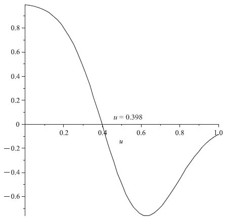
The built-in functions PDF and CDF give the density and cumulative normal functions. We have also included a command to give us a plot of the function giving the root. The plot of b(u) = 1−F(u)−u f(u) is shown in Figure 5.7.
We see that the function b(u) crosses the axis at u = p* =0.398. The reserve price should be set at 39.8% of the maximum valuation.
Having seen why auction houses exist, let’s get into the theory from the bidders’ perspective. There are N bidders (=players) in this game. There is one item up for bid and each player values the object at v1 ≥ v2 ≥ · · · ≥ v_N > 0 dollars. One question we have to deal with is whether the bidders know this ranking of values.
FIGURE 5.7 Graph of 1−F(u)−u f(u) with V Normal (0.5, 0.22).
5.4.1 COMPLETE INFORMATION
In the simplest and almost totally unrealistic model, all the bidders have complete information about the valuations of all the bidders. Now we define the rules of the auctions considered in this section.
Definition 5.4.2 A first-price, sealed-bid auction is an auction in which each bidder submits a bid bi, i = 1, 2, …, N in a sealed envelope. After all the bids are received the envelopes are opened by the auctioneer and the person with the highest bid wins the object and pays the bid bi. If there are identical bids, the winner is chosen at random from the identical bidders.
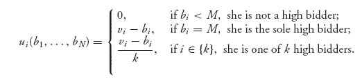
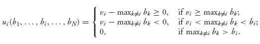
What is the payoff to player i if the bids are b1, …, bN? Well, if bidder i doesn’t win the object, she pays nothing and gets nothing. That will occur if she is not a high bidder:
![]()
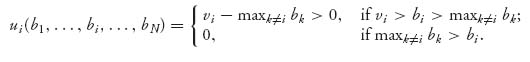
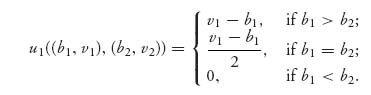
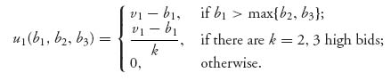
On the other hand, if she is a high bidder, so that bi = M, then the payoff is the difference between what she bid and what she thinks it’s worth (i.e., vi−bi). If she bids less than her valuation of the object, and wins the object, then she gets a positive payoff, but she gets a negative payoff if she bids more than it’s worth to her. To take into account the case when there are k ties in the high bids, she would get the average payoff. Let’s use the notation that { k } is the set of high bidders. So, in symbols
Naturally, bidder i wants to know the amount to bid. That is determined by finding the maximum payoff of player i, assuming that the other players are fixed. We want a Nash equilibrium for this game. This doesn’t really seem too complicated. Why not just bid vi? That would guarantee a payoff of zero to each player, but is that the maximum? Should a player ever bid more than her valuation? These questions are answered in the following rules.
With complete information and a sealed-bid first-price auction bidders should bid as follows:
Problems
5.43 Verify that in the first-price auction (b1, …, bN) = (v1, …, vN) is a Nash equilibrium assuming v1 = v2.
5.44 In a second-price sealed-bid auction with complete information the winner is the high bidder but she pays, not the price she bid, but the second highest bid. If there are ties, then the winner is drawn at random from among the high bidders and she pays the highest bid. Formulate the payoff functions and show that the following rules are optimal:
5.45 A homeowner is selling her house by auction. Two bidders place the same value on the house at $100, 000, while the next bidder values the house at $80, 000. Should the homeowner use a first-price or second-price auction to sell the house, or does it matter? What if the highest valuation is $100, 000, the next is $95, 000 and the rest are no more than $90, 000?
5.46 Find the optimal reserve price to set in an auction assuming that the density of the value random variable V is f(p) = 6p(1−p), 0 ≤ p ≤ 1.
5.4.2 INCOMPLETE INFORMATION
The setup now is that we have N > 1 bidders with valuations of the object for sale Vi, i = 1, 2, …, N. The problem is that the valuations are not known to either the buyers or the seller, except for their own valuation. Thus, since we must have some place to start we assume that the seller and buyers think of the valuations as random variables. The information that we assume known to the seller is the joint cumulative distribution function
![]()
and each buyer i has knowledge of his or her own distribution function Fi(vi) = P(Vi ≤ vi).
5.4.2.1 Take-It-or-Leave-It Rule This is the simplest possible problem that may still be considered an auction. But it is not really a game. It is a problem of the seller of an object as to how to set the buy-it-now price.
In an auction, you may set a reserve price r, which, as we have seen, is a nonnegotiable lowest price you must get to consider selling the object. You may also declare a price p ≥ r, which is your take-it-or-leave-it price or buy-it-now price and wait for some buyer, who hopefully has a valuation greater than or equal to p to buy the object. The problem is to determine p.
The solution involves calculating the expected payoff from the trade and then maximizing the expected payoff over p ≥ r. The payoff is the function U(p), which is p−r, if there is a buyer with a valuation at least p, and 0 otherwise:
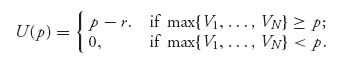
This is a random variable because it depends on V1, …, VN, which are random. The expected payoff is
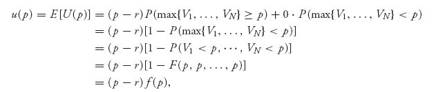
where f(p) = 1−F(p, p, …, p). The seller wants to find p* such that
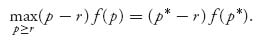
If there is a maximum p* > r, we could find it by calculus. It is the solution of
![]()
This will be a maximum as long as (p* −r)f′′(p*) + 2f′(p*) ≤ 0. To proceed further, we need to know something about the valuation distribution. Let’s take the simplest case that { Vi} is a collection of N independent and identically distributed random variables. In this case
![]()
Then
![]()
is the density function of Vi, if it is a continuous random variable. So the condition for a maximum at p* becomes
![]()
Now we take a particular distribution for the valuations that is still realistic. In the absence of any other information, we might as well assume that the valuations are uniformly distributed over the interval [r, R], remembering that r is the reserve price. For this uniform distribution, we have
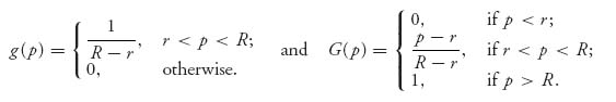
If we assume that r < p* < R, then we may solve
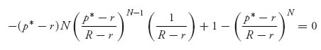
for p* to get the take-it-or-leave-it price
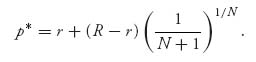
For this p*, we have the expected payoff
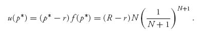
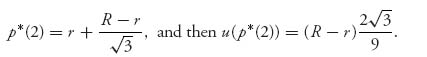
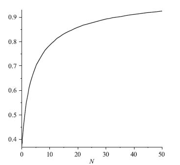
Of particular interest are the cases N = 1, N = 2, and N → ∞. We label the take-it-or-leave-it price as p* = p* (N). Here are the results:
![]()
the midpoint of the range [r, R]. The expected payoff to the seller is
![]()
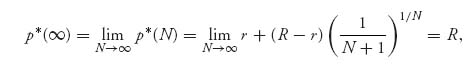
and then the expected payoff is u(p* (∞)) = R−r. Note that we may calculate limN → ∞ (1/N + 1)1/N = 1 using L’Hôpital’s rule. We conclude that as the number of potential buyers increases, the price should be set at the upper range of valuations. A totally reasonable result.
You can see from Figure 5.8, which plots p* (N) as a function of N (with R = 1, r = 0), that as the number of buyers increases, there is a rapid increase in the take-it-or-leave-it price before it starts to level off.
FIGURE 5.8 Take-it-or-leave-it price versus number of bidders.
5.4.3 SYMMETRIC INDEPENDENT PRIVATE VALUE AUCTIONS
In this section19 we take it a step further and model the auction as a game. Again, there is one object up for auction by a seller and the bidders know their own valuations of the object but not the valuations of the other bidders. It is assumed that the unknown valuations V1, …, VN are independent and identically distributed continuous random variables. The symmetric part of the title of this section comes from assuming that the bidders all have the same valuation distribution.
We will consider two types of auction:
Remarks A Dutch auction is equivalent to the first-price sealed-bid auction. Why? A bidder in each type of auction has to decide how much to bid to place in the sealed envelope or when to yell “Buy” in the Dutch auction. That means that the strategies and payoffs are the same for these types of auction. In both cases, the bidder must decide the highest price she is willing to pay and submit that bid. In a Dutch auction, the object will be awarded to the highest bidder at a price equal to her bid. That is exactly what happens in a first-price sealed-bid auction. The strategies for making a bid are identical in each of the two seemingly different types of auction.
An English auction can also be shown to be equivalent to a second-price sealed-bid auction (as long as we are in the private values set up). Why? As long as bidders do not change their valuations based on the other bidders’ bids, which is assumed, then bidders should accept to pay any price up to their own valuations. A player will continue to bid until the current announced price is greater than how much the bidder is willing to pay. This means that the item will be won by the bidder who has the highest valuation and she will win the object at a price equal to the second highest valuation.
The equivalence of the various types of auctions was first observed by William Vickrey.20 The result of an English auction can be achieved by using a sealed-bid auction in which the item is won by the second highest submitted bid. A bidder should submit a bid that is equal to her valuation of the object since she is willing to pay an amount less than her valuation but not willing to pay a price greater than her valuation. Assuming that each player does that, the result of the auction is that the object will be won by the bidder with the highest valuation and the price paid will be the second highest valuation.
For simplicity, it will be assumed that the reserve price is normalized to r = 0. As above, we assume that the joint distribution function of the valuations is given by
![]()
which holds because we assume independence and identical distribution of the bidder’s valuations. Suppose that the maximum possible valuation of all the players is a fixed constant w > 0. Then, a bidder gets to choose a bidding function bi(v) that takes points in [0, w] and gives a positive real bid. Because of the symmetry property, it should be the case that all players have the same payoff function and that all optimal strategies for each player are the same for all other players.
Now suppose that we have a player with bidding function b = b(v) for a valuation v ![]() [0, w]. The payoff to the player is given by
[0, w]. The payoff to the player is given by
![]()
We have to use the expected payment for the bid b(v) because we don’t know whether the bid b(v) will be a winning bid. The probability that b(v) is the high bid is
![]()
We will simplify notation a bit by setting
![]()
and then write the payoff as
![]()
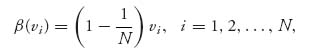
We want the bidder to maximize this payoff by choosing a bidding strategy β (v).
One property of β (v) should be obvious, namely, as the valuation increases, the bid must increase. The fact that β (v) is strictly increasing as a function of v can be proved using some convex analysis but we will skip the proof.
Once we know the strict increasing property, the fact that all bidders are essentially the same leads us to the conclusion that the bidder with the highest valuation wins the auction.
Let’s take the specific example that bidder’s valuations are uniform on [0, w] = [0, 1]. Then for each player, we have
Remark Whenever we say in the following that we are normalizing to the interval [0, 1], this is not a restriction because we may always transform from an interval [r, R] to [0, 1] and the reverse by the linear transformation t = (s−r)/(R−r), r ≤ s ≤ R, or s = r + (R−r)t, 0 ≤ t ≤ 1.
We can now establish the following theorem.21
Theorem 5.4.3 Suppose that valuations V1, …, VN, are uniformly distributed on [0, 1], and the expected payoff function for each bidder is
Then there is a unique Nash equilibrium (β, …, β) given by
![]()
in the case when we have an English auction, and
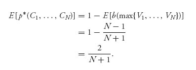
in the case when we have a Dutch auction. In either case the expected payment price for the object is
Proof To see why this is true, we start with the Dutch auction result. Since all players are indistinguishable, we might as well say our that guy is player 1. Suppose that player 1 bids b = β (v). Then the probability that she wins the object is given by
![]()
Now here is where we use the fact that β is strictly increasing, because then it has an inverse, v = β−1(b), and so we can say
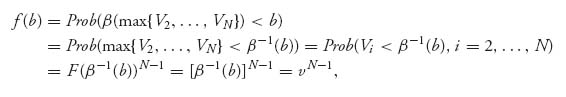
because all valuations are independent and identically distributed. The next-to-last-equality is because we are assuming a uniform distribution here. The function f(b) is the probability of winning the object with a bid of b. ![]()
Now, for the given bid b = β (v), player 1 wants to maximize her expected payoff. The expected payoff (5.7) becomes
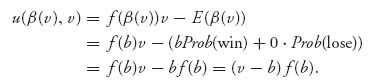
Taking a derivative of u(b, v) with respect to b, evaluating at b = β (v) and setting to zero, we get the condition
Since f(b) = [β−1(b)]N−1 = vN−1, v = β−1(b), we have
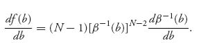
Therefore, after dividing out the term [β−1(b)]N−2, the condition (5.8) becomes
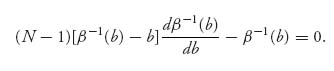
Let’s set y(b) = β−1(b) to see that this equation becomes
This is a first-order ordinary differential equation for y(b), that we may solve to get
Actually, we may find the general solution of (5.9) using Maple fairly easily. The Maple commands to do this are as follows:
 > ode: = a*(y(x)-x)*diff(y(x), x) = y(x);
 > dsolve(ode, y(x));
That’s it, just two commands without any packages to load. We are setting a = N−1. Here is what Maple gives you:
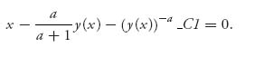
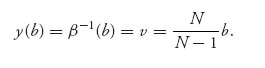
The problem with this is that we are looking for the solution with y(0) = 0 because when the valuation of the item is zero, the bid must be zero. Note that the term y(x)−a is undefined if y(0) = 0. Consequently, we must take C1 = 0, leaving us with x−(a/(a + 1))y(x) = 0 that gives y(x) = ((a + 1)/a)x. Now we go back to our original variables to get y(b) = v = β−1(b) = (N/(N−1))b. Solving for b in terms of v, we get
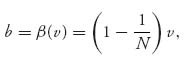
which is the claimed optimal bidding function in a Dutch auction.
Next, we calculate the expected payment. In a Dutch auction, we know that the payment will be the highest bid. We know that is going to be the random variable β (max { V1, …, VN}), which is the optimal bidding function evaluated at the largest of the random valuations. Then
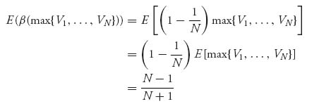
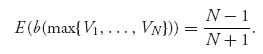
because E[max { V1, …, VN}] = ![]() , as we will see next, when the Vi values are uniform on [0, 1].
, as we will see next, when the Vi values are uniform on [0, 1].
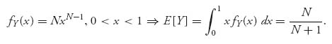
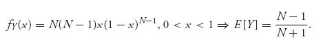
Here is why E[max { V1, …, VN} ] = N/(N + 1). The cumulative distribution function of Y = max { V1, …, VN} is derived as follows. Since the valuations are independent and all have the same distribution,
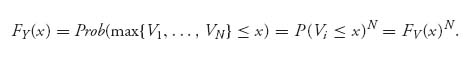
Then the density of Y is
![]()
In case V has a uniform distribution on [0, 1], fV(x) = 1, FV(x) = x, 0 < x < 1, and so
So we have verified everything for the Dutch auction case.
Next, we solve the English auction game. We have already discussed informally that in an English auction each bidder should bid his or her true valuation so that β (v) = v. Here is a formal statement and proof.
Theorem 5.4.4 In an English auction with valuations V1, …, VN and Vi = vi known to player i, then player i’s optimal bid is vi.
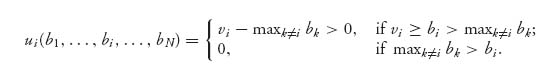
Proof 1. Suppose that player i bids bi > vi, more than her valuation. Recall that an English auction is equivalent to a second-price sealed-bid auction. Using that we calculate her payoff as
(We are ignoring possible ties.) To see why this is her payoff, if vi ≥ maxk ≠ ibk, then player i’s valuation is more than the bids of all the other players, so she wins the auction (since bi > vi) and pays the highest bid of the other players (which is maxk ≠ ibk), giving her a payoff of vi −maxk ≠ ibk > 0.
If vi > maxk ≠ i bk < bi, she values the object as less than at least one other player but bids more than this other player. So she pays maxk ≠ ibk, and her payoff is vi − maxk ≠ ibk > 0. In the last case, she does not win the object, and her payoff is zero.
2. If player i’s bid is bi ≤ vi, then her payoff is
So, in all cases the payoff function in (5.11) is at least as good as the payoff in (5.10) and better in some cases. Therefore, player i should bid bi ≤ vi.
3. Now what happens if player i bids bi < vi? In that case,
Player i will get a strictly positive payoff if vi > bi > maxk ≠ ibk.
Putting steps (3) and (2) together, we therefore want to maximize the payoff for player i using bids bi subject to the constraint vi ≥ bi > maxk ≠ ibk. Looking at the payoffs, the biggest that ui can get is when bi = vi. In other words, since bi < vi and the probability increases:
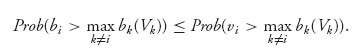
The largest probability, and therefore the largest payoff, will occur when bi = vi. ![]()
Having proved that the optimal bid in an English auction is bi = β (vi) = vi, we next calculate the expected payment and complete the proof of Theorem 28. The winner of the English auction with uniform valuations makes the payment of the second highest bid, which is given by
![]()
This follows from knowing the density of the random variable Y = maxi ≠ j{ Vi}, the second highest valuation. In the case when V is uniform on [0, 1] the density of Y is
You can refer to the Appendix B for a derivation of this using order statistics. Therefore we have proved all parts of Theorem 28.
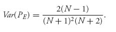
One major difference between English and Dutch auctions is the risk characteristics as measured by the variance of the selling price (see Wolfstetter (1996) for the derivation):
![]()
Consequently,
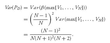
We claim that Var(PD) > Var(PE). That will be true if
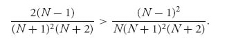
After using some algebra, this inequality reduces to the condition 2 > ![]() , which is absolutely true for any N ≥ 1. We conclude that Dutch auctions are less risky for the seller than are English auctions, as measured by the variance of the payment.
, which is absolutely true for any N ≥ 1. We conclude that Dutch auctions are less risky for the seller than are English auctions, as measured by the variance of the payment.
If the valuations are not uniformly distributed, the problem will be much harder to solve explicitly. But there is a general formula for the Nash equilibrium still assuming independence and that each valuation has distribution function F(v). If the distribution is continuous, the Dutch auction will have a unique Nash equilibrium given by
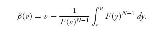
The proof of this formula comes basically from having to solve the differential equation that we derived earlier for the Nash equilibrium:
![]()
where we have set y(b) = β−1(b), and F(y) is the cumulative distribution function and f = F′ is the density function.
The expected payment in a Dutch auction with uniformly distributed valuations was shown to be E[PD] = ![]() . The expected payment in an English auction was also shown to be E[PE] =
. The expected payment in an English auction was also shown to be E[PE] = ![]() . You will see in the problems that the expected payment in an all-pay auction, in which all bidders will have to pay their bid, is also
. You will see in the problems that the expected payment in an all-pay auction, in which all bidders will have to pay their bid, is also ![]() . What’s going on? Is the expected payment for an auction always
. What’s going on? Is the expected payment for an auction always ![]() , at least for valuations that are uniformly distributed? The answer is “Yes, ” and not just for uniform distributions:
, at least for valuations that are uniformly distributed? The answer is “Yes, ” and not just for uniform distributions:
Theorem 5.4.5 Any symmetric private value auction with identically distributed valuations, satisfying the following conditions, always has the same expected payment to the seller of the object:
This is known as the revenue equivalence theorem.
In the remainder of this section, we will verify directly as sort of a review that linear trading rules are the way to bid when the valuations are uniformly distributed in the interval [r, R], where r is the reserve price. For simplicity, we consider only two bidders who will have payoff functions:
and
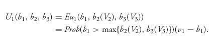
We have explicitly indicated that each player has two variables to work with, namely, the bid and the valuation. Of course, the bid will depend on the valuation eventually. The independent valuations of each player are random variables V1, V2 with identical cumulative distribution function FV(v). Each bidder knows his or her own valuation but not the opponent’s. So the expected payoff to player 1 is
![]()
because in all other cases the expected value is zero. In the case b1 = b2(V2) it is zero since we have continuous random variables. In addition, we write player 1’s bid and valuation with lower case letters because player 1 knows her own bid and valuation with certainty. Similarly,
![]()
A Nash equilibrium must satisfy
![]()
In the case that the valuations are uniform on [r, R], we will verify that the bidding rules
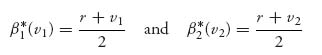
constitute a Nash equilibrium. We only need to show it is true for β1* because it will be the same procedure for β2*.
So, by the assumptions, we have
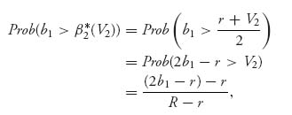
if ![]() < b
< b![]() , and the expected payoff
, and the expected payoff
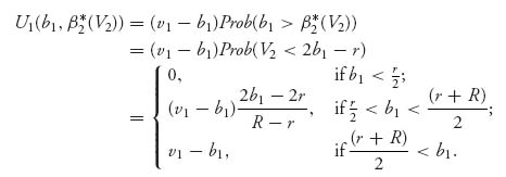
We want to maximize this as a function of b1. To do so, let’s consider the case ![]() < b1 <
< b1 < ![]() and set
and set
The function g is strictly concave down as a function of b1 and has a unique maximum at β1 = ![]() +
+ ![]() , as the reader can readily verify by calculus. We conclude that β1* (v1) =
, as the reader can readily verify by calculus. We conclude that β1* (v1) = ![]() maximizes U1(b1, β2*). This shows that β1* (v1) is a best response to β2* (v2). We have verified the claim.
maximizes U1(b1, β2*). This shows that β1* (v1) is a best response to β2* (v2). We have verified the claim.
Remark A similar argument will work if there are more than two bidders. Here are the details for three bidders. Start with the payoff functions (we give only the one for player 1 since the others are similar):
The expected payoff if player 1 knows her own bid and valuation, but V2, V3 are random variables is
Assuming independence of valuations, we obtain
![]()
In the exercises you will find the optimal bidding functions.
Example 5.17 Two players are bidding in a first-price sealed-bid auction for a 1901s US penny, a very valuable coin for collectors. Each player values it at somewhere between $750K (where K = 1000) and $1000K dollars with a uniform distribution (so r = 750, R = 1000). In this case, each player should bid βi(vi) = ![]() (750 + vi). So, if player 1 values the penny at $800K, she should optimally bid β1(800) = 775K. Of course, if bidder 2 has a higher valuation, say, at $850K, then player 2 will bid β2(850) =
(750 + vi). So, if player 1 values the penny at $800K, she should optimally bid β1(800) = 775K. Of course, if bidder 2 has a higher valuation, say, at $850K, then player 2 will bid β2(850) = ![]() (750 + 850) = 800K and win the penny. It will sell for $800K and player 2 will benefit by 850-800 = 50K.
(750 + 850) = 800K and win the penny. It will sell for $800K and player 2 will benefit by 850-800 = 50K.
On the other hand, if this were a second-price sealed-bid auction, equivalent to an English auction, then each bidder would bid their own valuations. In this case, b1 = $800K and b2 = $850K. Bidder 2 still gets the penny, but the selling price is the same. On the other hand, if player 1 valued the penny at $775K, then b1 = $775K, and that would be the selling price. It would sell for $25K less than in a first-price auction.
We conclude with a very nice application of auction theory to economic models appearing in the survey article by Wolfstetter (1996).
Example 5.18 Application of Auctions to Bertrand’s Model of Economic Competition. If we look at the payoff for a bidder in a Dutch auction we have seen in Theorem 28
![]()
where
![]()
Compare u with the profit function in a Bertrand model of economic competition. This looks an awful lot like a profit function in an economic model by identifying v as price per gadget, b as a cost, and f(b) as the probability the firm sets the highest price. That is almost correct but not exactly. Here is the exact analogy.
We consider Bertrand’s model of competition between N ≥ 2 identical firms. Assume that each firm has a constant and identical unit cost of production c > 0, and that each firm knows its own cost but not those of the other firms. For simplicity, we assume that each firm considers the costs of the other firms as random variables with a uniform distribution on [0, 1].
A basic assumption in the Bertrand model of competition is that the firm offering the lowest price at which the gadgets are sold will win the market. With that assumption, we may make the Bertrand model to be a Dutch auction with a little twist, namely, the buyers are bidding to win the market at the lowest selling price of the gadgets. So, if we think of the market as the object up for auction, each firm wants to bid for the object and obtain it at the lowest possible selling price, namely, the lowest possible price for the gadgets.
We take a strategy to be a function that converts a unit cost for the gadget (valuation) into a price for the gadget. Then we equate the price to set for a gadget to a bid for the object (market).
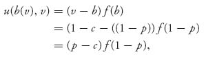
The Bertrand model is really an inverse Dutch auction, so if we invert variables, we should be able to apply the Dutch auction results. Here is how to do that. Call a valuation v = 1−c. Then call the price to be set for a gadget as one minus the bid, p = 1−b, or b = 1−p. In this way, low costs lead to high valuations, and low prices imply higher bids, and conversely. So the highest bid (= lowest price) wins the market. The expected payoff function in the Dutch auction is then
where
Putting them together, we have
![]()
as the profit function to each firm, because w(p, c) is the expected net revenue to the firm if the firm sets price p for a gadget and has cost of production c per gadget, but the firm has to set the lowest price for a gadget to capture the market.
Now in a Dutch auction we know that the optimal bidding function is b(v) = ((N − 1)/N)v, so that
This is the optimal expected price to set for gadgets as a function of the production cost. Next, the expected payment in a Dutch auction is
So
We conclude that the equilibrium expected price of gadgets in this model for each firm as a function of the unit cost of production will be
Problem
5.47 In an all-pay auction, all the bidders must actually pay their bids to the seller, but only the high bidder gets the object up for sale. This type of auction is also called a charity auction. By following the procedure for a Dutch auction, show that the equilibrium bidding function for all players is β (v) = ((N−1)/N) vN, assuming that bidders’ valuations are uniformly distributed on the normalized interval [0, 1]. Find the expected total amount collected by the seller.
Bibliographic Notes
The voter model in Example 5.3 is a standard application of game theory to voting. More than two candidates are allowed for a model to get an N > 2 person game. Here, we follow the presentation in the reference by Aliprantis and Chakrabarti (2000) in the formulation of the payoff functions.
The economics models presented in Section 5.2 have been studied for many years, and these models appear in both the game theory and economic theory literature. The generalization of the Cournot model in Theorem 5.2.1 due to Wald is proved in full generality in the book by Parthasarathy and Raghavan (1991). The Bertrand model and its ramifications follows Ferguson (2013) and Aliprantis and Chakrabarti (2000). The traveler’s paradox Example 5.9 (from Goeree and Holt (1996)) is also well known as a critique of both the Nash equilibrium concept and a Bertrand-type model of markets. Entry deterrence is a modification of the same model in Ferguson’s notes (2013). The theory of duels as examples of games of timing is due to Karlin (1992). Our derivation of the payoff functions and the solution of the silent continuous duel also follows Karlin (1992).
The land division game in Problem 5.22 is a wonderful calculus and game theory problem. For this particular geometry of land we take the formulation in Jones (2000). Problem 5.17 is formulated as an advertising problem in Ferguson (2013). Gintis (2000) is an outstanding source of problems in many areas of game theory. Problems 5.23 and 5.21 are modifications of the tobacco farmer problem and Social Security problem in Gintis (2000).
The theory of auctions has received considerable interest since the original analysis by W. Vickrey beginning in the 1960s. In this section, we follow the survey by Wolfstetter (1996), where many more results are included. In particular, we have not discussed the theory of auctions with a common value because it uses conditional expectations, which is beyond our level of prerequisites. The application of auction theory to solving an otherwise complex Bertrand economic model in Example 5.18 is presented by Wolfstetter (1996). The direct verification that linear trading rules form a Nash equilibrium is from Aliprantis and Chakrabarti (2000).
1 The arg max of a function is the set of points where the maximum is attained.
2 This example is adapted from a similar example in Aliprantis and Chakrabarti (2000), commonly known as the median voter problem.
3 Due to Professor Dietrich Braess, Mathematics Department, Ruhr University Bochum, Germany.
4 Adapted from an example in Goeree and Holt (1999).
5 This is an advanced topic and may be skipped without loss of continuity.
6 More generally one would have to take a mixed strategy as a cumulative distribution function F1(x) = Prob(I plays q ≤ x) and F1′(x) = X(x). But not every cdf has a pdf.
7 f is upper semicontinuous if { x|f(x) < a} is open for each a ![]()
![]() .
.
8 The solution of this game is due to James Webb (2006).
9 Robert Aumann (born June 8, 1930) won a Nobel Memorial Prize in Economic Sciences, 2005.
10 John Harsanyi (born May 29, 1920 in Budapest, Hungary; died August 9, 2000 in Berkeley, California, United States) won a Nobel Memorial Prize in Economic Sciences 1994.
11 Roger Myerson (born March 29, 1951) won a Nobel Memorial Prize in Economic Sciences, 2007.
12 Thomas Schelling (born April 14, 1921) won a Nobel Memorial Prize in Economic Sciences, 2005.
13 Reinhard Selten (born October 5, 1930) won the 1994 Nobel Memorial Prize in Economic Sciences (shared with John Harsanyi and John Nash).
14 Antoine Augustin Cournot (August 28, 1801–March 31, 1877) was a French philosopher and mathematician. One of his students was Auguste Walras, who was the father of Leon Walras. Cournot and Auguste Walras convinced Leon Walras to give economics a try. Walras then came up with his famous equilibrium theory in economics.
15 October 31, 1902–December 13, 1950. Wald was a mathematician born in Hungary who made fundamental contributions to statistics, probability, differential geometry, and econometrics. He was a professor at Columbia University at the time of his death in a plane crash in India.
16 Joseph Louis François Bertrand, March 11, 1822 − April 5, 1900, a French mathematician who contributed to number theory, differential geometry, probability theory, thermodynamics, and economics. He reviewed the Cournot competition model, arguing that Cournot had reached a misleading conclusion.
17 Heinrich Freiherr von Stackelberg (1905 − 1946) was a German economist who contributed to game theory and oligopoly theory.
18 Refer to Karlin’s (1992) book for a very nice exposition of the general theory of duels.
19 Refer to the article by Milgrom (1989) for an excellent essay on auctions from an economic perspective.
20 William Vickrey 1914–1996 won the 1996 Nobel Prize in economics primarily for his foundational work on auctions. He earned a BS in mathematics from Yale in 1935 and a PhD in economics from Columbia University.
21 See the article by Wolfstetter (1996) for a very nice presentation and many more results on auctions, including common value auctions.