
Problems
6.25 There are three types of planes (1, 2, and 3) that use an airport runway. Plane 1 needs a 100-yard runway, 2 needs a 150-yard runway, and 3 needs a 400-yard runway. The cost of maintaining a runway is equal to its length. Suppose this airport has one 400-yard runway used by all three types of planes and assume also that only one plane of each type will land at the airport on a given day. We want to know how much of the $400 cost should be allocated to each plane.
6.26 In a glove game with three players, player 1 can supply one left glove and players 2 and 3 can supply one right glove each. The value of a coalition is the number of paired gloves in the coalition.
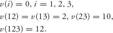
6.27 Consider the normalized characteristic function for a three-person game:
![]()
Find the core, the least core X1, and the next least core X2. X2 will be the nucleolus.
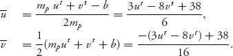
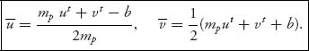
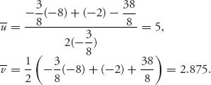
6.28 Find the fair allocation in the nucleolus for the three-person characteristic function game with
6.29 In Problem 6.12, we considered the problem in which companies can often get a better cash return if they invest larger amounts. There are three companies who may cooperate to invest money in a venture that pays a rate of return as follows:
| Invested amount | Rate of return |
| 0–1, 000, 000 | 4% |
| 1, 000, 000–3, 000, 000 | 5% |
| >3, 000, 000 | 5.5% |
Suppose company 1 will invest $1, 800, 000, company 2, $900, 000, and company 3, $400, 000. This problem was considered earlier but with a different amount of cash for player 3. How should the net amount earned on the total investment be split among the three companies? Define an appropriate characteristic function. Find the nucleolus.
6.30 There are three ambitious computer science students, named 1, 2, and 3, with a lucrative idea and they wish to start a business. None of the students can start a business on their own, but any two of them can:
- If 1 and 2 form a business, their total salary will be 120, 000.
- If 1 and 3 form a business, their total salary will be 100, 000.
- If 2 and 3 form a business, their total salary will be 80, 000.
- If all three go into business together, they will pay themselves a total salary of 150, 000.
6.31 Four doctors, Moe, Larry, Curly, and Shemp, 4 are in partnership and cover hours for each other. At most one doctor needs to be in the office to see patients at any one time. They advertise their office hours as follows:
| (1) | Shemp | 12:00–5:00 |
| (2) | Curly | 9:00–4:00 |
| (3) | Larry | 10:00–4:00 |
| (4) | Moe | 2:00–5:00 |
A coalition is an agreement by one or more doctors as to the times they will really be in the office to see everybody’s patients. The characteristic function should be the amount of time saved by a given coalition. Note that v(i) = 0, and v(1234) = 13 hours. This problem is an example of the use of cooperative game theory in an scheduling problem and is an important application in many disciplines.
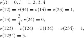
6.32 Use software to solve the four-person game with unnormalized characteristic function
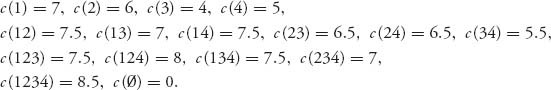
6.33 We have four players involved in a game to minimize their costs. We have transformed such games to savings games by defining v(S) = ∑i ![]() S c(i) − c(S), the total cost if each player is in a one-player coalition, minus the cost involved if players form the coalition S. Find the nucleolus allocation of costs for the four-player game with costs
S c(i) − c(S), the total cost if each player is in a one-player coalition, minus the cost involved if players form the coalition S. Find the nucleolus allocation of costs for the four-player game with costs
6.34 Show that in a cost savings game if we define the cost savings characteristic function v(S) = ∑i ![]() S c(i) − c(S), if v(S) is superadditive, then c(S) is subadditive, and conversely.
S c(i) − c(S), if v(S) is superadditive, then c(S) is subadditive, and conversely.
6.3 The Shapley Value
In an entirely different approach to deciding a fair allocation in a cooperative game, we change the definition of fair from minimizing the maximum dissatisfaction to allocating an amount proportional to the benefit each coalition derives from having a specific player as a member. The fair allocation would be the one recognizing the amount that each member adds to a coalition. Players who add nothing should receive nothing, and players who are indispensable should be allocated a lot. The question is how do we figure out how much benefit each player adds to a coalition. Lloyd Shapley5 came up with a way.
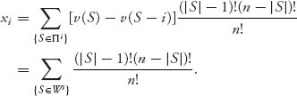
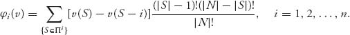
Definition 6.3.1 An allocation ![]() = (x1, …, xn) is called the Shapley value if
= (x1, …, xn) is called the Shapley value if
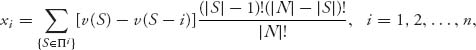
where Πi is the set of all coalitions S ![]() N containing i as a member (i.e., i
N containing i as a member (i.e., i ![]() S), |S| = number of members in S, and |N| = n.
S), |S| = number of members in S, and |N| = n.
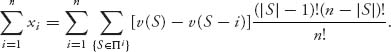
If players join the grand coalition one after the other we know that there are n! possible sequences. Assume the probability of any particular sequence forming is then ![]() . When player i shows up and finds S − i players already there, then i′s contribution is to the coalition S is v(S) − v(S − i). The Shapley allocation is each player’s expected contribution to any possible sequencing of players joining the grand coalition.
. When player i shows up and finds S − i players already there, then i′s contribution is to the coalition S is v(S) − v(S − i). The Shapley allocation is each player’s expected contribution to any possible sequencing of players joining the grand coalition.
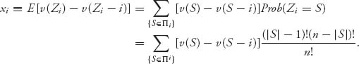
More precisely, fix a player, say, i, and consider the random variable Zi, which takes its values in the set of all possible coalitions 2N. Zi is the coalition S in which i is the last player to join S and n − |S| players join the grand coalition after player i. Diagrammatically, if i joins the coalition S on the way to the formation of the grand coalition, we have
![]()
Remember that because a characteristic function is superadditive, the players have the incentive to form the grand coalition.
For a given coalition S, by elementary probability, there are (|S| − 1)!(n − |S|)! ways i can join the grand coalition N, joining S first. With this reasoning, we assume that Zi has the probability distribution.
![]()
We choose this distribution because |S| − 1 players have joined before player i, and this can happen in (|S| − 1)! ways; and n − |S| players join after player i, and this can happen in (n − |S|)! ways. The denominator is the total number of ways that the grand coalition can form among n players. Any of the n! permutations has probability ![]() of actually being the way the players join. This distribution assumes that they are all equally likely. One could debate this choice of distribution, but this one certainly seems reasonable. Also, see Example 6.17 below for a direct example of the calculation of the arrival of a player to a coalition and the consequent benefits.
of actually being the way the players join. This distribution assumes that they are all equally likely. One could debate this choice of distribution, but this one certainly seems reasonable. Also, see Example 6.17 below for a direct example of the calculation of the arrival of a player to a coalition and the consequent benefits.
Therefore, for the fixed player i, the benefit player i brings to the coalition Zi is v(Zi) − v(Zi − i). It seems reasonable that the amount of the total grand coalition benefits that should be allocated to player i should be the expected value of v(Zi) − v(Zi − i). This gives
The Shapley value (or vector) is then the allocation ![]() = (x1, …, xn). At the end of this chapter, you can find the Maple code to find the Shapley value.
= (x1, …, xn). At the end of this chapter, you can find the Maple code to find the Shapley value.
Example 6.14 Two players have to divide $M, but they each get zero if they can’t reach an agreement as to how to divide it. What is the fair division? Obviously, without regard to the benefit derived from the money the allocation should be M/2 to each player. Let’s see if Shapley gives that.
Define v(1) = v(2) = 0, v(12) = M. Then
![]()
Note that if we solve this problem using the least core approach, we get
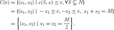
The reason for this is that if x1 ≥ −ε, x2 ≥ −ε, then adding, we have −2ε ≤ x1 + x2 = M. This implies that ε ≥ −M/2, is the restriction on ε. The first ε that makes C(ε) ≠ ![]() is then ε1 = −M/2. Then x1 ≥ M/2, x2 ≥ M/2 and, since they add to M, it must be that x1 = x2 = M/2. So the least core allocation and the Shapley value coincide in the problem.
is then ε1 = −M/2. Then x1 ≥ M/2, x2 ≥ M/2 and, since they add to M, it must be that x1 = x2 = M/2. So the least core allocation and the Shapley value coincide in the problem.
Before we continue, let’s verify that in fact the Shapley allocation actually satisfies the required conditions to be an allocation, namely individual and group rationality.
First, we show that xi ≥ v(i), i = 1, 2, …, n, that is, individual rationality is satisfied. To see this, since v(S) ≥ v(S − i) + v(i) by superadditivity, we have
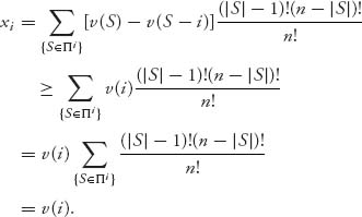
The last equality follows from the fact that
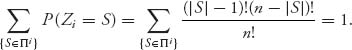
Second, we have to show the Shapley allocation satisfies group rationality, that is, ∑i = 1n xi = v(N). Let’s add up the xi′s,
By carefully analyzing the coefficients in the double sum we can show that group rationality holds. Instead of going through that let’s just look at the case n = 2. We have
Example 6.15 Let’s go back to the sink allocation (Example 6.8) with Amy, Agnes, and Agatha. Using the core concept, we obtained
| Player | Truck capacity | Allocation |
| Amy | 45 | 35 |
| Agnes | 60 | 50 |
| Agatha | 75 | 65 |
| Total | 180 | 150 |
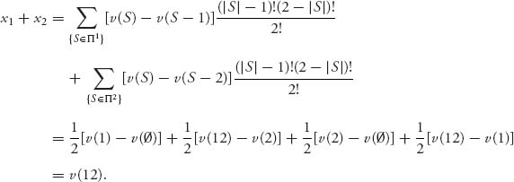
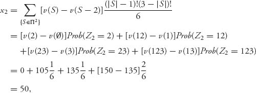
Let’s see what we get for the Shapley value. Recall that the characteristic function was v(i) = 0, v(13) = 120, v(12) = 105, v(23) = 135, v(123) = 150. In this case, n = 3, n! = 6 and for player i = 1, Π1 = {1, 12, 13, 123}, so
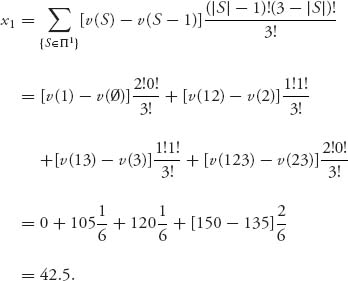
Similarly, with Π2 = {2, 12, 23, 123},
and with Π3 = {3, 13, 23, 123}
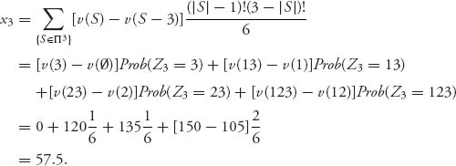
Consequently, the Shapley vector is ![]() = (42.5, 50, 57.5), or, since we can’t split sinks
= (42.5, 50, 57.5), or, since we can’t split sinks ![]() = (43, 50, 57), an allocation quite different from the nucleolus solution of (35, 50, 65).
= (43, 50, 57), an allocation quite different from the nucleolus solution of (35, 50, 65).
Example 6.16 A typical and interesting fair allocation problem involves a debtor who owes money to more than one creditor. The problem is that the debtor does not have enough money to pay off the entire amount owed to all the creditors. Consequently, the debtor must negotiate with the creditors to reach an agreement about what portion of the assets of the debtor will be paid to each creditor. Usually, but not always, these agreements are imposed by a bankruptcy court.
Let’s take a specific problem. Suppose that debtor D has exactly $100, 000 to pay off three creditors A, B, C. Debtor D owes A $50, 000; D owes B $65, 000, and D owes C $10, 000.
Now it is possible for D to split up the $100K (K=1000) on the basis of percentages; that is, the total owed is $125, 000 and the amount owed to A is 40% of that, to B is 52%, and to C about 8%, so A would get $40K, B would get $52K and C would get $8K. What if the players could form coalitions to try to get more?
Let’s take the characteristic function as follows. The three players are A, B, C and (with amounts in thousands of dollars)
![]()
To explain this choice of characteristic function, consider the coalition consisting of just A. If we look at the worst that could happen to A, it would be that B and C get paid off completely and A gets what’s left, if anything. If B gets $65K and C gets $10K then $25K is left for A, and so we take v(A) = 25. Similarly, if A and B get the entire $100K, then C gets $0. If we consider the coalition AC they look at the fact that in the worst case B gets paid $65K and they have $35K left as the value of their coalition. This characteristic function is a little pessimistic since it is also possible to consider that AC would be paid $75K and then v(AC) = 75. So other characteristic functions are certainly possible. On the other hand, if two creditors can form a coalition to freeze out the third creditor not in the coalition, then the characteristic function we use here is exactly the result.
Now we compute the Shapley values. For player A, we have

Similarly, for players B and C
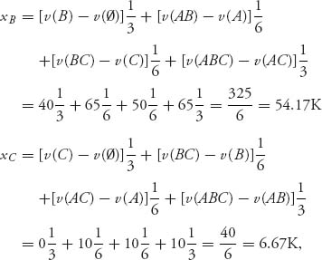
where again K = 1000. The Shapley allocation is ![]() = (39.17, 54.17, 6.67) compared to the allocation by percentages of (40, 52, 8). Player B will receive more under the Shapley allocation at the expense of players A and C, who are owed the least.
= (39.17, 54.17, 6.67) compared to the allocation by percentages of (40, 52, 8). Player B will receive more under the Shapley allocation at the expense of players A and C, who are owed the least.
A reasonable question to ask is why is the Shapley allocation any better than the percentage allocation? After all, the percentage allocation gives a perfectly reasonable answer—or does it? Actually, if players can combine to freeze out another player (especially in a court of law with lawyers involved), or if somehow coalitions among the creditors can form, then the percentage allocation ignores the power of the coalition. The players do not all have the same negotiating power. The Shapley allocation takes that into account through the characteristic function, while the percentage allocation does not.
Example 6.17 A typical problem facing small biotech companies is that they can discover a new drug, but they don’t have the resources to manufacture and market it. Typically the solution is to team up with a large partner. Let’s say that A is the biotech firm and B and C are the candidate big pharmaceutical companies. If B or C teams up with A, the big firm will split $1 billion with A. Here is a possible characteristic function:
![]()
We will indicate a quicker way to calculate the Shapley allocation when there are a small number of players. We make a table indicating the value brought to a coalition by each player on the way to formation of the grand coalition:
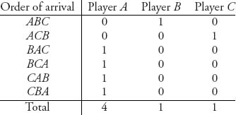
The numbers in the table are the amount of value added to a coalition when that player arrives. For example, if A arrives first, no benefit is added; then, if B arrives and joins A, player B has added 1 to the coalition AB; finally, when C arrives (so we have the coalition ABC), C adds no additional value. Since it is assumed in the derivation of the Shapley value that each arrival sequence is equally likely we calculate the average benefit brought by each player as the total benefit brought by each player (the sum of each column), divided by the total number of possible orders of arrival. We get
![]()
So company A, the discoverer of the drug should be allocated two-thirds of the $1 billion and the big companies split the remaining third.
It is interesting to compare this with the nucleolus. The core, which will be the nucleolus for this example, is
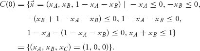
This says that A gets the entire $1 billion and the other companies get nothing. The Shapley value is definitely more realistic.
Shapley vectors can also quickly analyze the winning coalitions in games where winning or losing is all we care about: who do we team up with to win. Here are the definitions.
Definition 6.3.2 Suppose that we are given a characteristic function v(S) that satisfies that for every S ![]() N, either v(S) = 0 or v(S) = 1. This is called a simple game. If v(S) = 1, the coalition S is said to be a winning coalition. If v(S) = 0, the coalition S is said to be a losing coalition. Let
N, either v(S) = 0 or v(S) = 1. This is called a simple game. If v(S) = 1, the coalition S is said to be a winning coalition. If v(S) = 0, the coalition S is said to be a losing coalition. Let
![]()
denote the set of coalitions who win with player i and lose without player i. These are the winning coalitions for which player i is critical.
Simple games are very important in voting systems. For example, a game in which the coalition with a majority of members wins has v(S) = 1, if |S| > n/2, as the winning coalitions. Losing coalitions have |S| ≤ n/2 and v(S) = 0. If only unanimous votes win, then v(N) = 1 is the only winning coalition. Finally, if there is a certain player who has dictatorial power, say, player 1, then v(S) = 1 if 1 ![]() S and v(S) = 0 if 1
S and v(S) = 0 if 1 ![]() S.
S.
In the case of a simple game for player i we need only consider coalitions S ![]() Πi for which S is a winning coalition, but S − i, that is, S without i, is a losing coalition. We have denoted that set by Wi. We need only consider S
Πi for which S is a winning coalition, but S − i, that is, S without i, is a losing coalition. We have denoted that set by Wi. We need only consider S ![]() Wi because v(S) − v(S − i) = 1 only when v(S) = 1, and v(S − i) = 0. In all other cases v(S) − v(S − i) = 0. In particular, it is an exercise to show that v(S) = 0 implies that v(S − i) = 0 and v(S − i) = 1 implies that v(S) = 1. Hence, the Shapley value for a simple game is
Wi because v(S) − v(S − i) = 1 only when v(S) = 1, and v(S − i) = 0. In all other cases v(S) − v(S − i) = 0. In particular, it is an exercise to show that v(S) = 0 implies that v(S − i) = 0 and v(S − i) = 1 implies that v(S) = 1. Hence, the Shapley value for a simple game is
The Shapley allocation for player i represents the power that player i holds in a game. You can think of it as the probability that a player can tip the balance. It is also called the Shapley–Shubik index and is very important in political science.
Example 6.18 A corporation has four stockholders (with 100 total shares) who all vote their own individual shares on any major decision. The majority of shares voted decides an issue. A majority consists of more than 50 shares. Suppose that the holdings of each stockholder are as follows:
![]()
The winning coalitions, that is, with v(S) = 1 are as follows:
![]()
We find the Shapley allocation. For x1, it follows that W1 = {123} because S = {123} is winning but S − 1 = {23} is losing. Hence,
![]()
Similarly, W2 = {24, 123, 124}, and so
![]()
Also, x3 = ![]() and x4 =
and x4 = ![]() . We conclude that the Shapley allocation for this game is
. We conclude that the Shapley allocation for this game is ![]() = (
= (![]() ,
, ![]() ,
, ![]() ,
, ![]() ). Note that player 1 has the least power, but players 2 and 3 have the same power even though player 3 controls 10 more shares than does player 2. Player 4 has the most power, but a coalition is still necessary to constitute a majority.
). Note that player 1 has the least power, but players 2 and 3 have the same power even though player 3 controls 10 more shares than does player 2. Player 4 has the most power, but a coalition is still necessary to constitute a majority.
Continue this example, but change the shares as follows:
![]()
Computing the Shapley value as x1 = 0, x2 = x3 = x4 = ![]() , we see that player 1 is completely marginalized as she contributes nothing to any coalition. She has no power. In addition, player 4’s additional shares over players 2 and 3 provide no advantage over those players since a coalition is essential to carry a majority in any case.
, we see that player 1 is completely marginalized as she contributes nothing to any coalition. She has no power. In addition, player 4’s additional shares over players 2 and 3 provide no advantage over those players since a coalition is essential to carry a majority in any case.
Example 6.19 The United Nations Security Council has 15 members, 5 of whom are permanent (Russia, Great Britain, France, China, and the United States). These five players have veto power over any resolution. To pass a resolution requires all five permanent member’s votes and four of the remaining 10 nonpermanent member’s votes. This is a game with fifteen players, and we want to determine the Shapley–Shubik index of their power. We label players 1, 2, 3, 4, 5 as the permanent members.
Instead of the natural definition of a winning coalition as one that can pass a resolution, it is easier to use the definition that a winning coalition is one that can defeat a resolution. So, for player 1 the winning coalitions are those for which S ![]() Π1, and v(S) = 1, v(S − 1) = 0; that is, player 1, or player 1 and any number up to six nonpermanent members can defeat a resolution, so that the winning coalitions for player 1 is the set
Π1, and v(S) = 1, v(S − 1) = 0; that is, player 1, or player 1 and any number up to six nonpermanent members can defeat a resolution, so that the winning coalitions for player 1 is the set
![]()
where the letters denote distinct nonpermanent members. The number of distinct two-player winning coalitions that have player 1 as a member is ![]() , 6 three-player coalitions is
, 6 three-player coalitions is ![]() , four-player coalitions is
, four-player coalitions is ![]() , and so on, and each of these coalitions will have the same coefficients in the Shapley value. So we get
, and so on, and each of these coalitions will have the same coefficients in the Shapley value. So we get
![]()
We can use Maple to give us the result with this command:
> tot:=0;
> for k from 0 to 6 do
    tot:=tot+binomial(10, k)*k!*(14-k)!/15!
    end do:
> print(tot);
We get x1 = ![]() = 0.1963. Obviously, it must also be true that x2 = x3 = x4 = x5 = 0.19623. The five permanent members have a total power of 5 × 0.19623 = 0.9812 or 98.12% of the power, while the nonpermanent members have x6 = · · · = x15 = 0.0019 or 0.19% each, or a total power of 1.88%.
= 0.1963. Obviously, it must also be true that x2 = x3 = x4 = x5 = 0.19623. The five permanent members have a total power of 5 × 0.19623 = 0.9812 or 98.12% of the power, while the nonpermanent members have x6 = · · · = x15 = 0.0019 or 0.19% each, or a total power of 1.88%.
Example 6.20 In this example, 7 we show how cooperative game theory can determine a fair allocation of taxes to a community. For simplicity, assume that there are only four households and that the community requires expenditures of $100, 000. The question is how to allocate the cost of the $100, 000 among the four households.
As in most communities, we consider the wealth of the households as represented by the value of their property. Suppose the wealth of household i is wi. Our four households have specific wealth values
![]()
again with units in thousands of dollars. In addition, suppose that there is a cap on the amount that each household will have to pay (on the basis of age, income, or some other factors) that is independent of the value of their property value. In our case, we take the maximum amount each of the four households will be required to pay as
![]()
What is the fair allocation of expenses to each household?
Let’s consider the general problem first. Define the variables:
| T | Total costs of community |
| ui | Maximum amount i will have to pay |
| wi | Net worth of player i |
| zi | Amount player i will have to pay |
| ui − zi | Surplus of the cap over the assessment |
The quantity ui − zi is the difference between the maximum amount that household i would ever have to pay and the amount household i actually pays. It represents the amount household i does not have to pay.
We will assume that the total wealth of all the players is greater than T, and that the total amount that the players are willing (or are required) to pay is greater than T, but the total actual amount that the players will have to pay is exactly T:
This makes sense because “you can’t squeeze blood out of a turnip.” Here is the characteristic function we will use:
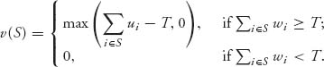
In other words, v(S) = 0 in two cases: (1) if the total wealth of the members of coalition S is less than the total cost, ∑i ![]() S wi < T, or (2) if the total maximum amount coalition S is required to pay is less than T, ∑i
S wi < T, or (2) if the total maximum amount coalition S is required to pay is less than T, ∑i ![]() S ui < T. If a coalition S cannot afford the expenditure T, then the characteristic function of that coalition is zero.
S ui < T. If a coalition S cannot afford the expenditure T, then the characteristic function of that coalition is zero.
The Shapley value involves the expression v(S) − v(S − j) in each term. Only the terms with v(S) − v(S − j) > 0 need to be considered.
Suppose first that the coalition S and player j ![]() S satisfies v(S) > 0 and v(S − j) > 0. That means the coalition S and the coalition S without player j can finance the community. We compute
S satisfies v(S) > 0 and v(S − j) > 0. That means the coalition S and the coalition S without player j can finance the community. We compute
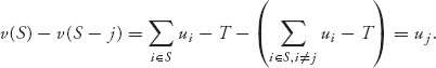
Next, suppose that the coalition S can finance the community, but not without j: v(S) > 0, v(S − j) = 0. Then
![]()
Summarizing the cases, we have
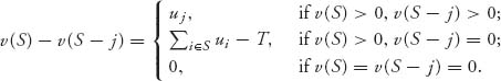
Note that if j ![]() S and v(S − j) > 0, then automatically v(S) > 0. We are ready to compute the Shapley allocation. For player j = 1, …, n, we have
S and v(S − j) > 0, then automatically v(S) > 0. We are ready to compute the Shapley allocation. For player j = 1, …, n, we have
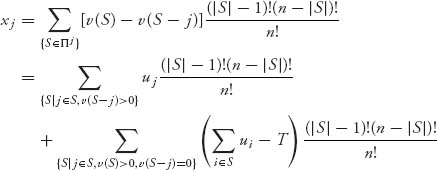
By our definition of the characteristic function for this problem, the allocation xj is the portion of the surplus ∑i ui − T > 0 that will be assessed to household j. Consequently, the amount player j will be billed is actually zj = uj − xj.
For the four-person problem data above we have T = 100, ∑ wi = 750 > 100, ∑i ui = 155 > 100, so all our assumptions in (6.5) are verified. Remember that the units are in thousands of dollars. Then we have
![]()
For example, v(134) = max(u1 + u3 + u4 − 100, 0) = 125 − 100 = 25. We compute
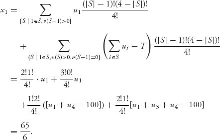
The first term comes from coalition S = 124; the second term comes from coalition S = 1234; the third term comes from coalition S = 14; and the last term from coalition S = 134.
As a result, the amount player 1 will be billed will be z1 = u1 − x1 = 25 − ![]() =
= ![]() thousand dollars. In a similar way, we calculate
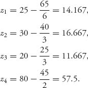
thousand dollars. In a similar way, we calculate
![]()
so that the actual bill to each player will be
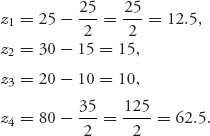
For comparison purposes, it is not too difficult to calculate the nucleolus for this game to be ![]()
![]() , 15, 10,
, 15, 10, ![]()
![]() , so that the payments using the nucleolus will be
, so that the payments using the nucleolus will be
There is yet a third solution, the straightforward solution that assesses the amount to each player in proportion to each household’s maximum payment to the total assessment. For example, u1/(∑i ui) = 25/155 = 0.1613 and so player 1 could be assessed the amount 0.1613 × 100 = 16.13.
We end this section by explaining how Shapley actually came up with his fair allocation, because it is very interesting in its own right.
First, we separate players who don’t really matter. A player i is a dummy if for any coalition S in which i ![]() S, we have
S, we have
![]()
So dummy player i contributes nothing to any coalition. The players who are not dummies are called the carriers of the game. Let’s define C = set of carriers.
Shapley now looked at things this way. Given a characteristic function v, we should get an allocation as a function of v, ![]() (v) = (
(v) = (![]() 1 (v), …,
1 (v), …, ![]() n (v)), where
n (v)), where ![]() i(v) will be the allocation or worth or value of player i in the game, and this function
i(v) will be the allocation or worth or value of player i in the game, and this function ![]() should satisfy the following properties:
should satisfy the following properties:
The last property is the strongest and most controversial. It essentially says that the allocation to a player using the sum of characteristic functions should be the sum of the allocations corresponding to each characteristic function.
Now these properties, if you agree that they are reasonable, lead to a surprising conclusion. There is one and only one function ![]() that satisfies them! It is given by
that satisfies them! It is given by ![]() (v) = (
(v) = (![]() 1(v), …,
1(v), …, ![]() n(v)), where
n(v)), where
This is the only function satisfying the properties, and, sure enough, it is the Shapley value.
Problems
6.35 The formula for the Shapley value is
![]()
where Πi is the set of all coalitions S ![]() N containing i as a member (i.e., i
N containing i as a member (i.e., i ![]() S). Show that an equivalent formula is
S). Show that an equivalent formula is
![]()
6.36 Let v be a superadditive characteristic function for a simple game. Show that if v(S) = 0 and A ![]() S then v(A) = 0 and if v(S) = 1 and S
S then v(A) = 0 and if v(S) = 1 and S ![]() A then v(A) = 1.
A then v(A) = 1.
6.37 Moe, Larry, and Curly have banded together to form a leg, back, and lip waxing business, LBLWax, Inc. The overhead to the business is 40K per year. Each stooge brings in annual business and incurs annual costs as follows: Moe-155K revenue, 40K costs; Larry-160K revenue, 35K costs; Curly-140K revenue, 38K costs. Costs include, wax, flame throwers, antibiotics, and so on. Overhead includes rent, secretaries, insurance, and so on. At the end of each year, they take out all the profit and allocate it to the partners.
6.38 In Problems 6.12 and 6.29, we considered the problem in which three investors can earn a greater rate of return if they invest together and pool their money. Find the Shapley values in both cases discussed in those exercises.
6.39 Three chiropractors, Moe, Larry, and Curly, are in partnership and cover hours for each other. At most one chiropractor needs to be in the office to see patients at any one time. They advertise their office hours as follows:
| (1) | Moe | 2:00–5:00 |
| (2) | Larry | 11:00–4:00 |
| (3) | Curly | 9:00–1:00 |
A coalition is an agreement by one or more doctors as to the times they will really be in the office to see everyone’s patients. The characteristic function should be the amount of time saved by a given coalition.
Find the Shapley value using the table of order of arrival.
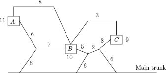
6.40 In the figure, three locations are connected as in the network. The numbers on the branches represent the cost to move one unit along that branch. The goal is to connect each location to the main trunk and to each other in the most economical way possible. The benefit of being connected to the main trunk is shown next to each location. Branches can be traversed in both directions. Take the minimal cost path to the main trunk in all cases.
6.41 Suppose that the seller of an object (which is worthless to the seller) has two potential buyers who are willing to pay $100 or $130, respectively.
6.42 Consider the characteristic function in Example 6.16 for the creditor–debtor problem. By writing out the table of the order of arrival of each player versus the benefit the player brings to a coalition when the player arrives as in Example 6.17, calculate the Shapley value.
6.43 Find the Shapley allocation for the three-person characteristic function game with
6.44 Once again we consider the four doctors, Moe (4), Larry (3), Curly (2), and Shemp (1), and their problem to minimize the amount of hours they work as in Problem 6.31. The characteristic function is the number of hours saved by a coalition. We have v(i) = 0 and
![]()
Find the Shapley allocation.
6.45 Garbage Game. Suppose that there are four property owners each with one bag of garbage that needs to be dumped on somebody’s property (one of the four). Find the Shapley value for the garbage game with v(N) = −4 and v(S) = −(4 − |S|).
6.46 A farmer (player 1) owns some land that he values at $100K. A speculator (player 2) feels that if she buys the land, she can subdivide it into lots and sell the lots for a total of $150K. A home developer (player 3) thinks that he can develop the land and build homes that he can sell. So the land to the developer is worth $160K.
6.47 Find the Shapley allocation for the cost game in Problem 6.33.
6.48 Consider the five-player game with v(S) = 1 if 1 ![]() S and |S| ≥ 2, v(S) = 1 if |S| ≥ 4 and v(S) = 0 otherwise. Player 1 is called Mr BIG, and the others are called Peons. Find the Shapley value of this game. (Hint: Use symmetry to simplify.)
S and |S| ≥ 2, v(S) = 1 if |S| ≥ 4 and v(S) = 0 otherwise. Player 1 is called Mr BIG, and the others are called Peons. Find the Shapley value of this game. (Hint: Use symmetry to simplify.)
6.49 Consider the glove game in which there are four players; player 1 can supply one left glove and players 2, 3, and 4 can supply one right glove each.
6.50 In Problem 6.25 we considered that there are three types of planes (1, 2, and 3) that use an airport. Plane 1 needs a 100-yard runway, 2 needs a 150-yard runway, and 3 needs a 400-yard runway. The cost of maintaining a runway is equal to its length. Suppose this airport has one 400-yard runway used by all three types of planes and assume that for the day under study, only one plane of each type lands at the airport. We want to know how much of the $400 cost should be allocated to each plane. We showed that the nucleolus is C(ε = −50) = {x1 = x2 = −50, x3 = −300} .
6.51 A river has n pollution-producing factories dumping water into the river. Assume that the factory does not have to pay for the water it uses, but it may need to expend money to clean the water before it can use it. Assume the cost of a factory to clean polluted water before it can be used is proportional to the number of polluting factories. Let c = cost per factory. Assume also that a factory may choose to clean the water it dumps into the river at a cost of b per factory. We take the inequalities 0 < c < b < nc. The characteristic function is
![]()
Take n = 5, b = 3, c = 2. Find the Shapley allocation.
6.52 Suppose we have a game with characteristic function v that satisfies the property v(S) + v(N − S) = v(N) for all coalitions S ![]() N. These are called constant sum games.
N. These are called constant sum games.
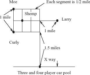
6.53 Three plumbers, Moe Howard (1), Larry Fine (2), and Curly Howard (3), work at the same company and at the same times. Their houses are located as in the figure and they would like to carpool to save money.8 Once they reach the expressway, the distance to the company is 12 miles. They drive identical Chevy Corvettes so each has the identical cost of driving to work of 1 dollar per mile. Assume that for any coalition, the route taken is always the shortest distance to pick up the passengers (doubling back may be necessary to pick someone up). It doesn’t matter whose car is used. Only the direction from home to work is to be considered. Shemp is not to be considered in this part of the problem.
6.54 An alternative to the Shapley–Shubik index is called the Banzhaf–Coleman index, which is the imputation ![]() = (b1, b2, …, bn) defined by
= (b1, b2, …, bn) defined by
![]()
where Wi is the set of coalitions that win with player i and lose without player i. We also refer to Wi as the coalitions for which player i is critical for passing a resolution. It is primarily used in weighted voting systems in which player i has wi votes, and a resolution passes if ∑j wj ≥ q, where q is known as the quota.
6.55 Suppose a game has four players with votes 4, 2, 1, 1, respectively, for each player i = 1, 2, 3, 4. The quota is q = 5. Show that the Banzhaf–Coleman index for player 1 is more than twice the index for player 2 even though player 2 has exactly half the votes player 1 does.
6.56 The Senate of the 112th Congress has 100 members of whom 53 are Democrats and 47 are Republicans. Assume that there are three types of Democrats and three types of Republicans–Liberals, Moderates, Conservatives. Assume that these types vote as a block. For the Democrats, Liberals (1) have 20 votes, Moderates (2) have 25 votes, Conservatives (3) have 8 votes. Also, for Republicans, Liberals (4) have 2 votes, Moderates (5) have 15 votes, and Conservatives (6) have 30 votes. A resolution requires 60 votes to pass.
6.4 Bargaining
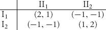
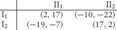
In this section, we will introduce a new type of cooperative game in which the players bargain to improve both of their payoffs. Let us start with a simple example to illustrate the benefits of bargaining and cooperation. Consider the symmetric two-player nonzero sum game with bimatrix:
You can easily check that there are three Nash equilibria given by X1 = (0, 1) = Y1, X2 = (1, 0) = Y2, and X3 = (![]() ,
, ![]() ), Y3 = (
), Y3 = (![]() ,
, ![]() ). Now consider Figure 6.9.
). Now consider Figure 6.9.
FIGURE 6.9 Payoff I versus payoff II for the prisoner’s dilemma.
The points represent the possible pairs of payoffs to each player (E1(x, y), E2(x, y)) given by
![]()
It was generated with the following Maple commands:
> with(plots):with(plottools):with(LinearAlgebra):
> A:=Matrix([[2, -1], [-1, 1]]);B:=Matrix([[1, -1], [-1, 2]]);
> f:=(x, y)->expand(Transpose(<x, 1-x>).A.<y, 1-y>);
> g:=(x, y)->expand(Transpose(<x, 1-x>).B.<y, 1-y>);
> points:={seq(seq([f(x, y), g(x, y)], x=0..1, 0.05), y=0..1, 0.05)}:
> pure:=([[2, 1], [-1, -1], [-1, -1], [1, 2]]);
> pp:=pointplot(points);
> pq:=polygon(pure, color=yellow);
> display(pq, pp, title=”Payoffs with and without cooperation”);
The horizontal axis (abscissa) is the payoff to player I, and the vertical axis (ordinate) is the payoff to player II. Any point in the parabolic region is achievable for some 0 ≤ x ≤ 1, 0 ≤ y ≤ 1.
The parabola is given by the implicit equation 5(E1 − E2)2 − 2(E1 + E2) + 1 = 0. If the players play pure strategies, the payoff to each player will be at one of the vertices. The pure Nash equilibria yield the payoff pairs (E1 = 1, E2 = 2) and (E1 = 2, E2 = 1). The mixed Nash point gives the payoff pair (E1 = ![]() , E2 =
, E2 = ![]() ), which is strictly inside the region of points, called the noncooperative payoff set.
), which is strictly inside the region of points, called the noncooperative payoff set.
Now, if the players do not cooperate, they will achieve one of two possibilities: (1) The vertices of the figure, if they play pure strategies; or (2) any point in the region of points bounded by the two lines and the parabola, if they play mixed strategies. The portion of the triangle outside the parabolic region is not achievable simply by the players using mixed strategies. However, if the players agree to cooperate, then any point on the boundary of the triangle, the entire shaded region, 9 including the boundary of the region, are achievable payoffs, which we will see shortly. Cooperation here means an agreement as to which combination of strategies each player will use and the proportion of time that the strategies will be used.
Player I wants a payoff as large as possible and thus as far to the right on the triangle as possible. Player II wants to go as high on the triangle as possible. So player I wants to get the payoff at (2, 1), and player II wants the payoff at (1, 2), but this is possible if and only if the opposing player agrees to play the correct strategy. In addition, it seems that nobody wants to play the mixed Nash equilibrium because they can both do better, but they have to cooperate to achieve a higher payoff.
Here is another example illustrating the achievable payoffs.
Example 6.21
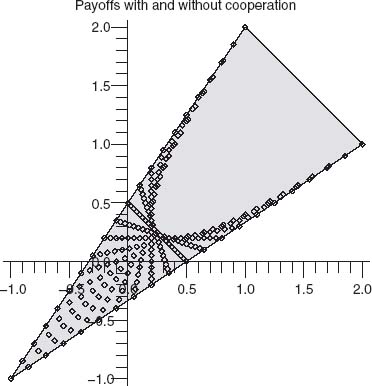
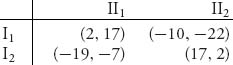
We will draw the pure payoff points of the game as the vertices of the graph and connect the pure payoffs with straight lines, as in Figure 6.10.
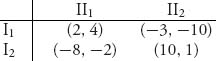
The vertices of the polygon are the payoffs from the matrix. The solid lines connect the pure payoffs. The dotted lines extend the region of payoffs to those payoffs that could be achieved if both players cooperate. For example, suppose that player I always chooses row 2, I2, and player II plays the mixed strategy Y = (y1, y2, y3), where yi ≥ 0, y1 + y2 + y3 = 1. The expected payoff to I is then
![]()
and the expected payoff to II is
![]()
Hence,
![]()
which, as a linear combination of the three points (0, −2), (3, 1), and (![]() ,
, ![]() ), is in the convex hull of these three points. This means that if players I and II can agree that player I will always play row 2, then player II can choose a (y1, y2, y3) so that the payoff pair to each player will be in the triangle bounded by the lower dotted line in Figure 6.10 and the lines connecting (0, −2) with (
), is in the convex hull of these three points. This means that if players I and II can agree that player I will always play row 2, then player II can choose a (y1, y2, y3) so that the payoff pair to each player will be in the triangle bounded by the lower dotted line in Figure 6.10 and the lines connecting (0, −2) with (![]() ,
, ![]() ) with (3, 1). The conclusion is that any point in the convex hull of all the payoff points is achievable if the players agree to cooperate.
) with (3, 1). The conclusion is that any point in the convex hull of all the payoff points is achievable if the players agree to cooperate.
One thing to be mindful of is that the Figure 6.10 does not show the actual payoff pairs that are achievable in the noncooperative game as we did for the 2 × 2 symmetric game (Figure 6.9) because it is too involved. The boundaries of that region may not be straight lines or parabolas.
The entire four-sided region in Figure 6.10 is called the feasible set for the problem. The precise definition in general is as follows.
Definition 6.4.1 The feasible set is the convex hull of all the payoff points corresponding to pure strategies of the players.
FIGURE 6.10 Achievable payoffs with cooperation.
The objective of player I in Example 6.21 is to obtain a payoff as far to the right as possible in Figure 6.10, and the objective of player II is to obtain a payoff as far up as possible in Figure 6.10. Player I’s ideal payoff is at the point (3, 1), but that is attainable only if II agrees to play II2. Why would he do that? Similarly, II would do best at (1, 4), which will happen only if I plays I1, and why would she do that? There is an incentive for the players to reach a compromise agreement in which they would agree to play in such a way so as to obtain a payoff along the line connecting (1, 4) and (3, 1). That portion of the boundary is known as the Pareto-optimal boundary because it is the edge of the set and has the property that if either player tries to do better (say, player I tries to move further right), then the other player will do worse (player II must move down to remain feasible). That is the definition. We have already defined what it means to be Pareto-optimal, but it is repeated here for convenience.
Definition 6.4.2 The Pareto-optimal boundary of the feasible set is the set of payoff points in which no player can improve his payoff without at least one other player decreasing her payoff.
The point of this discussion is that there is an incentive for the players to cooperate and try to reach an agreement that will benefit both players. The result will always be a payoff pair occuring on the Pareto-optimal boundary of the feasible set.
In any bargaining problem, there is always the possibility that negotiations will fail. Hence, each player must know what the payoff would be if there were no bargaining. This leads us to the next definition.
Definition 6.4.3 The status quo payoff point, or safety point, or security point in a two-person game is the pair of payoffs (u*, v*) that each player can achieve if there is no cooperation between the players.
The safety point usually is, but does not have to be, the same as the safety levels defined earlier. Recall that the safety levels we used in previous sections were defined by the pair (value(A), value(BT)). In the context of bargaining, it is simply a noncooperative payoff to each player if no cooperation takes place. For most problems considered in this section, the status quo point will be taken to be the values of the zero sum games associated with each player, because those values can be guaranteed to be achievable, no matter what the other player does.
Example 6.22 We will determine the security point for each player in Example 6.21. In this example, we take the security point to be the values that each player can guarantee receiving no matter what. This means that we take it to be the value of the zero sum games for each player.
Consider the payoff matrix for player I:
![]()
We want the value of the game with matrix A. By the methods of Chapter 1 we find that v(A) = ![]() and the optimal strategies are Y =
and the optimal strategies are Y = ![]()
![]() ,
, ![]() , 0
, 0![]() for player II and X =
for player II and X = ![]()
![]() ,
, ![]()
![]() for player I.
for player I.
Next, we consider the payoff matrix for player II. We call this matrix B, but since we want to find the value of the game from player II’s perspective, we actually need to work with BT since it is always the row player who is the maximizer (and II is trying to maximize his payoff). Now
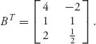
For this matrix v(BT) = 1, and we have a saddle point at row 1 column 2.
We conclude that the status quo point for this game is (E1, E2) = (![]() , 1) since that is the guaranteed payoff to each player without cooperation or negotiation. This means that any bargaining must begin with the guaranteed payoff pair (
, 1) since that is the guaranteed payoff to each player without cooperation or negotiation. This means that any bargaining must begin with the guaranteed payoff pair (![]() , 1). This cuts off the feasible set as in Figure 6.11.
, 1). This cuts off the feasible set as in Figure 6.11.
The new feasible set consists of the points in Figure 6.11 and to the right of the lines emanating from the security point (![]() , 1). It is like moving the origin to the new point (
, 1). It is like moving the origin to the new point (![]() , 1).
, 1).
Note that in this problem the Pareto-optimal boundary is the line connecting (1, 4) and (3, 1) because no player can get a bigger payoff on this line without forcing the other player to get a smaller payoff. A point in the set can’t go to the right and stay in the set without also going down; a point in the set can’t go up and stay in the set without also going to the left.
The question now is to find the cooperative, negotiated best payoff for each player. How does cooperation help? Well, suppose, for example, that the players agree to play as follows: I will play row I1 half the time and row I2 half the time as long as II plays column II1 half the time and column II2 half the time. This is not optimal for player II in terms of his safety level. But, if they agree to play this way, they will get ![]() (1, 4) +
(1, 4) + ![]() (3, 1) = (2,
(3, 1) = (2, ![]() ). So player I gets 2 >
). So player I gets 2 > ![]() and player II gets
and player II gets ![]() > 1, a big improvement for each player over his or her own individual safety level. So, they definitely have an incentive to cooperate.
> 1, a big improvement for each player over his or her own individual safety level. So, they definitely have an incentive to cooperate.
Example 6.23 Here is another example. The bimatrix is
The reader can calculate that the safety level is given by the point
![]()
and the optimal strategies that will give these values are XA = (![]() ,
, ![]() ), YA = (
), YA = (![]() ,
, ![]() ), and XB = (
), and XB = (![]() ,
, ![]() ), YB = (
), YB = (![]() ,
, ![]() ). Negotiations start from the safety point. Figure 6.12 shows the safety point and the associated feasible payoff pairs above and to the right of the dark lines.
). Negotiations start from the safety point. Figure 6.12 shows the safety point and the associated feasible payoff pairs above and to the right of the dark lines.
The shaded region in Figure 6.12 is the convex hull of the pure payoffs, namely, the feasible set, and is the set of all possible negotiated payoffs. The region of dot points is the set of noncooperative payoff pairs if we consider the use of all possible mixed strategies. The set we consider is the shaded region above and to the right of the safety point. It appears that a negotiated set of payoffs will benefit both players and will be on the line farthest to the right, which is the Pareto-optimal boundary. Player I would love to get (17, 2), while player II would love to get (2, 17). That probably won’t occur but they could negotiate a point along the line connecting these two points and compromise on obtaining, say, the midpoint
![]()
So they could negotiate to get 9.5 each if they agree that each player would use the pure strategies X = (1, 0) = Y half the time and play pure strategies X = (0, 1) = Y exactly half the time. They have an incentive to cooperate.
Now suppose that player II threatens player I by saying that she will always play strategy II1 unless I cooperates. Player II’s goal is to get the 17 if and when I plays I1, so I would receive 2. Of course, I does not have to play I1, but if he doesn’t, then I will get −19, and II will get −7. So, if I does not cooperate and II carries out her threat, they will both lose, but I will lose much more than II. Therefore, II is in a much stronger position than I in this game and can essentially force I to cooperate. This implies that the safety level of (−![]() , −
, −![]() ) loses its effect here because II has a credible threat that she can use to force player I to cooperate. This also seems to imply that maybe player II should expect to get more than 9.5 to reflect her stronger bargaining position from the start.
) loses its effect here because II has a credible threat that she can use to force player I to cooperate. This also seems to imply that maybe player II should expect to get more than 9.5 to reflect her stronger bargaining position from the start.
FIGURE 6.11 The reduced feasible set; safety at (![]() , 1).
, 1).
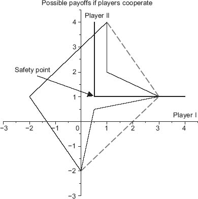
FIGURE 6.12 Achievable payoff pairs with cooperation; safety point = ![]()
![]() , −
, −![]()
![]() .
.
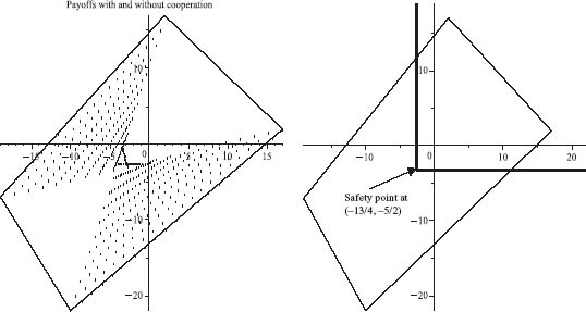
FIGURE 6.13 Pareto-optimal boundary is line connecting (2, 17) and (17, 2).
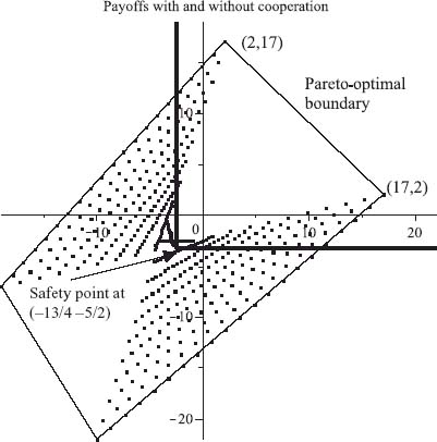
FIGURE 6.14 Bargaining solution where curves just touch Pareto boundary at (9.125, 9.875).
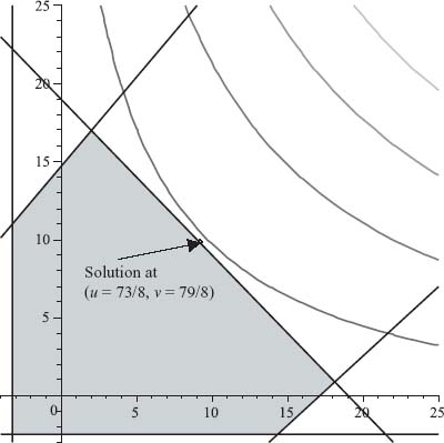
FIGURE 6.15 Security point ![]() −
−![]() , −
, −![]()
![]() , Pareto boundary v = −2u + 5, solution (1.208, 2.583).
, Pareto boundary v = −2u + 5, solution (1.208, 2.583).
The preceding example indicates that there may be a more realistic choice for a safety level than the values of the associated games, taking into account various threat possibilities. We will see later that this is indeed the case.
6.4.1 THE NASH MODEL WITH SECURITY POINT
We start with any old security status quo point (u*, v*) for a two-player cooperative game with matrices A, B. This leads to a feasible set of possible negotiated outcomes depending on the point we start from (u*, v*). This may be the safety point u* = value(A), v* = value(BT), or not. For any given such point and feasible set S, we are looking for a negotiated outcome, call it (![]() ,
, ![]() ). This point will depend on (u*, v*) and the set S, so we may write
). This point will depend on (u*, v*) and the set S, so we may write
![]()
The question is how to determine the point (![]() ,
, ![]() )? John Nash proposed the following requirements for the point to be a negotiated solution:
)? John Nash proposed the following requirements for the point to be a negotiated solution:
- Axiom 1. We must have
 ≥ u* and
  ≥ v*. Each player must get at least the status quo point.
 - Axiom 2. The point (, )
 S, that is, it must be a feasible point.
 - Axiom 3. If (u, v) is any point in S, so that u ≥ and v ≥ , then it must be the case that u = , v = . In other words, there is no other point in S, where both players receive more. This is Pareto-optimality.
- Axiom 4. If (, ) T
 S and (, ) = f(T, u*, v*) is the solution to the bargaining problem with feasible set T, then for the larger feasible set S, either (, ) = f(S, u*, v*) is the bargaining solution for S, or the actual bargaining solution for S is in S − T. We are assuming that the security point is the same for T and S. So, if we have more alternatives, the new negotiated position can’t be one of the old possibilities.
 - Axiom 5. If T is an affine transformation of S, T = a S + b =
 (S) and (, ) = f(S, u*, v*) is the bargaining solution of S with security point (u*, v*), then (a + b, a + b) = f(T, au* + b, av* + b) is the bargaining solution associated with T and security point (au* + b, av* + b). This says that the solution will not depend on the scale or units used in measuring payoffs.
 - Axiom 6. If the game is symmetric with respect to the players, then so is the bargaining solution. In other words, if (, ) = f(S, u*, v*) and (i) u* = v*, and (ii) (u, v) S ⇒ (v, u) S, then = . So, if the players are essentially interchangeable they should get the same negotiated payoff.
The amazing thing that Nash proved is that if we assume these axioms, there is one and only one solution of the bargaining problem. In addition, the theorem gives a constructive way of finding the bargaining solution.
Theorem 6.4.4 Let the set of feasible points for a bargaining game be nonempty and convex, and let (u*, v*) ![]() S be the security point. Consider the nonlinear programming problem
S be the security point. Consider the nonlinear programming problem
![]()
Assume that there is at least one point (u, v) ![]() S with u > u*, v > v*. Then there exists one and only one point (
S with u > u*, v > v*. Then there exists one and only one point (![]() ,
, ![]() )
) ![]() S that solves this problem, and this point is the unique solution of the bargaining problem (
S that solves this problem, and this point is the unique solution of the bargaining problem (![]() ,
, ![]() ) = f(S, u*, v*) that satisfies the axioms 1 − 6. If, in addition, the game satisfies the symmetry assumption, then the conclusion of axiom 6 tells us that
) = f(S, u*, v*) that satisfies the axioms 1 − 6. If, in addition, the game satisfies the symmetry assumption, then the conclusion of axiom 6 tells us that ![]() =
= ![]() .
.
Proof We will only sketch a part of the proof and skip the rest.
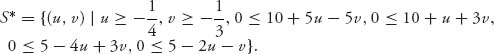
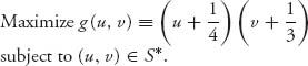
1. Existence. Define the function g(u, v) ≡ (u − u*)(v − v*). The set
![]()
is convex, closed, and bounded. Since g: S* → ![]() is continuous, a theorem of analysis (any continuous function on a closed and bounded set achieves a maximum and a minimum on the set) guarantees that g has a maximum at some point (
is continuous, a theorem of analysis (any continuous function on a closed and bounded set achieves a maximum and a minimum on the set) guarantees that g has a maximum at some point (![]() ,
, ![]() )
) ![]() S*. By assumption there is at least one feasible point with u > u*, v > v*. For this point g(u, v) > 0 and so the maximum of g over S* must be > 0 and therefore does not occur at the safety points u = u* or v = v*.
S*. By assumption there is at least one feasible point with u > u*, v > v*. For this point g(u, v) > 0 and so the maximum of g over S* must be > 0 and therefore does not occur at the safety points u = u* or v = v*.
2. Uniqueness. Suppose the maximum of g occurs at two points 0 < M = g(u′, v′) = g(u′′, v′′). If u′ = u′′, then
![]()
so that dividing out u′ − u*, implies that v′ = v′′ also. So we may as well assume that u′ < u′′ and that implies v′ > v′′ because (u′ − u*)(v′ − v*) = (u′′ − u*)(v′′ − v*) = M > 0 so that
![]()
Set (u, v) = ![]() (u′, v′) +
(u′, v′) + ![]() (u′′, v′′). Since S is convex, (u, v)
(u′′, v′′). Since S is convex, (u, v) ![]() S and u > u*, v > v*. So (u, v)
S and u > u*, v > v*. So (u, v) ![]() S*. Some simple algebra shows that
S*. Some simple algebra shows that
![]()
This contradicts the fact that (u′, v′) provides a maximum for g over S* and so the maximum point must be unique.
3. Pareto-optimality. We show that the solution of the nonlinear program, say, (![]() ,
, ![]() ), is Pareto-optimal. If it is not Pareto-optimal, then there must be another feasible point (u′, v′)
), is Pareto-optimal. If it is not Pareto-optimal, then there must be another feasible point (u′, v′) ![]() S for which either u′ >
S for which either u′ > ![]() and v′ ≥
and v′ ≥ ![]() , or v′ >
, or v′ > ![]() and u′ ≥
and u′ ≥ ![]() . We may as well assume the first possibility. Since
. We may as well assume the first possibility. Since ![]() > u*,
> u*, ![]() > v*, we then have u′ > u* and v′ > v* and so g(u′, v′) > 0. Next, we have
> v*, we then have u′ > u* and v′ > v* and so g(u′, v′) > 0. Next, we have
![]()
But this contradicts the fact that (![]() ,
, ![]() ) maximizes g over the feasible set. Hence, (
) maximizes g over the feasible set. Hence, (![]() ,
, ![]() ) is Pareto-optimal.
) is Pareto-optimal.
The rest of the proof will be skipped, and the interested reader can refer to the references, for example, the book by Jones (2000), for a complete proof. ![]()
Example 6.24 In an earlier example, we considered the game with bimatrix
The safety levels are u* = value(A) = −![]() , v* = value(BT) = −
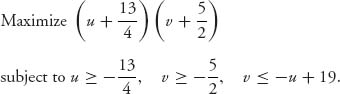
, v* = value(BT) = −![]() , Figure 6.13 for this problem shows the safety point and the associated feasible payoff pairs above and to the right. Now we need to describe the Pareto-optimal boundary of the feasible set. We need the equation of the lines forming the Pareto-optimal boundary. In this example, it is simply v = −u + 19, which is the line with negative slope to the right of the safety point. It is the only place where both players cannot simultaneously improve their payoffs. (If player I moves right, to stay in the feasible set player II must go down.)
, Figure 6.13 for this problem shows the safety point and the associated feasible payoff pairs above and to the right. Now we need to describe the Pareto-optimal boundary of the feasible set. We need the equation of the lines forming the Pareto-optimal boundary. In this example, it is simply v = −u + 19, which is the line with negative slope to the right of the safety point. It is the only place where both players cannot simultaneously improve their payoffs. (If player I moves right, to stay in the feasible set player II must go down.)
To find the bargaining solution for this problem, we have to solve the nonlinear programming problem:
The Maple commands used to solve this are as follows:
> with(Optimization):
> NLPSolve((u+13/4)*(v+5/2),
     u>=-13/4, v>=-5/2, v<=-u+19, maximize);
This gives the optimal bargained payoff pair (![]() =
= ![]() = 9.125,
= 9.125, ![]() =
= ![]() = 9.875). The maximum of g is g(
= 9.875). The maximum of g is g(![]() ,
, ![]() ) = 153.14, which we do not really use or need.
) = 153.14, which we do not really use or need.
The bargained payoff to player I is ![]() = 9.125 and the bargained payoff to player II is
= 9.125 and the bargained payoff to player II is ![]() = 9.875. We do not get the point we expected, namely, (9.5, 9.5); that is due to the fact that the security point is not symmetric. Player II has a small advantage.
= 9.875. We do not get the point we expected, namely, (9.5, 9.5); that is due to the fact that the security point is not symmetric. Player II has a small advantage.
You can see in the Figure 6.14 that the solution of the problem occurs just where the level curves, or contours of g are tangent to the boundary of the feasible set. Since the function g has concave up contours and the feasible set is convex, this must occur at exactly one point. Finally, knowing that the optimal point must occur on the Pareto-optimal boundary means we could solve the nonlinear programming problem by calculus. We want to maximize
![]()
This is an elementary calculus maximization problem.
Example 6.25 We will work through another example from scratch. We start with the following bimatrix:
1. Find the security point. To begin we find the values of the associated matrices
![]()
Then, value(A) = −![]() and value(BT) = −
and value(BT) = −![]() . Hence, the security point is (u*, v*) =
. Hence, the security point is (u*, v*) = ![]() −
−![]() , −
, −![]()
![]() .
.
2. Find the feasible set. The feasible set, taking into account the security point, is
3. Set up and solve the nonlinear programming problem. The nonlinear programming problem is then
Maple gives us the solution ![]() =
= ![]() = 1.208,
= 1.208, ![]() =
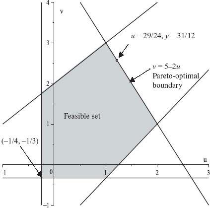
= ![]() = 2.583. If we look at Figure 6.15 for S*, we see that the Pareto-optimal boundary is the line v = −2u + 5, 1 ≤ u ≤ 2.
= 2.583. If we look at Figure 6.15 for S*, we see that the Pareto-optimal boundary is the line v = −2u + 5, 1 ≤ u ≤ 2.
The solution with the safety point given by the values of the zero sum games is at point (![]() ,
, ![]() ) = (1.208, 2.583). The conclusion is that with this security point, player I receives the negotiated solution
) = (1.208, 2.583). The conclusion is that with this security point, player I receives the negotiated solution ![]() = 1.208 and player II the amount
= 1.208 and player II the amount ![]() = 2.583. Again, we do not need Maple to solve this problem if we know the line where the maximum occurs, which here is v = −2u + 5, because then we may substitute into g and use calculus:
= 2.583. Again, we do not need Maple to solve this problem if we know the line where the maximum occurs, which here is v = −2u + 5, because then we may substitute into g and use calculus:
So this gives us the solution as well.
4. Find the strategies giving the negotiated solution. How should the players cooperate in order to achieve the bargained solutions we just obtained? To find out, the only points in the bimatrix that are of interest are the endpoints of the Pareto-optimal boundary, namely, (1, 3) and (2, 1). So the cooperation must be a linear combination of the strategies yielding these payoffs. Solve
![]()
to get λ = ![]() . This says that (I, II) must agree to play (row 1, column 1) with probability
. This says that (I, II) must agree to play (row 1, column 1) with probability ![]() and (row 2, column 2) with probability
and (row 2, column 2) with probability ![]() .
.
The Nash bargaining theorem also applies to games in which the players have payoff functions u1(x, y), u2(x, y), where x, y are in some interval and the players have a continuum of strategies. As long as the feasible set contains some security point u1*, u2*, we may apply Nash’s theorem. Here is an example.
Example 6.26 Suppose that two persons are given $1000, which they can split if they can agree on how to split it. If they cannot agree they each get nothing. One player is rich, so her payoff function is
![]()
because the receipt of more money will not mean that much. The other player is poor, so his payoff function is
![]()
because small amounts of money mean a lot but the money has less and less impact as he gets more but no more than $1000. We want to find the bargained solution. The safety points are taken as (0, 0) because that is what they get if they can’t agree on a split. The feasible set is S = {(x, y) | 0 ≤ x, y ≤ 1000, x + y ≤ 1000}.
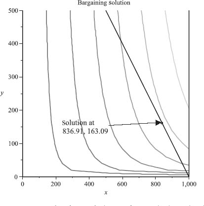
Figure 6.16 illustrates the feasible set and the contours of the objective function.
The Nash bargaining solution is given by solving the problem
![]()
subject to
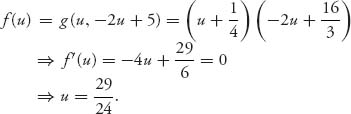
Since the solution will occur where x + y = 1000, substitute x = 1000 − y. If we take a derivative of f(y) = ![]() (1000 − y) ln(y + 1) and set to zero, we obtain that we have to solve the equation
(1000 − y) ln(y + 1) and set to zero, we obtain that we have to solve the equation ![]() which, with the aid of a calculator, is y = 163.09.
which, with the aid of a calculator, is y = 163.09.
The solution is obtained using Maple as follows.
> f:=(x, y)->(x/2)*(ln(1+y));
> cnst:=0<=x, x<=1000, 0 <=y, y<=1000, x+y <=1000;
> with(Optimization):
> NLPSolve(f(x, y), cnst, assume=nonnegative, maximize);
Maple tells us that the maximum is achieved at x = 836.91, y = 163.09, so the poor man gets $163 while the rich woman gets $837. The utility (or value of this money) to each player is u1 = 418.5 to the rich guy, and u2 = 5.10 to the poor guy. Figure 6.16 shows the feasible set as well as several level curves of f(x, y) = k. The optimal solution is obtained by increasing k until the curve is tangent to the Pareto-optimal boundary. That occurs here at the point (836.91, 163.09). The actual value of the maximum is of no interest to us.
6.4.2 THREATS
Negotiations of the type considered in the previous section do not take into account the relative strength of the positions of the players in the negotiations. As mentioned earlier, a player may be able to force the opposing player to play a certain strategy by threatening to use a strategy that will be very detrimental for the opponent. These types of threats will change the bargaining solution. Let’s start with an example.
FIGURE 6.16 Rich and poor split $1000: solution at (836.91, 163.09).
Example 6.27 We will consider the two-person game with bimatrix
Player I’s payoff matrix is
![]()
and for II
![]()
It is left to the reader to verify that value(A) = −![]() , value(BT) = −
, value(BT) = −![]() so the security point is (u*, v*) = (−
so the security point is (u*, v*) = (−![]() , −
, −![]() ).
).
With this security point, we solve the problem
In the usual way, we get the solution ![]() = 7.501,
= 7.501, ![]() = 1.937. This is achieved by players I and II agreeing to play the pure strategies (I1, II1) 31.2% of the time and pure strategies (I2, II2) 68.8% of the time. So with the safety levels as the value of the games, we get the bargained payoffs to each player as 7.501 to player I and 1.937 to player II. Figure 6.17 is a three-dimensional diagram of the contours of g(u, v) over the shaded feasible set. The dot shown on the Pareto boundary is the solution to our problem.
= 1.937. This is achieved by players I and II agreeing to play the pure strategies (I1, II1) 31.2% of the time and pure strategies (I2, II2) 68.8% of the time. So with the safety levels as the value of the games, we get the bargained payoffs to each player as 7.501 to player I and 1.937 to player II. Figure 6.17 is a three-dimensional diagram of the contours of g(u, v) over the shaded feasible set. The dot shown on the Pareto boundary is the solution to our problem.
The problem is that this solution is not realistic for this game. Why? The answer is that player II is actually in a much stronger position than player I. In fact, player II can threaten player I with always playing II1. If player II does that and player I plays I1, then I gets 2 < 7.501, but II gets 4 > 1.937. So, why would player I do that? Well, if player I instead plays I2, in order to avoid getting less, then player I actually gets −8, while player II gets −2. So both will lose, but I loses much more. Player II’s threat to always play II1, if player I doesn’t cooperate on II’s terms, is a credible and serious threat that player I cannot ignore. Next, we consider how to deal with this problem.
FIGURE 6.17 The feasible set and level curves in three dimensions. Solution is at (7.5, 1.93) for security point ![]() −
−![]() , −
, −![]()
![]() .
.
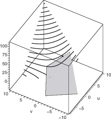
FIGURE 6.18 Feasible set with security point (−8, −2) using threat strategies.
6.4.2.1 Finding the Threat Strategies. In a threat game we replace the security levels (u*, v*), which we have so far taken to be the value of the associated games u* = value(A), v* = value(BT), with the expected payoffs to each player if threat strategies are used. Why do we focus on the security levels? The idea is that the players will threaten to use their threat strategies, say (Xt, Yt), and if they do not come to an agreement as to how to play the game, then they will use the threat strategies and obtain payoffs EI(Xt, Yt) and EII(Xt, Yt), respectively. This becomes their security point if they don’t reach an agreement.
In the Example 6.27, player II seemed to have a pure threat strategy. In general, both players will have a mixed threat strategy, and we have to find a way to determine them. For now, suppose that in the bimatrix game player I has a threat strategy Xt and player II has a threat strategy Yt. The new status quo or security point will be the expected payoffs to the players if they both use their threat strategies:
![]()
Then we return to the cooperative bargaining game and apply the same procedure as before but with the new threat security point; that is, we seek to
![]()
Note that we are not using BT for player II’s security point but the matrix B because we only need to use BT when we consider player II as the row maximizer and player I as the column minimizer.
In the Example 6.27, let’s suppose that the threat strategies are Xt = (0, 1) and Yt = (1, 0). Then the expected payoffs give us the safety point u* = XtT AYt = −8 and v* = Xt BYtT = −2 (see Figure 6.18). Changing to this security point increases the size of the feasible set and changes the objective function to g(u, v) = (u + 8)(v + 2).
When we solved this example with the security point (−![]() , −
, −![]() ), we obtained the payoffs 7.501 for player I and 1.937 for player II. The solution of the threat problem is
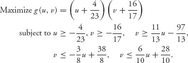
), we obtained the payoffs 7.501 for player I and 1.937 for player II. The solution of the threat problem is ![]() = 5 < 7.501,
= 5 < 7.501, ![]() = 2.875 > 1.937. This reflects the fact that player II has a credible threat and therefore should get more than if we ignore the threat.
= 2.875 > 1.937. This reflects the fact that player II has a credible threat and therefore should get more than if we ignore the threat.
The question now is how to pick the threat strategies? How do we know in the previous example that the threat strategies we chose were the best ones? We continue our example to see how to solve this problem. This method follows the procedure as presented by Jones (2000).
We look for a different security point associated with threats that we call the optimal threat security point. Let ut denote the payoff to player I if both players use their optimal threat strategies. Similarly, vt is the payoff to player II if they both play their optimal threat strategies. At this point, we don’t know what these payoffs are and we don’t know what the optimal threat strategies are, but (ut, vt) will be what they each get if their threats are carried out. This should be out threat security point.
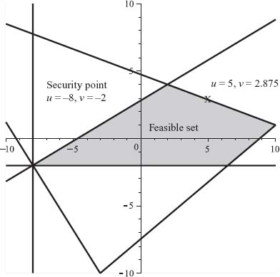
The Pareto-optimal boundary for our problem is the line segment v = −![]() u +
u + ![]() , 2 ≤ u ≤ 10. This line has slope mp = −
, 2 ≤ u ≤ 10. This line has slope mp = −![]() . Consider now a line with slope −mp =
. Consider now a line with slope −mp = ![]() through any possible threat security point in the feasible set (ut, vt). Referring to Figure 6.19, the line will intersect the Pareto-optimal boundary line segment at some possible negotiated solution (
through any possible threat security point in the feasible set (ut, vt). Referring to Figure 6.19, the line will intersect the Pareto-optimal boundary line segment at some possible negotiated solution (![]() ,
, ![]() ). The line with slope −mp through (ut, vt), whatever the point is, has the equation
). The line with slope −mp through (ut, vt), whatever the point is, has the equation
![]()
It is a fact (see Lemma 6.4.5) that this line must pass through the optimal threat security point.
FIGURE 6.19 Lines through possible threat security points.
The equation of the Pareto-optimal boundary line is
![]()
so the intersection point of the two lines will be at the coordinates
Now, remember that we are trying to find the best threat strategies to use, but the primary objective of the players is to maximize their payoffs ![]() ,
, ![]() . This tells us exactly what to do to find the optimal threat security point:
. This tells us exactly what to do to find the optimal threat security point:
- Player I will maximize if she chooses threat strategies to maximize the quantity −mp ut − vt =
 ut − vt.
 - Player II will maximize if he chooses threat strategies to minimize the same quantity −mp ut − vt because the Pareto-optimal boundary will have mp < 0, so the sign of the term multiplying ut will be opposite in and .
Putting these two goals together, it seems that we need to solve a game with some matrix. The rules following will show exactly what we need to do.
Summary Approach for Bargaining with Threat Strategies. Here is the general procedure for finding ut, vt and the optimal threat strategies as well as the solution of the bargaining game:
![]()
with matrix −mp A − B.
Alternatively, we may apply the nonlinear programming method with security point (ut, vt) to find (![]() ,
, ![]() ).
).
Example 6.27 (continued) Carrying out these steps for our example, mp = −![]() , b =
, b = ![]() , we find
, we find
We find value(![]() A − B) = −1 and, because there is a saddle point at the second row and first column, optimal threat strategies Xt = (0, 1), Yt = (1, 0). Then ut = Xt AYtT = −8, and vt = Xt BYtT = −2. Once we know that, we can use the formulas above to get
A − B) = −1 and, because there is a saddle point at the second row and first column, optimal threat strategies Xt = (0, 1), Yt = (1, 0). Then ut = Xt AYtT = −8, and vt = Xt BYtT = −2. Once we know that, we can use the formulas above to get
This matches with our previous solution in which we simply took the threat security point to be (−8, −2). Now we see that (−8, −2) is indeed the optimal threat security point.
Another Way to Derive the Threat Strategies Procedure. The preceding derivation leads to concise formulas for the bargained solution using optimal threat strategies. To further explain how this solution comes from the Nash bargaining theorem we apply it directly and justify the fact that the Pareto line, with slope mp, and the line through (![]() ,
, ![]() ) and (ut, vt), will have slope −mp.
) and (ut, vt), will have slope −mp.
Assume the Pareto-optimal set is the straight line segment
![]()
for some constants α, β, mp < 0, b. The negotiated payoffs should end up on P. Let Xt, Yt denote any (to be determined) threat strategies.
Let’s start by finding the optimal threat for player I. Nash proves that player I will get an eventual payoff u that maximizes the function
![]()
where we have used the fact that v = mp u + b. This function has a maximum in [α, β ]. Let’s assume it is an interior maximum so we can use calculus to find the critical point:
![]()
which, solving for u, gives us
![]()
Since f′′(u) = 2mp < 0, we know ![]() does provide a maximum of f. Since
does provide a maximum of f. Since ![]() = mp
= mp ![]() + b, we also get
+ b, we also get
Now we analyze the goals for each player. Player I wants to make ![]() , the payoff that player I should receive, as large as possible. This says, player I should choose Xt to maximize the term Xt(−mp A − B)YtT against all possible threats Yt for player II.
, the payoff that player I should receive, as large as possible. This says, player I should choose Xt to maximize the term Xt(−mp A − B)YtT against all possible threats Yt for player II.
From II’s point of view, player II wants ![]() also large as possible. Looking at the formula for
also large as possible. Looking at the formula for ![]() in (6.7) we see that player II, who controls the choice of Yt, will choose the threat strategy Yt so as to maximize −Xt(−mp A − B)YtT, which is equivalent to minimize Xt(−mp A − B)YtT against any threat Xt for player I.
in (6.7) we see that player II, who controls the choice of Yt, will choose the threat strategy Yt so as to maximize −Xt(−mp A − B)YtT, which is equivalent to minimize Xt(−mp A − B)YtT against any threat Xt for player I.
Once again we arrive at the problem that we must solve the zero sum matrix game with matrix −mp A − B. Von Neumann’s minimax theorem guarantees there is a value and saddle point for this game, denoted as (Xt, Yt) and they are the optimal threat strategies for each player in the original nonzero sum game.
Let value(−mp A − B) = Xt(−mp A − B)YtT denote the value of the game with matrix −mp A − B. The payoffs for the bargained solution will then be given by
Assuming that α < ![]() < β, we have completely solved the problem assuming we have an interior maximum α <
< β, we have completely solved the problem assuming we have an interior maximum α < ![]() < β .
< β .
The next lemma proves that if the Pareto-optimal boundary has slope mp, then the slope of the line through (ut = Xt AYtT, vt = Xt BYtT) and the bargaining solution (![]() ,
, ![]() ) must have slope −mp. This lemma is essential in seeing what happens if the Pareto-optimal boundary is not just a line segment but consists of several line segments.
) must have slope −mp. This lemma is essential in seeing what happens if the Pareto-optimal boundary is not just a line segment but consists of several line segments.
Lemma 6.4.5 If (![]() ,
, ![]() ) is the solution of the Nash bargaining problem with any security point (u0, v0) and the Pareto-optimal boundary through (
) is the solution of the Nash bargaining problem with any security point (u0, v0) and the Pareto-optimal boundary through (![]() ,
, ![]() ) is a straight line with slope mp and (
) is a straight line with slope mp and (![]() ,
, ![]() ) is not at an end point, then
) is not at an end point, then
![]()
That is, the slope of the line through (u0, v0) and (![]() ,
, ![]() ) must be the negative of the slope of the Pareto-optimal boundary at the point (
) must be the negative of the slope of the Pareto-optimal boundary at the point (![]() ,
, ![]() ).
).
Proof We have already seen that if ![]() is interior to (α, β) then (
is interior to (α, β) then (![]() ,
, ![]() ) by Nash’s theorem, maximizes f(u) = (u − u0)(mp u + b − v0). Taking the derivative and setting to zero we see that
) by Nash’s theorem, maximizes f(u) = (u − u0)(mp u + b − v0). Taking the derivative and setting to zero we see that
![]()
For arbitrary security point (u0, v0), the maximizing point is given by
![]()
Now we calculate the slope of the line through (u0, v0) and (![]() ,
, ![]() ):
):
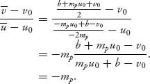
![]()
The preceding discussion gives us a general procedure to solve for the threat strategies. Note, however, that several things can make this procedure more complicated. First, the determination of the Pareto-optimal boundary of S is of critical importance. In Example 6.19, it consisted of only one line segment, but in practice there may be many such line segments and we have to work separately with each segment. That is because we need the slopes of the segments. This means that the threat strategies and the threat point ut, vt could change from segment to segment. An example below will illustrate this.
Another problem is that the Pareto-optimal boundary could be a point of intersection of two segments, so there is no slope for the point. Then, what do we do? The answer is that when we calculate the threat point (ut, vt) for each of the two line segments that intersect at a vertex, if this threat point is in the cone emanating from this vertex with the slopes shown in the Figure 6.20, then the threat solution of our problem is in fact at the vertex.
FIGURE 6.20 Bargaining solution for threats when threat point is in the cone is the vertex.
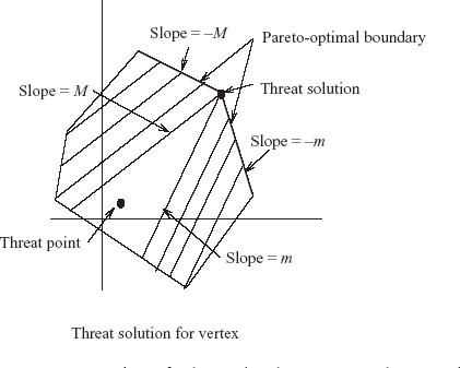
Example 6.28 Consider the cooperative game with bimatrix
| II1 | II2 | |
| I1 | (−1, −1) | (1, 1) |
| I2 | (2, −2) | (−2, 2) |
The individual matrices are as follows:
![]()
It is easy to calculate that value(A) = 0, value(BT) = 1 and so the status quo security point for this game is at (u*, v*) = (0, 1). The problem we then need to solve is
![]()
where
![]()
The solution of this problem is at the unique point (![]() ,
, ![]() ) = (
) = (![]() ,
, ![]() ), which you can see in the Figure 6.21.
), which you can see in the Figure 6.21.
Figure 6.21 was created with the following Maple commands:
> mypoints:=[[-1, -1], [-2, 2], [1, 1], [2, -2], [-1, -1]];
> constr:=0 <=x, -3*x-y<=4, x+3*y<=4, 3*x+y<=4, -x-3*y<=4, 1<=y;
> z:=(x+0)*(y-1);
> iplot2:=plots[inequal](constr, x=-0.5..2, y=-0.5..2,
    optionsfeasible=(color=white),
    optionsclosed=(color=black, thickness=2),
    optionsexcluded=(color=white), title=”Feasible Set
                                    with (0, 1) security”):
> pol:=plots[polygonplot](mypoints, color=yellow):
> cp:=plots[contourplot](z, x=-2..3, y=-2..3,
                           contours=40, axes=boxed, thickness=2):
> plots[display](iplot2, pol, cp);
The solution of the problem is given by the Maple commands:
> with(Optimization):
> NLPSolve(z, constr, maximize);
We get from these commands that z = 0.083, x = ![]() = 0.5, y =
= 0.5, y = ![]() = 1.167. As mentioned earlier, you may also get this by hand using calculus. You need to find the maximum of g(u, v) = u(v − 1) subject to u ≥ 0, v ≥ 1, and v = −
= 1.167. As mentioned earlier, you may also get this by hand using calculus. You need to find the maximum of g(u, v) = u(v − 1) subject to u ≥ 0, v ≥ 1, and v = −![]() +
+ ![]() . So, f(u) = g(u, v) = u(−
. So, f(u) = g(u, v) = u(−![]() +
+ ![]() ) is the function to maximize. Since f′(u) = −
) is the function to maximize. Since f′(u) = −![]() +
+ ![]() = 0 at u =
= 0 at u = ![]() ≥ 0, we have that
≥ 0, we have that ![]() =
= ![]() > 0,
> 0, ![]() =
= ![]() > 1 as our interior feasible maximum.
> 1 as our interior feasible maximum.
Next, to find the threat strategies we note that we have two possibilities because we have two line segments in Figure 6.21 as the Pareto-optimal boundary. We have to consider both mp = −![]() , b =
, b = ![]() and mp = −3, b = 4.
and mp = −3, b = 4.
Let’s use mp = −3, b = 4. We look for the value of the game with matrix 3A − B:
![]()
Then value (3A − B) = 0, and the optimal threat strategies are Xt = (![]() ,
, ![]() ) = Yt. Then the security threat points are as follows:
) = Yt. Then the security threat points are as follows:
![]()
This means that each player threatens to use (Xt, Yt) and receive 0 rather than cooperate and receive more.
Now the maximization problem becomes
![]()
where
![]()
The solution of this problem is at the unique point (![]() ,
, ![]() ) = (1, 1). You can see in Figure 6.22 how the level curves have bent over to touch at the vertex.
) = (1, 1). You can see in Figure 6.22 how the level curves have bent over to touch at the vertex.
What would have happened if we used the slope of the other line of the Pareto-optimal boundary? Let’s look at mp = −![]() , b =
, b = ![]() . The matrix is
. The matrix is
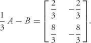
Then value (![]() A − B) = −
A − B) = −![]() , and the optimal threat strategies are Xt = (1, 0), Yt = (0, 1). The security threat points are as follows:
, and the optimal threat strategies are Xt = (1, 0), Yt = (0, 1). The security threat points are as follows:
![]()
This point is exactly the vertex of the feasible set.
Now the maximization problem becomes
![]()
where
![]()
But this set has exactly one point (as you should verify), and it is (1, 1), so we immediately get the solution (![]() = 1,
= 1, ![]() = 1), the same as what we got earlier.
= 1), the same as what we got earlier.
What happens if we try to use the formulas (6.6) for the threat problem? This question arises now because the contours of g are hitting the feasible set right at the point of intersection of two lines. The two lines have the equations
![]()
So, do we use mp = −3, b = 4, or mp = −![]() , b =
, b = ![]() ? Let’s calculate for both. For mp = −3, b = 4, ut = vt = 0, we have
? Let’s calculate for both. For mp = −3, b = 4, ut = vt = 0, we have
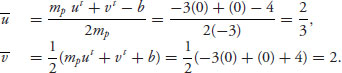
The point (![]() , 2) is not in St because (−
, 2) is not in St because (−![]() )(
)(![]() ) +
) + ![]() =
= ![]() < 2. So we no longer consider this point. However, because the point (ut, vt) = (0, 0) is inside the cone region formed by the lines through (1, 1) with slopes
< 2. So we no longer consider this point. However, because the point (ut, vt) = (0, 0) is inside the cone region formed by the lines through (1, 1) with slopes ![]() and 3, we know that the threat solution should be (1, 1).
and 3, we know that the threat solution should be (1, 1).
For mp = −![]() , b =
, b = ![]() , ut = vt = 1,
, ut = vt = 1,
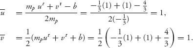
This gives (![]() = 1,
= 1, ![]() = 1), which is the correct solution.
= 1), which is the correct solution.
6.4.3 THE KALAI–SMORODINSKY BARGAINING SOLUTION
Nash’s bargaining solution does not always give realistic solutions because the axioms on which it is based may not be satisfied. The next example illustrates what can go wrong.
Example 6.29 At the risk of undermining your confidence, this example will show that the Nash bargaining solution can be totally unrealistic in an important problem. Suppose that there is a person, Moe, who has owes money to two creditors, Larry and Curly. He owes more than he can pay. Let’s say that he can pay at most $100 but he owes a total of $150 > $100 dollars, $90 to Curly and $60 to Larry. The question is how to divide the $100 among the two creditors. We set this up as a bargaining game and use Nash’s method to solve it.
First, the feasible set is
![]()
where u is the amount Larry gets, and v is the amount Curly will get.
The objective function we want to maximize at first is g(u, v) = uv because if Larry and Curly can’t agree on the split, then we assume that they each get nothing (because they have to sue and pay lawyers, etc.).
For the solution, we want to maximize g(u, v) subject to (u, v) ![]() S, u ≥ 0, v ≥ 0. It is straightforward to show that the maximum occurs at
S, u ≥ 0, v ≥ 0. It is straightforward to show that the maximum occurs at ![]() =
= ![]() = 50, as shown in Figure 6.23.
= 50, as shown in Figure 6.23.
In fact, if we take any safety point of the form u* = a = v*, we would get the exact same solution. This says that even though Moe owes Curly $90 and Larry $60, they both get the same amount as a settlement. That doesn’t seem reasonable, and I’m sure Curly would be very upset.
Now let’s modify the safety point to u* = −60 and v* = −90, which is still feasible and reflects the fact that the players actually lose the amount owed in the worst case, that is, when they are left holding the bag. This case is illustrated in Figure 6.24.
The solution is now obtained from maximizing g(u, v) = (u + 60)(v + 90) subject to (u, v) ![]() S, u ≥ −60, v ≥ −90, and results in
S, u ≥ −60, v ≥ −90, and results in ![]() = 60 and
= 60 and ![]() = 40. This is ridiculous because it says that Larry should be paid off in full while Curly, who is owed more, gets less than half of what he is owed.
= 40. This is ridiculous because it says that Larry should be paid off in full while Curly, who is owed more, gets less than half of what he is owed.
Of course, it is also possible to set this game up as a cooperative game and find the allocation. In this case, we take the characteristic function to be v(L) = 60, v(C) = 90, v(LC) = 100. Note that Moe is not a player in this game—he gives up the $100 no matter what. In this case, the least core is
![]()
The smallest ε so that C(ε) ≠ ![]() is ε1 = 25, and then we get C(25) = {(35, 65)} . The nucleolus solution is that Larry gets $35 and Curly gets $65. It is also easy to calculate that this is the same as the Shapley value.
is ε1 = 25, and then we get C(25) = {(35, 65)} . The nucleolus solution is that Larry gets $35 and Curly gets $65. It is also easy to calculate that this is the same as the Shapley value.
FIGURE 6.21 Security point (0, 1); cooperative solution (![]() =
= ![]() ,
, ![]() =
= ![]() ).
).
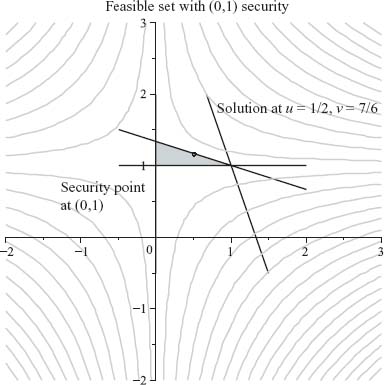
FIGURE 6.22 Security point (0, 0); cooperative solution (![]() = 1,
= 1, ![]() = 1).
= 1).
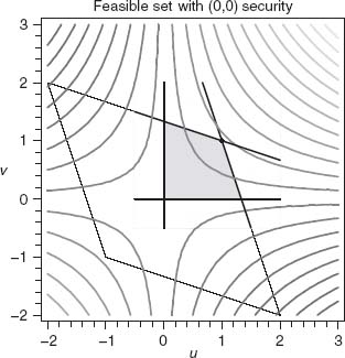
FIGURE 6.23 Moe pays both Curly and Larry $50 each.
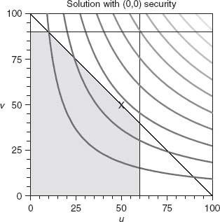
FIGURE 6.24 Moe pays Larry $60 and pays Curly $40.
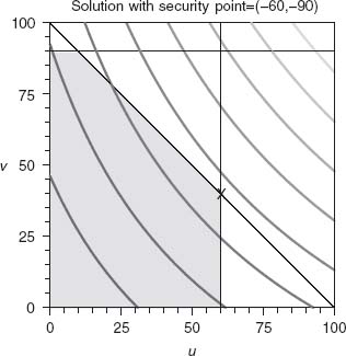
FIGURE 6.25 Two-stage bargaining.
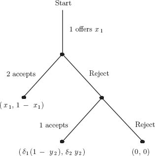
The problem with the Nash bargaining solution occurs whenever the players are not even close to being symmetric as in this example. In this case, there is an idea for solution due to Kalai and Smorodinsky (1975) that gives an alternate approach to solving the bargaining problem.
We will give a brief description of Kalai and Smorodinsky’s idea.10 The KS solution is based on the idea that each player should get an amount proportional to the player’s contribution. How to carry that out is given in the next steps:
![]()
Essentially, a is the maximum possible payoff for player I and b is the maximum possible payoff for player II.
(6.8)![]()
This line passes through (u*, v*) and (a, b), and is called the KS line, after Kalai and Smorodinsky.
For the Moe-Larry-Curly problem, with u* = −60, v* = −90, we calculate
![]()
This KS line will exit the feasible set where it crosses the line u + v = 100. This occurs at ![]() = 40, and so
= 40, and so ![]() = 60. Consequently, now Larry gets $40 and Curly gets $60. This is much more reasonable because almost everyone would agree that each creditor should be paid the same percentage of the amount Moe has as his percentage of the total owed. In this case 90/(90 + 60) =
= 60. Consequently, now Larry gets $40 and Curly gets $60. This is much more reasonable because almost everyone would agree that each creditor should be paid the same percentage of the amount Moe has as his percentage of the total owed. In this case 90/(90 + 60) = ![]() , so that Curly should get three-fifths of the $100 or $60. That is the KS solution as well.
, so that Curly should get three-fifths of the $100 or $60. That is the KS solution as well.
The KS solution gives another alternative for solution of the bargaining problem. However, it should be noted that the KS solution does not satisfy all the axioms for a desirable solution. In particular, it does not satisfy an economic axiom called the independence of irrelevant alternatives axiom.
6.4.4 SEQUENTIAL BARGAINING
In most bargaining situations, there are offers and counteroffers. Generally, this can go several rounds until an agreement is reached or negotiations break down. In this section, we will present a typical example to see how to analyze these problems.
It will be helpful to think about the problem in which there is a buyer and a seller. Player 1 is the buyer and player 2 is the seller. Suppose the item up for sale is a house.
Now suppose that the seller has a bottom line absolutely lowest price below which he will not sell the house. Let’s call that the reserve price. The seller offers the house for sale at a price called the ask price. The difference between the two prices is called the spread = asked−reserve. The spread is the negotiating range. Let x denote the fraction of the spread going to the buyer and 1 − x the fraction of the spread going to the seller. If we determine x, 0 ≤ x ≤ 1, the buyer and seller will have settled on a price and the transaction will take place at price reserve + (1 − x) spread.
In a one shot bargaining problem, the buyer and seller are aware of the reserve price and the ask price and the offer from the buyer is a take-it-or-leave-it deal. Let’s solve this problem for the one shot bargain.
We take the payoff for each player as
![]()
which is the fraction of the spread going to each player. Each player wants to make his fraction as large as possible. Let’s take any safety point (d1, d2) that determines the worth to each player if no deal is made.
The Nash bargaining problem then consists of maximizing
![]()
The solution is
![]()
and this works as long as |d1 − d2| ≤ 1. Note that if d1 = d2, the optimal split is ![]() , so the transaction takes place at the midpoint of the spread.
, so the transaction takes place at the midpoint of the spread.
To contrast this with the KS solution, we first calculate
![]()
and the KS line with security point (d1, d2), 0 ≤ di < 1, is ![]() . This line intersects the boundary of the feasible set x + y = 1 when
. This line intersects the boundary of the feasible set x + y = 1 when
![]()
When d1 = d2 = 0, the split is at the midpoint of the spread.
Now consider what happens if sequential bargaining is possible. Player 1 begins by offering the split at 1 − x. Player 2 then can choose to either accept the split or reject it. Then player 1 can accept or reject that. This can go on presumably forever. What prevents it from endlessly going through offer-counter offer is the time value of money. Let r > 0 and ![]() . Then r represents the interest rate on money and δ is the discount rate. What that means is that $1 today is worth $1(1 + r) in the next period, conversely, $1 in the next period is worth $1δ today. We assume that each player has their own discount rate δ1, δ2 if we think of the discount rate as representing a discount one will offer today to make the deal now.
. Then r represents the interest rate on money and δ is the discount rate. What that means is that $1 today is worth $1(1 + r) in the next period, conversely, $1 in the next period is worth $1δ today. We assume that each player has their own discount rate δ1, δ2 if we think of the discount rate as representing a discount one will offer today to make the deal now.
The payoff functions for each player are now given by

Let’s consider the two-stage bargaining problem. Consider Figure 6.25.
The game begins with an offer x1 from player 1. Player 2 may accept or reject the offer. If it is accepted, the game is over and player 1 gets x1, player 2 gets 1 − x1. If the first offer by player 1 is rejected, player 2 makes a counter offer y2 ![]() [0, 1]. If player 1 rejects the counter offer the game is over, no deal is reached, and the payoffs are 0 to each player. If player 1 accepts the offer, the game ends and the payoff to player 1 is δ1(1 − y2), while the payoff to player 2 is δ2y2.
[0, 1]. If player 1 rejects the counter offer the game is over, no deal is reached, and the payoffs are 0 to each player. If player 1 accepts the offer, the game ends and the payoff to player 1 is δ1(1 − y2), while the payoff to player 2 is δ2y2.
This is an extensive game with perfect information and can be solved by looking for a subgame perfect equilibrium via backward induction. Starting at the end of the second period, player 1 makes the final decision. If δ1(1 − y2) > 0, that is, if y2 ≠ 1, then player 1 receives the larger payoff δ1(1 − y2). Naturally, player 2 will choose y2 extremely close to 1 since 2 knows that any y2 < 1 will give 1 a positive payoff. Thus at the beginning of the last stage where player 2 offers y2 ≈ 1, player 2 gets ≈ δ2 and player 1 gets ≈ 0 (but positive).
Player 2, at the start of the first stage, will compare 1 − x1 with δ2 y2. If 1 − x1 > δ2 y2 ≈ δ2, player 2 will accept player 1’s first offer. Player 1’s offer needs to satisfy x1 < 1 − δ2, but as large as possible. That means player 1 will play x1 = 1 − δ2, and that should be the offer 1 makes at the start of the game.
So here is the result giving the subgame perfect equilibrium for each player:
- Player 1 begins the game by offering x1 = 1 − δ2. Then, if player 2 accepts the offer, the payoff to 1 is 1 − δ2 and the payoff to 2 is δ2. If player 2 rejects and counter offers y2 ≈ 1, y2 < 1, then player 1 will accept the offer, receiving δ1(1 − y2) > 0. If player 2 counters with y2 = 1, then player 1 is indifferent between acceptance or rejection (and so will reject).
Now let’s analyze the bargaining game with 3 rounds in Figure 6.26. To simplify the details we will assume that both players have the same discount factor δ = δ1 = δ2.
FIGURE 6.26 Three-stage bargaining.
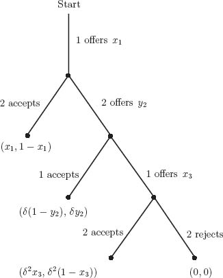
As before, player 1 begins by offering to take the fraction x1 of the spread, and 2 is left with 1 − x1 if 2 accepts. If 2 rejects 1’s offer, then 2 counters with an offer of y2 ![]() [0, 1], and 1 − y2 for player 1. Finally, player 1 may either accept player 2’s offer and the game ends, or reject the offer and counter with an offer of x3 for player 1, and 1 − x3 for player 2. Taking into account the discount factor δ, the payoffs are as follows:
[0, 1], and 1 − y2 for player 1. Finally, player 1 may either accept player 2’s offer and the game ends, or reject the offer and counter with an offer of x3 for player 1, and 1 − x3 for player 2. Taking into account the discount factor δ, the payoffs are as follows:
Now let’s calculate the subgame perfect equilibrium using backward induction:
What happens if this game can continue possibly forever? Well, we can figure that out by what we have already calculated. First, we need to make a change in the three-stage game if the final offer is rejected. Instead of (0, 0) going to each player, let s denote the total spread available and assume that when player 2 rejects player 1’s counter at stage 3, the payoff to each player is (δ2 s, δ2(1 − s)). We go through the analysis again.
Player 2 in stage 3 will accept the counter of player 1, x3, if δ2(1 − x3) ≥ δ2(1 − s), which is true if x3 ≤ s. Since player 1 gets δ2 x3 if the offer is accepted, player 1 makes the offer x3 as large as possible and so x3* = s.
Working back to the second stage, player 2’s offer of y2 will be accepted if δ(1 − y2) ≥ δ2 s, that is, if y2 ≤ 1 − δs. Since player 2 receives δy2, player 2 wants y2 to be as large as possible and hence offers y2 = 1 − δs in the second stage.
In the first stage, player 2 will accept player 1’s offer of x1 if 1 − x1 > δy2 = δ(1 − δs). Simplifying, this requires x1 < 1 − δ(1 − δs), or, making x1 as large as possible, player 1 should offer x1 = 1 − δ + δ2s in the first stage.
We may summarize the subgame perfect equilibrium by writing this down in reverse order.
| Player 1 | Player 2 |
| 1. Offer player 2 x1 = 1 − δ + δ2s. | 1. Accept if x1 = 1 − δ + δ2s. |
| 2. If player 2 offers y2 = 1 − δs, accept. | 2. Offer y2 = 1 − δs. |
| 3. Offer x3 = s. | 3. Accept if x3 = s. |
What should s be? If the bargaining goes on for three-stages and ends, s is 0 if no agreement can be achieved. In theory, the bargaining can go back and forth for quite a long time. The way to choose s is to observe that when we are in a three-stage game, at the third stage we are back to the original conditions at the start of the game for both players except for the fact that time has elapsed. In other words, player 1 will now begin bargaining just as she did in the beginning of the game. That implies that for the original three-stage game, s should be chosen so that the offer at the first stage x1 is the same as what she should offer at stage 3. This results in
![]()
Remark It may make more sense in many sequential bargaining problems to view the discount factor not as the time value of money, but as the probability the bargaining problem will end with a rejection of the latest offer. This would make δ very subjective, which is often the case with bargaining. In particular, when you are negotiating to buy a car, or house, you have to assess the chances that an offer will be rejected, and with no possibility of revisiting the offer. The next example illustrates this.
Example 6.30 Suppose you want to sell your car. You know it is worth at least $2000 and won’t take a penny under that. On the other hand, you really want to unload the car so you advertise it for sale at $2800. The market for your used car is not very good but eventually a buyer shows up. The buyer looks like he will give an offer but may not negotiate if the offer is turned down. The buyer thinks the same of you but he knows the car is worth at least $2000. Let’s take δ = 0.5 to account for the uncertainty in the continuation of bargaining. In this case, assuming indefinite stages of bargaining, the buyer should offer
![]()
and the seller should accept this offer.
Problems
6.57 A British game show involves a final prize. The two contestants may each choose either to Split the prize, or Claim the prize. If they Split the prize, they each get ![]() ; if they each Claim the prize, they each get 0. If one player Splits, and the other player Claims, the player who Claims the prize gets 1 and the other player gets 0. The game matrix is
; if they each Claim the prize, they each get 0. If one player Splits, and the other player Claims, the player who Claims the prize gets 1 and the other player gets 0. The game matrix is
![]()
6.58 Find the solution to the Nash bargaining problem for the game
![]()
6.59 Find the Nash bargaining solution, the threat solution, and the KS solution to the battle of the sexes game with matrix
![]()
Compare the solutions with the solution obtained using the characteristic function approach.
6.60 Find the Nash bargaining solution and the threat solution to the game with bimatrix
![]()
Find the KS line and solution.
6.61 Find the Nash bargaining solution and the threat solution to the game with bimatrix
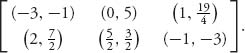
Find the KS line and solution.
6.62 Consider the sequential bargaining problem. Suppose that each player has their own discount factor δ1, δ2, 0 < δi < 1. Find the subgame perfect equilibrium for each player assuming the bargaining has three-stages and ends, as well as assuming the stages could continue forever.
6.63 You want to buy a seller’s condo. You look up what the seller paid for the condo 2 years ago and find that she paid $305, 000. You figure that she will absolutely not sell below this price. The seller has listed the condo at $350, 000. Assume that the sequential bargaining problem will go at most 3 rounds before everyone is fed up with the process and the deal falls apart. Take the discount factors for each player to be δ = 0.99. What should the offers be at each stage? What if the process could go on indefinitely?
6.64 The Nash solution also applies to payoff functions with a continuum of strategies. For example, suppose that two investors are bargaining over a piece of real estate and they have payoff functions u(x, y) = x + y, while v(x, y) = x + ![]() , with x, y ≥ 0, and x + y ≤ 1. Both investors want to maximize their own payoffs. The bargaining solution with safety point u* = 0, v* = 0 (because both players get zero if negotiations break down) is given by the solution of the problem
, with x, y ≥ 0, and x + y ≤ 1. Both investors want to maximize their own payoffs. The bargaining solution with safety point u* = 0, v* = 0 (because both players get zero if negotiations break down) is given by the solution of the problem
![]()
Solve this problem to find the Nash bargaining solution.
6.65 A classic bargaining problem involves a union and management in contract negotiations. If management hires w ≥ 0 workers, the company produces f(w) revenue units, where f is a continuous, increasing function. The maximum number of workers who are represented by the union is W. A person who is not employed by the company gets a payoff p0 ≥ 0, which is either unemployment benefits or the pay at another job. In negotiations with the union, the firm agrees to the pay level p and to employ 0 ≤ w ≤ W workers. We may consider the payoff functions as
![]()
and
![]()
Assume the safety security point is u* = 0 for the company and v* = Wp0 for the union.
![]()
Review Problems
True or False or Fill in the Blank or Complete the Statement.
6.66 A Nash equilibrium in a zero sum game is not the same as a saddle point.
6.67 The least core is always nonempty.
6.68 If the least core has only one allocation then that allocation is fair in the sense that it minimizes ….
6.69 In order for v(S) to be a characteristic function it must satisfy three conditions. What are they?
6.70 In order for a vector ![]() = (x1, …, xn) to be an imputation it must satisfy two conditions. What are they?
= (x1, …, xn) to be an imputation it must satisfy two conditions. What are they?
6.71 In order for a pair of strategies X*, Y* to be a Nash equilibrium for the game (A, B) it must satisfy two conditions. What are they?
6.72 The core of a cooperative game is the set ….
6.73 Is the following statement correct? If not, correct it. Equality of Payoffs in a two-person nonzero sum game says that EI(i, Y*) = EI(j, Y*) for all rows i, j if (X*, Y*) is a NE.
6.74 In the Nash bargaining solution, the problem reduces to
![]()
6.75 The Pareto-optimal boundary must have a negative slope because ….
6.76 The optimal threat strategies (Xt, Yt) in the Nash bargaining solution are given as the saddle point for the zero sum game with matrix −mp A − B, where mp is … .
6.5 Maple/Mathematica
6.5.1 FINDING THE NUCLEOLUS ONE STEP AT A TIME
Example 6.31 In this example, we will give the Maple commands at each stage to find the nucleolus. This entire procedure can be automated, but that is a programming problem.
We take the characteristic function
![]()
and this is in normalized form. We see that ![]() +
+ ![]() +
+ ![]() < 2, and so the core of the game C(0) is not empty by Proposition 6.1.7. We need to find the allocation within the core which solves our problem.11
< 2, and so the core of the game C(0) is not empty by Proposition 6.1.7. We need to find the allocation within the core which solves our problem.11
1. First linear programming problem. We start with the full set of possible coalitions excluding the grand coalition N and ![]() : Σ0 = {1, 2, 3, 12, 13, 23}. In addition, with the given characteristic function, we get the excesses
: Σ0 = {1, 2, 3, 12, 13, 23}. In addition, with the given characteristic function, we get the excesses
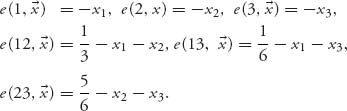
The Maple commands that give the solution are as follows:
> with(simplex):v1:=0:v2:=0:v3:=0:v12:=1/3:v13:=1/6:
                v23:=5/6:v123:=1;			1
> cnsts:=v1-x1<=z, v2-x2<=z, v3-x3<=z, v12-(x1+x2)<=z,
           v13-(x1+x3)<=z, v23-(x2+x3)<=z, x1+x2+x3=v123;
> minimize(z, cnsts);
Maple gives the solution ε1 = z = −![]() , x1 =
, x1 = ![]() , x2 =
, x2 = ![]() , x3 =
, x3 = ![]() . So this gives the allocation
. So this gives the allocation ![]() =
= ![]()
![]() ,
, ![]() ,
, ![]()
![]() . But this is not necessarily the unique allocation and therefore the solution to our game.
. But this is not necessarily the unique allocation and therefore the solution to our game.
To see if there are more allocations in X1, substitute z = −![]() as well as x3 = 1 − x1 − x2 in the constraint set. To do that in Maple use the substitute command
as well as x3 = 1 − x1 − x2 in the constraint set. To do that in Maple use the substitute command
> fcnsts:=subs(z=-1/12, x1=1-x2-x3, cnsts);
This will put the new constraint set into the variable fcnsts and gives us the output
fcnsts=1=1, x3 <= 7/12, -x2 <= -1/12, -x3 <= -1/12,
             -x2-x3 <= -11/12, x2+x3 <= 11/12, x2 <= 3/4.
To get rid of the first equality so that we can continue, use
> gcnsts:=fcnsts[2..7];
This puts the second through seventh elements of fcnsts into gcnsts. Now, to see if there are other solutions, we need to solve the system of inequalities in gcnsts for x1, x2. Maple does that as follows:
> with(SolveTools:-Inequality):
> glc:=LinearMultivariateSystem(gcnsts, [x2, x3]);
Maple solves the system of inequalities in the sense that it reduces the inequalities to simplest form and gives the following output:
x2 <=3/4, 1/3<=x2 x3<=-x2+11/12, -x2+11/12<=x3.
We see that ![]() ≤ x2 ≤
≤ x2 ≤ ![]() , x2 + x3 =
, x2 + x3 = ![]() and x1 =
and x1 = ![]() .
.
2. To get the second linear program, we first, have to see which coalitions are dropped. First, we assign the variables that are known from the first linear program and recalculate the constraints:
> assign(x1=1/12, z=-1/12);
> cnsts1:=v1-x1<=z, v2-x2<=z, v3-x3<=z, v12-(x1+x2)<=z,
           v13-(x1+x3)<=z, v23-(x2+x3)<=z, x1+x2+x3=v123;
Maple gives the output:
cnsts1:=-x3 <= -1/12, -x2-x3<=-11/12, -x2 <=-1/12, -x2 <= -1/3,
-1/12 <= -1/12, -x3 <=-1/6, 1/12+x2+x3=1.
Getting rid of the coalitions that have excess= −![]() (indicated by the output without any x variables), we have the new constraint set
(indicated by the output without any x variables), we have the new constraint set
> cnsts2:=v2-x2<=z2, v3-x3<=z2, v12-(x1+x2)<=z2,
              v13-(x1+x3)<=z2, x1+x2+x3=v123;
Now we solve the second linear program
> minimize(z2, cnsts2);
which gives
![]()
At each stage we need to determine whether there is more than one solution of the linear programming problem. To do that, we have to substitute our solution for z2 into the constraints and solve the inequalities:
> fcnsts2:=subs(z2=-7/24, 11/12=x2+x3, cnsts2);
> gcnsts2:=fcnsts2[2..5] union
                    {x2+x3<=11/12, x2+x3>=11/12};
> g1c2:=LinearMultivariateSystem(gcnsts2, [x2, x3]);
We get
glc2:=x2=13/24, x3 <= x2+x3=11/12,
and we know now that x1 = ![]() , x2 =
, x2 = ![]() , and x3 =
, and x3 = ![]() because x2 + x3 =
because x2 + x3 = ![]() .
.
We could continue setting up linear programs until we get the set of empty coalitions, but there is no point to that when we are doing it by hand (or with a Maple assist), because we are now at the point when we have one and only one allocation.
So we are finally done, and we conclude that
![]()
The first ε1 = −![]() and the second ε2 = −
and the second ε2 = −![]() .
.
Example 6.32 Three cities are to be connected to a water tower at a central location. Label the three cities 1, 2, 3 and the water tower as 0. The cost to lay pipe connecting location i with location j is denoted as cij, i ≠ j. Figure 6.27 contains the data for our problem.
The characteristic function is
![]()
This example was solved in the text using the exact formulas. Here is a Maple solution.
We will find the nucleolus of this game. First, the core of the game is illustrated in Figure 6.28.
This is clearly a nonempty set with many points, so we need to find the nucleolus. This is the complete set of Maple commands needed to do this:
> restart:with(simplex):v1:=0:v2:=0:v3:=0:
                        v12:=2:v13:=2:v23:=10:v123:=12;
> with(SolveTools:-Inequality):
> cnsts:={v1-x1<=z, v2-x2<=z, v3-x3<=z, v12-(x1+x2)<=z,
             v13-(x1+x3)<=z, v23-(x2+x3)<=z, x1+x2+x3=v123};
> minimize(z, cnsts);
> fcnsts:=subs(z=-1, x3=12-x1-x2, cnsts);
> gcnsts:=fcnsts[1..7] minus {fcnsts[2]};
> Core1:=subs(z=0, x3=12-x1-x2, cnsts);
> Core:=Core1 minus {Core1[1]};#This is needed to get rid of all
                               #equalities in Core1

> with(plots):#The next command plots the core.
> inequal(Core, x1=0..12, x2=0..12,
    optionsfeasible=(color=red),
    optionsopen=(color=blue, thickness=2),
    optionsclosed=(color=green, thickness=3),
    optionsexcluded=(color=yellow), labels=[x1, x2]);
    > # Now we set up for the next least core.
> g1c:=LinearMultivariateSystem(gcnsts, [x1, x2]);
> assign(x1=1, z=-1);
> cnsts1:={v1-x1<=z, v2-x2<=z, v3-x3<=z, v12-(x1+x2)<=z,
               v13-(x1+x3)<=z, v23-(x2+x3)<=z, x1+x2+x3=v123};

> cnsts2:={v2-x2<=z2, v3-x3<=z2, v13-(x1+x3)<=z2,
               v12-(x1+x2)<=z2, x1+x2+x3=v123};
> minimize(z2, cnsts2); #This command results in z2=-9/2
                          for the second least core.
> fcnsts2:=subs(z2=-9/2, cnsts2);
> gcnsts2:=fcnsts2[2..4] union {x2+x3<=11, x2+x3>=11};#Needed to
                     #convert equality to inequality
> # We now see if the second least core has more than one point.
> g1c2:=LinearMultivariateSystem(gcnsts2, [x2, x3]);
> assign(x2=11-x3, z2=-9/2);
> cnsts3:={v2-x2<=z2, v3-x3<=z2, v12-(x1+x2)<=z2,
            v13-(x1+x3)<=z2, x1+x2+x3=v123};
When we get to the last execution group, we have already determined that x1 = 1, x2 + x3 = 11, and the last constraint set gives
cnst3={12 = 12, -x3 <= -9/2, -x3 <= -11/2, x3 <= 13/2, x3 <= 11/2},
which tells us that x3 = ![]() and x2 = 11 −
and x2 = 11 − ![]() =
= ![]() . We have found that the nucleolus consists of the single allocation
. We have found that the nucleolus consists of the single allocation
![]()
6.5.2 MATHEMATICA CODE FOR THREE-PERSON NUCLEOLUS
FIGURE 6.27 Three cities and a water tower.
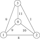
FIGURE 6.28 Core of three-city problem.
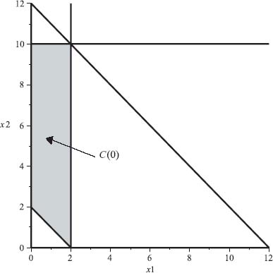
First, we need to check if the core is empty to see if we can use the formulas. The first snippet actually finds the least ε = ε1 for the least core.
Clear["Global'*"]

(*  This  program  implements  the  theorem  with  explicit  formulas  for
3-person games*)
(*  If  the  returned  value  of  z  is  <0,   the  core  is  nonempty;  if  z>0
then the core is empty*)

IsCoreEmpty[v1_, v2_, v3_, v12_, v13_, v23_, v123_] :=
 Module[{x1, x2, x3}, obj = z;
  cnsts = {v1 - x1 <= z, v2 - x2 <= z, v3 - x3 <= z,
    v12 - x1 - x2 <= z, v13 - x1 - x3 <= z, v23 - x2 - x3 <= z,
    x1 + x2 + x3 == v123}; Minimize[{obj, cnsts}, {x1, x2, x3}]]
For example, suppose v(i) = 0, v(12) = 100, v(13) = 0, v(23) = 100, v(123) = 200. The command is:
IsCoreEmpty[0, 0, 0, 100, 0, 100, 200]
(* This produces z=-50 so C(0) not empty *)
If we take v(i) = 0, v(12) = v(13) = v(23) = v(123) = 1, the command is:
IsCoreEmpty[0, 0, 0, 1, 1, 1, 1]

(* This produces z=1/3 so C(0)= empty *)
Assuming the condition C(0) ≠ ![]() the following code (due to Leng and Parlar (2010) in Maple) will quickly check the conditions of the theorem, print which case holds, and compute the nucleolus.
the following code (due to Leng and Parlar (2010) in Maple) will quickly check the conditions of the theorem, print which case holds, and compute the nucleolus.
CheckCore[v12_, v13_, v23_, v123_] :=
 Module[{y1, y2, y3},
  Which [v123 >= 3*v12 && v123 >= 3*v13 && v123 >= 3*v23,
   {y1 = v123/3, y2 = y1, y3 = y1,
    Print["Case 1"]},
    v123 >= v12 + 2*v23 && v123 >= v12 + 2*v13 && v123 <= 3*v12,
    {y1 = (v123 + v12)/4,
    y2 = y1,
    y3 = (v123 - v12)/2,
    Print["Case 2"]},
    v123 >= v12 + 2*v23 && v123 <= v12 + 2*v13 && v12 >= v13,
    {y1 = (v12 + v13)/2,
    y2 = (v123 - v13)/2,
    y3 = (v123 - v12)/2,
    Print["Case 3"]},
    v123 <= v12 + 2*v23 && v123 >= v12 + 2*v13 && v23 <= v12,
    {y1 = (v123 - v23)/2,
    y2 = (v12 + v23)/2,
    y3 = (v123 - v12)/2,
    Print["Case 4"]},
    v123 <= v12 + 2*v23 && v123 <= v12 + 2*v13 &&
    v123 + v12 >= 2*(v13 + v23),
    {y1 = (v123 + v12 - 2*(v23 - v13))/4,
    y2 = (v123 + v12 + 2*(v23 - v13))/4,
    y3 = (v123 - v12)/2,
    Print["Case 5"]},
    v123 >= v13 + 2*v23 && v123 >= v13 + 2*v12 && v123 <= 3*v13 ,
    {y1 = (v123 + v13)/4,
    y2 = (v123 - v13)/2,
    y3 = y1,
    Print["Case 6"]},
    v123 >= v13 + 2*v23 && v123 <= v13 + 2*v12 && v13 >= v12,
    {y1 = (v12 + v13)/2,
    y2 = (v123 - v13)/2,
    y3 = (v123 - v12)/2,
    Print["Case 7"]},
    v123 <= v13 + 2*v23 && v123 >= v13 + 2*v12 && v13 >= v23,
    {y1 = (v123 - v23)/2,
    y2 = (v123 - v13)/2,
    y3 = (v13 + v23)/2,
    Print["Case 8"]},
    v123 <= v13 + 2*v23 && v123 <= v13 + 2*v12 &&
    v123 + v13 >= 2*(v12 + v23),
    {y1 = (v123 + v13 - 2*(v23 - v12))/4,
    y2 = (v123 - v13)/2,
    y3 = (v123 + v13 + 2*(v23 - v12))/4,
    Print["Case 9"]},
    v123 >= v23 + 2*v13 && v123 >= v23 + 2*v12 && v123 <= 3*v23 ,
    {y1 = (v123 - v23)/2,
    y2 = (v123 + v23)/4,
    y3 = y2,
    Print["Case 10"]},
    v123 >= v23 + 2*v13 && v123 <= v23 + 2*v12 && v23 >= v12,
    {y1 = (v123 - v23)/2,
    y2 = (v12 + v23)/2,
    y3 = (v123 - v12)/2,
    Print["Case 11"]},
    v123 <= v23 + 2*v13 && v123 >= v23 + 2*v12 && v23 >= v13,
    {y1 = (v123 - v23)/2,
    y2 = (v123 - v13)/2,
    y3 = (v13 + v23)/2,
    Print["Case 12"]},
    v123 <= v23 + 2*v13 && v123 <= v23 + 2*v12 &&
    v123 + v23 >= 2*(v13 + v12),
    {y1 = (v123 - v23)/2,
    y2 = (v123 + v23 - 2*(v13 - v12))/4,
    y3 = (v123 + v23 + 2*(v13 - v12))/4,
    Print["Case 13"]},
    v123 + v12 <= 2*(v13 + v23) && v123 + v13 <= 2*(v12 + v23) &&
    v123 + v23 <= 2*(v13 + v12),
    {y1 = (v123 + v12 + v13 - 2*v23)/3,
    y2 = (v123 + v12 + v23 - 2*v13)/3,
    y3 = (v123 + v13 + v23 - 2*v12)/3,
    Print["Case 14"]}
    ]
  ]
For example, the command CheckCore[100, 0, 100, 200] produces the output
Case 4, x_1=50, x_2=100, x_3=50.
6.5.3 THE SHAPLEY VALUE WITH MAPLE
The following Maple commands can be used to calculate the Shapley value of a cooperative game. All you need to do is to let S be the set of numbered players, and define the characteristic function as v. The list M = [M[k]] consists of all the possible coalitions.
>restart:with(combinat):S:={1, 2, 3, 4};
>L:=powerset(S):M:=convert(L, list):M:=sort(M, length);K:=nops(L);
># Define the characteristic function
>for  k  from  1  to  K  do  if  nops(M[k])<=1  then  v(M[k]):=0;  end  if; end  do;
v({1, 2}):=0:v({1, 3}):=0:v({2, 3}):=0:v({1, 4}):=5:v({2, 4}):=10:
v({3, 4}):=0:
v({1, 2, 3}):=0:v({1, 3, 4}):=25:v({2, 3, 4}):=30:v({1, 2, 4}):=35:
v({1, 2, 3, 4}):=55:
># Calculate Shapley
> for i from 1 to nops(S) do
  x[i]:=0:
     for k from 1 to K do
        if member(i, M[k]) and nops(M[k])<=1 then
           x[i]:=x[i]+(v(M[k])-v(M[k] minus {i}))*
                ((nops(M[k])-1)!*(nops(S)-nops(M[k]))!)/nops(S)!
        end if;
     end do;
  end do:
> for i from 1 to nops(S) do lprint(shapley[i]=x[i]); end do;
For this characteristic function, the Shapley value is
shapley[1]=65/6
shapley[2]=40/3
shapley[3]=25/3
shapley[4]=45/2
The Mathematica calculation of the Shapley value is given in Appendix D.
6.5.4 MAPLE AND BARGAINING
The Maple commands used to get Figure 6.14 are as follows:
> f:=(x, y)->(x+13/4)*(y+5/2);
> gcnst:={x >=-13/4, y>=-5/2, y<=-x+19,
                  y<=24/21*x+14.71, y>=24/27*x-15.22};
> with(plots):with(plottools):
> cp:=contourplot(f(x, y), x=0..25, y=0..25,
                  axes=normal, thickness=2, contours=4):
> ineq:=inequal(gcnst, x=-4..25, y=-3..25,
    optionsfeasible=(color=yellow),
    optionsopen=(color=blue, thickness=2),
    optionsclosed=(color=green, thickness=2),
    optionsexcluded=(color=white), labels=[x, y]):
> pointp:=pointplot([73/8, 79/8], thickness=5, symbol=circle):
> t1:=textplot([16, 13, "(73/8, 79/8)"], align={BELOW, LEFT});
> display3d(cp, ineq, t1, pointp, title="Bargaining Solution",
                  labels=['u', 'v']);
Bibliographic Notes
The pioneers of the theory of cooperative games include L. Shapley, W. F. Lucas, M. Shubik, and many others, but may go back to Francis Edgeworth in the 1880s. The theory received a huge boost in the publication in 1944 of the seminal work by von Neumann and Morgenstern (1953) and then again in a 1953 paper by L. Shapley in which he introduced the Shapley value of a cooperative game.
There are many very good discussions on cooperative game theory, and they are listed in the references. The conversion of any N-person nonzero sum game to characteristic form is due to von Neumann and Morgenstern, which we follow, as presented in references by Wang (1988) and Jones (2000). Example 6.8 (due to Mesterton-Gibbons) is called the “log hauling problem” by Mesterton-Gibbons (2000) as a realistic example of a game with empty core. It is a good candidate to illustrate how the least core with a positive ε1 results in a fair allocation in which all the players are dissatisfied with the allocation. The use of Maple to plot and animate C(ε) as ε varies is a great way to show what is happening with the level of dissatisfaction and the resulting allocations. For the concept of the nucleolus, we follow the sequence in Wang’s book (1988), but this is fairly standard. The allocation of costs and savings games can be found in the early collection of survey papers in Lucas (1981). Problem 6.31 is a modification of a scheduling problem known as the “antique dealer’s problem” in Mesterton-Gibbon’s (2000) fine book, in which we may consider savings games in time units rather than monetary units.
The explicit solution of the nucleolus for three player games was only recently carried out by Leng and Parlar (2010) on which the discussion in Section 4 is based. The Maple software for carrying out the nonempty core calculation can be obtained from Prof. Leng’s website. Here we translate that into a Mathematica program.
The Shapley value is popular not only because it is relatively easy to compute but also because, for the most part, it is based on a commonly accepted set of economic principles. The United Nations Security Council example (Example 6.19) has been widely used as an illustration of quantifying the power of members of a group. The solution given here follows the computation by Jones (2000). Example 6.20 is adapted from an example due to Aliprantis and Chakrabarti (2000) and gives an efficient way to compute the Shapley allocation of expenses to multiple users of a resource, and taking into account the ability to pay and requirement to meet the expenditures. Similarly, Problem 6.53 is a cost savings game which arises in eveyrday life due to Mesterton-Gibbons (2000).
The theory of bargaining presented in Section 6 has two primary developers: Nash and Shapley. Our presentation for finding the optimal threat strategies follows that in Jones’ (2000) book. The alternative method of bargaining using the KS solution is from Aliprantis and Chakrabarti (2000), where more examples and much more discussion can be found. Our union versus management problem (Problem 6.65) is a modification of an example due to Aliprantis and Chakrabarti (2000). The sequential bargaining discussion also follows Aliprantis and Chakrabarti (2000) where much more can be found.
We have only scratched the surface of the theory of cooperative games. Refer to the previously mentioned references and the books by Gintis (2000), Rasmussen (1989), and especially the book by Osborne (2004), for many more examples and further study of cooperative games.
1 Due to Mesterton-Gibbons (2000).
2 See, for example, the book by Wang (1998).
3 Refer to the paper by Leng and Parlar (2010) for the proof.
4 This scheduling problem is adapted from an example in Mesterton-Gibbons (2000).
5 Born June 2, 1923, is Emeritus Professor of Mathematics at UCLA and a member of the greatest generation. He and John Nash had the same PhD advisor, A.W. Tucker, at Princeton. He has received many honors, not the least of which is a Bronze Star from the US Army for his service in World War II in breaking a Soviet code. His most recent honor is the Nobel Prize in economics (along with Alvin Roth) awarded in 2012.
6 Recall that the binomial coefficient is ![]() .
.
7 Adapted from Aliprantis and Chakrabarti (2000, p. 232).
8 Based on a similar problem in Mesterton-Gibbons (2000).
9 This region is called the convex hull of the pure payoff pairs. The convex hull of a set of points is the smallest convex set containing all the points.
10 Refer to the discussion in Aliprantis and Chakrabarti (2000) for more details and further results and examples.
11 To make things simpler, we will not use subscripts to denote the variables in the use of Maple. For instance, we use in Maple x1 instead of x1, z2 instead of z2, and so on. In our discussion, we use normal subscripts.