
CHAPTER TWO
Solution Methods for Matrix Games
I returned, and saw under the sun, that the race is not to the swift, nor the battle to the strong, . . . ; but time and chance happeneth to them all.
—Ecclesiastes 9:11
2.1 Solution of Some Special Games
Graphical methods reveal a lot about exactly how a player reasons her way to a solution, but it is not a very practical method. Now we will consider some special types of games for which we actually have a formula giving the value and the mixed strategy saddle points. Let’s start with the easiest possible class of games that can always be solved explicitly and without using a graphical method.
2.1.1 2 × 2 GAMES REVISITED
We have seen that any 2 × 2 matrix game can be solved graphically, and many times that is the fastest and best way to do it. But there are also explicit formulas giving the value and optimal strategies with the advantage that they can be run on a calculator or computer. Also the method we use to get the formulas is instructive because it uses calculus.
Each player has exactly two strategies, so the matrix and strategies look like
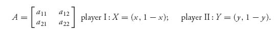
For any mixed strategies, we have E(X, Y) = X AYT, which, written out, is
![]()
Now here is the theorem giving the solution of this game.
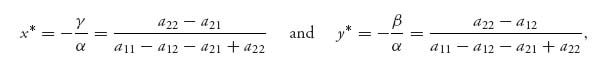
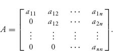
Theorem 2.1.1 In the 2 × 2 game with matrix A, assume that there are no pure optimal strategies. If we set
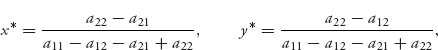
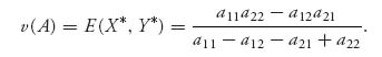
then X* =(x*, 1 − x*), Y* =(y*, 1 − y*) are optimal mixed strategies for players I and II, respectively. The value of the game is
Remarks
where
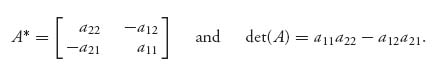
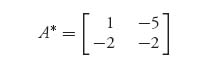
Recall that the inverse of a 2 × 2 matrix is found by swapping the main diagonal numbers, and putting a minus sign in front of the other diagonal numbers, and finally dividing by the determinant of the matrix. A* is exactly the first two steps, but we don’t divide by the determinant. The matrix we get is defined even if the matrix A doesn’t have an inverse. Remember, however, that we need to make sure that the matrix doesn’t have optimal pure strategies first.
Note, too, that if det (A) = 0, the value of the game is zero.
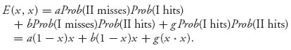
Here is why the formulas hold. Write f(x, y) = E(X, Y), where X =(x, 1 − x), Y = (y, 1 − y), and 0 ≤ x, y ≤ 1. Then
(2.1)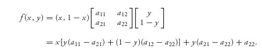
By assumption there are no optimal pure strategies, and so the extreme points of f will be found inside the intervals 0 < x, y < 1. But that means that we may take the partial derivatives of f with respect to x and y and set them equal to zero to find all the possible critical points. The function f has to look like the function depicted in Figure 2.1.
FIGURE 2.1 Concave in x, convex in y, saddle at ![]()
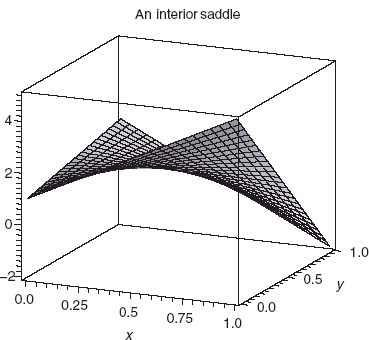
Figure 2.1 is the graph of f(x, y) = X AYT taking ![]() It is a concave–convex function that has a saddle point at x =
It is a concave–convex function that has a saddle point at x = ![]() , y =
, y = ![]() . You can see now why it is called a saddle.
. You can see now why it is called a saddle.
Returning to our general function f(x, y) in (2.1), take the partial derivatives and set to zero:
where we have set
![]()
Note that if α = 0, the partials are never zero (assuming β, γ ≠ 0), and that would imply that there are pure optimal strategies (in other words, the min and max must be on the boundary). The existence of a pure saddle is ruled out by assumption. We solve where the partial derivatives are zero to get
which is the same as what the theorem says. How do we know this is a saddle and not a min or max of f? The reason is because if we take the second derivatives, we get the matrix of second partials (called the Hessian):
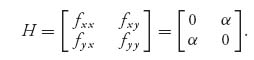
Since det (H) = − α2 < (unless α = 0, which is ruled out) a theorem in elementary calculus says that an interior critical point with this condition must be a saddle.1
So the procedure is as follows. Look for pure strategy solutions first (calculate v− and v+ and see if they’re equal), but if there aren’t any, use the formulas to find the mixed strategy solutions.
Remark One final comment about 2 × 2 games is that if there is no pure saddle, then by Theorem 1.3.8 we know that E(X*, 1) = v = E(X*, 2) and E(1, Y*) = v = E(2, Y*), when (X*, Y*) is a saddle point. Solving these equations results in exactly the same formulas as using calculus.
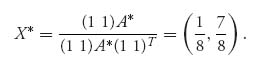
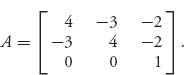
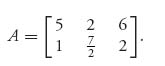
Example 2.1 In the game with 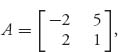 we see that v− = 1 < v+=2, so there is no pure saddle for the game. If we apply the formulas, we get the mixed strategies X* =(
![]() ,
, ![]() ) and Y* = (
) and Y* = (![]() ,
, ![]() ) and the value of the game is v(A) =
) and the value of the game is v(A) = ![]() . Note here that
. Note here that
and det (A) = − . The matrix formula for player I gives
Problems
2.1 In a simplified analysis of a football game, suppose that the offense can only choose a pass or run, and the defense can choose only to defend a pass or run. Here is the matrix in which the payoffs are the average yards gained:
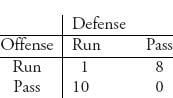
The offense’s goal is to maximize the average yards gained per play. Find v(A) and the optimal strategies using the explicit formulas. Check your answers by solving graphically as well.
2.2 Suppose that an offensive pass against a run defense now gives 12 yards per play on average to the offense (so the 10 in the previous matrix changes to a 12). Believe it or not, the offense should pass less, not more. Verify that and give a game theory (not math) explanation of why this is so.
2.3 Does the same phenomenon occur for the defense? To answer this, compare the original game in Problem 2.1 to the new game in which the defense reduces the number of yards per run to 6 instead of 8 when defending against the pass. What happens to the optimal strategies?
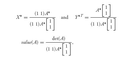
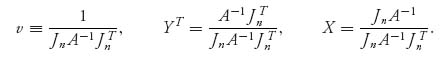
2.4 If the matrix of the game has an inverse, the formulas can be simplified to
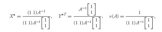
where 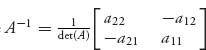 . This requires that det (A) ≠ 0. Construct an example to show that even if A−1 does not exist, the original formulas with A−1 replaced by A* still hold but now v(A) = 0.
2.5 Show that the formulas in the theorem are exactly what you would get if you solved the 2 × 2 game graphically (i.e., using Theorem 1.3.8) under the assumption that no pure saddle point exists.
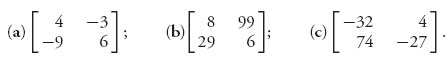
2.6 Solve the 2 × 2 games using the formulas and check by solving graphically:
2.7 Give an example to show that when optimal pure strategies exist, the formulas in the theorem won’t work.
2.8 Let A = (aij), i, j = 1, 2. Show that if a11+ a22 = a12+a22, then v+ = v− or, equivalently, there are optimal pure strategies for both players. This means that if you end up with a zero denominator in the formula for v(A), it turns out that there had to be a saddle in pure strategies for the game and hence the formulas don’t apply from the outset.
2.2 Invertible Matrix Games
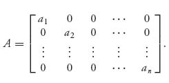
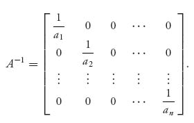
In this section, we will solve the class of games in which the matrix A is square, say, n × n and invertible, so det (A) ≠ 0 and A−1 exists and satisfies A−1A = AA−1 = In × n. The matrix In × n is the n × n identity matrix consisting of all zeros except for ones along the diagonal. For the present let us suppose that
Player I has an optimal strategy that is completely mixed, specifically, X = (x1, ..., xn), and xi > 0, i = 1, 2, ..., n. So player I plays every row with positive probability.
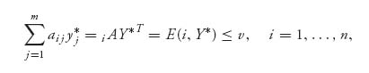
By the Properties of Strategies (Section 1.3.1) (see also Theorem 1.3.8) we know that this implies that every optimal Y strategy for player II, must satisfy
![]()
Y played against any row will give the value of the game. If we write Jn = (1 1 ... 1) for the row vector consisting of all 1s, we can write
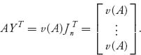
Now, if v(A) = 0, then AYT = 0 JnT = 0, and this is a system of n equations in the n unknowns Y = (y1, ..., yn). It is a homogeneous linear system. Since A is invertible, this would have the one and only solution YT = A−1 0 = 0. But that is impossible if Y is a strategy (the components must add to 1). So, if this is going to work, the value of the game cannot be zero, and we get, by multiplying both sides of (1) by A−1, the following equation:
![]()
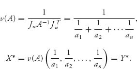
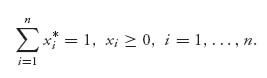
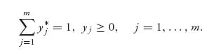
This gives us Y if we knew v(A). How do we get that? The extra piece of information we have is that the components of Y add to 1 ![]() . So
. So
![]()
and therefore,
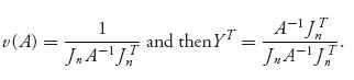
We have found the only candidate for the optimal strategy for player II assuming that every component of X is greater than 0. However, if it turns out that this formula for Y has at least one yj < 0, something would have to be wrong; specifically, it would not be true that X was completely mixed because that was our hypothesis. But, if it turns out that yj ≥ 0 for every component, we could try to find an optimal X for player I by the exact same method. This would give us
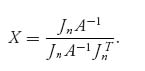
This method will work if the formulas we get for X and Y end up satisfying the condition that they are strategies. If either X or Y has a negative component, then it fails. But notice that the strategies do not have to be completely mixed as we assumed from the beginning, only bona fide strategies.
Here is a summary of what we know.
Theorem 2.2.1 Assume that
1. An × n has an inverse A−1.
2. ![]()
3. v(A) ≠ 0.
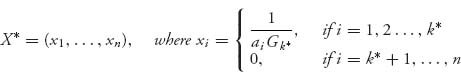
Set X = m (x1, ..., xn), Y =(y1, ..., ym), and
If xi ≥ 0, i = 1, ..., n and yj ≥ 0, j = 1, ..., n, we have that v = v(A) is the value of the game with matrix A and (X, Y) is a saddle point in mixed strategies.
Now the point is that when we have an invertible game matrix, we can always use the formulas in the theorem to calculate the number v and the vectors X and Y. If the result gives vectors with nonnegative components, then, by the properties (Section 1.3.1) of games, v must be the value, and (X, Y) is a saddle point. Note that, directly from the formulas, Jn YT = 1 and X JnT = 1, so the components given in the formulas will automatically sum to 1; it is only the sign of the components that must be checked.
Here is a simple direct verification that (X, Y) is a saddle and v is the value assuming xi ≥ 0, yj ≥ 0. Let Y’ ![]() Sn be any mixed strategy and let X be given by the formula
Sn be any mixed strategy and let X be given by the formula ![]() Then, since
Then, since ![]() we have
we have
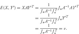
Similarly, for any X′ ![]() Sn, E(X ′, Y) = v, and so (X, Y) is a saddle and v is the value of the game by the Theorem 1.3.8 or Property 1 of (Section 1.3.1).
Sn, E(X ′, Y) = v, and so (X, Y) is a saddle and v is the value of the game by the Theorem 1.3.8 or Property 1 of (Section 1.3.1).
Incidentally, these formulas match the formulas when we have a 2 × 2 game with an invertible matrix because then A−1 = (1/det (A))A*.
Remark In order to guarantee that the value of a game is not zero, we may add a constant to every element of A that is large enough to make all the numbers of the matrix positive. In this case, the value of the new game could not be zero. Since v(A + b) = v(A) + b, where b is the constant added to every element, we can find the original v(A) by subtracting b. Adding the constant to all the elements of A will not change the probabilities of using any particular row or column; that is, the optimal mixed strategies are not affected by doing that.
Even if our original matrix A does not have an inverse, if we add a constant to all the elements of A, we get a new matrix A + b and the new matrix may have an inverse (of course, it may not as well). We may have to try different values of b. Here is an example.
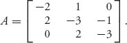
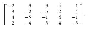
Example 2.2 Consider the matrix
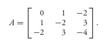
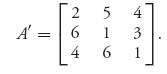
This matrix has negative and positive entries, so it’s possible that the value of the game is zero. The matrix does not have an inverse because the determinant of A is 0. So, let’s try to add a constant to all the entries to see if we can make the new matrix invertible. Since the largest negative entry is −4, let’s add 5 to everything to get
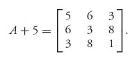
This matrix does have an inverse given by
Next, we calculate using the formulas ![]() and
and
Since both X and Y are strategies (they have nonnegative components), the theorem tells us that they are optimal and the value of our original game is v(A) = v − 5 = 0.
The next example shows what can go wrong.
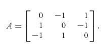
Example 2.3 Let
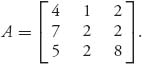
Then it is immediate that v− = v+ = 2 and there is a pure saddle X* = (0, 0, 1), Y* =(0, 1, 0). If we try to use Theorem 2.2.1, we have det (A) = 10, so A−1 exists and is given by
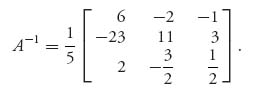
If we use the formulas of the theorem, we get
and
Obviously these are completely messed up (i.e., wrong). The problem is that the components of X and Y are not nonnegative even though they do sum to 1.
Remark What can we do if the matrix is not square? Obviously we can’t talk about inverses of nonsquare matrices. However, we do have the following theorem that reduces the problem to a set of square matrices. This theorem is mostly of theoretical interest because for large matrices it’s not feasible to implement it.
Theorem 2.2.2 Let An × m be a matrix game.
2.2.1 COMPLETELY MIXED GAMES
We just dealt with the case that the game matrix is invertible, or can be made invertible by adding a constant. A related class of games that are also easy to solve is the class of completely mixed games. We have already mentioned these earlier, but here is a precise definition.
Definition 2.2.3 A game is completely mixed if every saddle point consisting of strategies X =(x1, ..., xn) ![]() Sn, Y = (y1, ..., ym)
Sn, Y = (y1, ..., ym) ![]() Sm satisfies the property xi > 0, i = 1, 2, ..., n and yj > 0, j = 1, 2, ..., m. Every row and every column is used with positive probability.
Sm satisfies the property xi > 0, i = 1, 2, ..., n and yj > 0, j = 1, 2, ..., m. Every row and every column is used with positive probability.
If you know, or have reason to believe, that the game is completely mixed ahead of time, then there is only one saddle point! It can also be shown that for completely mixed games with a square game matrix if you know that v(A) ≠ 0, then the game matrix A must have an inverse, A−1. In this case the formulas for the value and the saddle

from Theorem 2.2.1 will give the completely mixed saddle. The procedure is that if you are faced with a game and you think that it is completely mixed, then solve it using the formulas and verify.
Example 2.4 Hide and Seek. Suppose that we have a1 > a2 > ![]() > an > 0. The game matrix is
> an > 0. The game matrix is
Because ai > 0 for every i = 1, 2, ..., n, we know det (A) = a1a2![]() an>0, so A−1 exists. It seems pretty clear that a mixed strategy for both players should use each row or column with positive probability; that is, we think that the game is completely mixed. In addition, since v− = 0 and v+ = an, the value of the game satisfies 0 ≤ v(A) ≤ an. Choosing X =(
an>0, so A−1 exists. It seems pretty clear that a mixed strategy for both players should use each row or column with positive probability; that is, we think that the game is completely mixed. In addition, since v− = 0 and v+ = an, the value of the game satisfies 0 ≤ v(A) ≤ an. Choosing X =(![]() , ...,
, ..., ![]() ) we see that
) we see that
so that v(A) = maxX minY X AYT > 0. This isn’t a fair game for player II. It is also easy to see that
Then, we may calculate from Theorem 2.2.1 that
The strategies X*, Y* are legitimate strategies and they are optimal. Notice that for any i = 1, 2, ..., n, we obtain
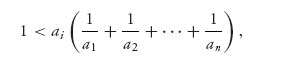
so that v(A)< min (a1, a2, ..., an) = an.
Our last example again shows how the invertible matrix theorem can be used, but with caution.
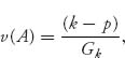
Example 2.5 This is an example on optimal target choice and defense. Suppose a company, player I, is seeking to takeover one of n companies that have values to player I a1 > a2>![]() > an>0. These companies are managed by a private equity firm that can defend exactly one of the companies from takeover. Suppose that an attack made on company n has probability 1 − p of being taken over if it is defended. Player I can attack exactly one of the companies and player II can choose to defend exactly one of the n small companies. If an attack is made on an undefended company, the payoff to I is ai. If an attack is made on a defended company, I’s payoff is (1 − p)ai.
> an>0. These companies are managed by a private equity firm that can defend exactly one of the companies from takeover. Suppose that an attack made on company n has probability 1 − p of being taken over if it is defended. Player I can attack exactly one of the companies and player II can choose to defend exactly one of the n small companies. If an attack is made on an undefended company, the payoff to I is ai. If an attack is made on a defended company, I’s payoff is (1 − p)ai.
The payoff matrix is
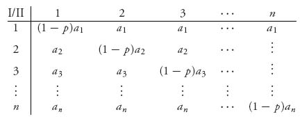
Let’s start with n = 3. We want to find the value and optimal strategies.
Since ![]() the invertible matrix theorem can be used if
the invertible matrix theorem can be used if ![]() and the resulting strategies are legit. We have
and the resulting strategies are legit. We have
and X* = v(A)J3 A−1, resulting in
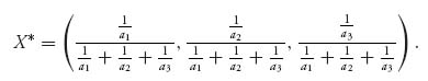
The formula for ![]() gives
gives
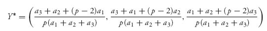
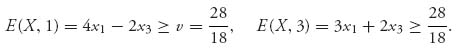
Since p −2 < 0, Y* may not be a legitimate strategy for player II. Nevertheless, player I’s strategy is legitimate and is easily verified to be optimal by showing that E(X*, j) ≥ v(A), j = 1, 2, 3.
For example if we take p = 0.1, ai = 4 − i, i = 1, 2, 3, we calculate from the formulas above,
![]()
which is obviously not a strategy for player II. The invertible theorem gives us the right thing for v and X* but not for Y*. Another approach is needed.
The idea is still to use part of the invertible theorem for v(A) and X* but then to do a direct derivation of Y*. We will follow an argument due to Dresher (1981).2
Because of the structure of the payoffs it seems reasonable that an optimal strategy for player II (and I as well) will be of the form Y = (y1, ..., yk, 0, 0, 0), that is, II will not use the columns k + 1, ..., n, for some k > 1. We need to find the nonzero yj′s and the value of k.
We have the optimal strategy X* for player I and we know that x1 > 0, x2 > 0. By Theorem 1.3.8 and Proposition 1.3.10, we then know that E (1, Y*) = v, E(2, Y*) = v. Written out, this is
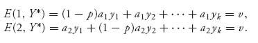
Using the fact that ![]() we have
we have
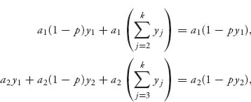
and a2 (1 − py2) = a1(1 − py1). Solving for y2 we get
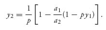
In general, the same argument using the fact that x1 > 0 and xi > 0, i = 2, 3, ..., k results in all the ![]() in terms of y1:
in terms of y1:
The index k > 1 is yet to be determined and remember we are setting yj = 0, j = k + 1, ..., n. Again using the fact that ![]() we obtain after some algebra the formula
we obtain after some algebra the formula
Here, ![]()
Now note that if we use the results from the invertible matrix theorem for v and X*, we may define
and
and X* is still a legitimate strategy for player I and v(A) will still be the value of the game for any value of k ≤ n. You can easily verify that E(X*, j) = v(A) for each column j. Now we have the candidates in hand we may verify that they do indeed solve the game.
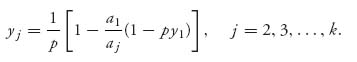
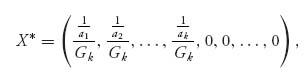
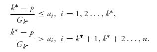
Theorem 2.2.4 Set ![]() Notice that Gk + 1 ≥ Gk. Let k* be the value of i giving
Notice that Gk + 1 ≥ Gk. Let k* be the value of i giving ![]() Then,
Then,
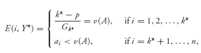
is optimal for player I, and Y* = (y1, y2, ..., yn),
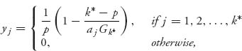
is optimal for player II. In addition, ![]() is the value of the game.
is the value of the game.
Proof. The only thing we need to verify is that Y* is a legitimate strategy for player II and is optimal for that player.
First, let’s consider the function f(k) = k − akGk. We have
![]()
Since ak > ak + 1,
![]()
We conclude that f(k + 1) > f(k), that is, f is a strictly increasing function of k = 1, 2... . Also f(1) = 1 − a1G1 = 0 and we may set f(n + 1) = any big positive integer. We can then find exactly one index k* so that f(k*) ≤ p < f(k* + 1) and this will be the k* in the statement of the theorem. We will show later that it is characterized as stated in the theorem.
Now for this k*, we have
![]()
Since the ![]() decrease, we get
decrease, we get
Since
this proves by Theorem 1.3.8 that Y* is optimal for player II. Notice also that yj ≥ 0 for all j = 1, 2, ..., n since by definition
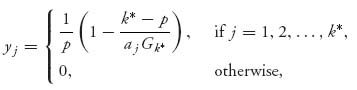
and we have shown that
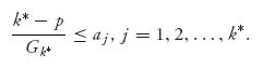
Hence, Y* is a legitimate strategy.
Finally, we show that k* can also be characterized as follows: k* is the value of i achieving ![]() To see why, the function
To see why, the function ![]() has a maximum value at some value k =
has a maximum value at some value k = ![]() . That means
. That means ![]() and
and ![]() Using the definition of
Using the definition of ![]() , we get
, we get
![]()
which is what k* must satisfy. Consequently, ![]() = k* and we are done.
= k* and we are done. ![]()
In the problems you will calculate X*, Y*, and v for specific values of p, ai.
Problems
2.9 Consider Example 2.5 and let p = 0.5, a1 = 9, a2 = 7, a3 = 6, a4 = 1. Find v(A), X*, Y*, solving the game. Find the value of k* first.
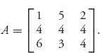
2.10 Consider the matrix game
Show that there is a saddle in pure strategies at (1, 3) and find the value. Verify that X* = (![]() , 0,
, 0, ![]() ), Y* = (
), Y* = (![]() , 0,
, 0, ![]() ) is also an optimal saddle point. Does A have an inverse? Find it and use the formulas in the theorem to find the optimal strategies and value.
) is also an optimal saddle point. Does A have an inverse? Find it and use the formulas in the theorem to find the optimal strategies and value.
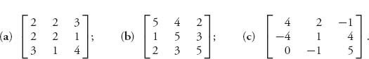
2.11 Solve the following games:
2.12 To underscore that the formulas can be used only if you end up with legitimate strategies, consider the game with matrix
2.13 Show that value (A + b) = value(A) + b for any constant b, where by A + b = (aij + b) is meant A plus the matrix with all entries = b. Show also that (X, Y) is a saddle for the matrix A + b if and only if it is a saddle for A.
2.14 Derive the formula for ![]() assuming the game matrix has an inverse. Follow the same procedure as that in obtaining the formula for Y.
assuming the game matrix has an inverse. Follow the same procedure as that in obtaining the formula for Y.
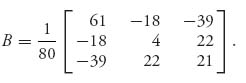
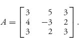
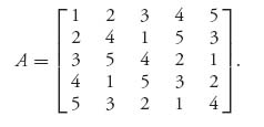
2.15 A magic square game has a matrix in which each row has a row sum that is the same as each of the column sums. For instance, consider the matrix
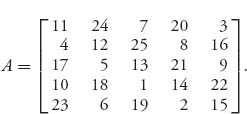
This is a magic square of order 5 and sum 65. Find the value and optimal strategies of this game and show how to solve any magic square game.
2.16 Why is the hide-and-seek game in Example 2.4 called that? Determine what happens in the hide-and-seek game if there is at least one ak = 0.
2.17 Solve the hide-and-seek game in Example 2.4 with matrix ![]() 1, 2, ..., n, and aij = 0, i ≠ j. Find the general solution and give the exact solution when n = 5.
1, 2, ..., n, and aij = 0, i ≠ j. Find the general solution and give the exact solution when n = 5.
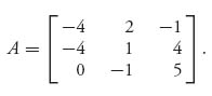
2.18 For the game with matrix
we determine that the optimal strategy for player II is ![]() We are also told that player I has an optimal strategy X which is completely mixed. Given that the value of the game is
We are also told that player I has an optimal strategy X which is completely mixed. Given that the value of the game is ![]() , find X.
, find X.
2.19 A triangular game is of the form
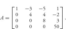
Solve the game by finding v(A) and the optimal strategies.
2.20 Another method that can be used to solve a game uses calculus to find the interior saddle points. For example, consider
A strategy for each player is of the form X =(x1, x2, 1 − x1 − x2), Y = (y1, y2, 1 − y1 − y2), so we consider the function f(x1, x2, y1, y2) = XAYT. Now solve the system of equations
![]()
to get X* and Y*. If these are legitimate completely mixed strategies, then you can verify that they are optimal and then find v(A). Carry out these calculations for A and verify that they give optimal strategies.
2.21 Consider the Cat versus Rat game (Example 1.3). The game matrix is 16 × 16 and consists of 1s and 0s, but the matrix can be considerably reduced by eliminating dominated rows and columns. The game reduces to the 3 × 3 game
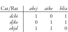
Now solve the game.
2.22 In tennis, two players can choose to hit a ball left, center, or right of where the opposing player is standing. Name the two players I and II and suppose that I hits the ball, while II anticipates where the ball will be hit. Suppose that II can return a ball hit right 90% of the time, a ball hit left 60% of the time, and a ball hit center 70% of the time. If II anticipates incorrectly, she can return the ball only 20% of the time. Score a return as + 1 and a ball not returned as − 1. Find the game matrix and the optimal strategies.
2.3 Symmetric Games
Symmetric games are important classes of two-person games in which the players can use the exact same set of strategies and any payoff that player I can obtain using strategy X can be obtained by player II using the same strategy Y = X. The two players can switch roles. Such games can be quickly identified by the rule that A = − AT. Any matrix satisfying this is said to be skew symmetric. If we want the roles of the players to be symmetric, then we need the matrix to be skew symmetric.
Why is skew symmetry the correct thing? Well, if A is the payoff matrix to player I, then the entries represent the payoffs to player I and the negative of the entries, or − A represent the payoffs to player II. So player II wants to maximize the column entries in − A. This means that from player II’s perspective, the game matrix must be (− A)T because it is always the row player by convention who is the maximizer; that is, A is the payoff matrix to player I and − AT is the payoff to player II. If we want the payoffs to player II to be the same as the payoffs to player I, then we must have the same game matrices for each player and so A = − AT. If this is the case, the matrix must be square, aij = − aji, and the diagonal elements of A, namely, aii, must be 0. We can say more. In what follows it is helpful to keep in mind that for any appropriate size matrices ABT = BT AT.
Theorem 2.3.1 For any skew symmetric game v(A) = 0 and if X* is optimal for player I, then it is also optimal for player II.
Proof. First, let X be any strategy for I. Then
![]()
Therefore, E(X, X) = 0 and any strategy played against itself has zero payoff.
Next for any strategies (X, Y), we have
(2.3)![]()
Now let (X*, Y*) be a saddle point for the game so that
![]()
Hence, from the saddle point definition and (2. 3), we obtain
![]()
This says
![]()
But this says that Y* is optimal for player I and X* is optimal for player II and also that E(X*, Y*) = − E(Y*, X*) ![]() v(A) = 0.
v(A) = 0.
Finally, we show that (X*, X*) is also a saddle point. We already know from the first step that E(X*, X*) = 0, so we need to show
![]()
Since E(X*, X*) = E(X*, Y*) = 0 ≤ E(X*, Y) for all Y, the second part of the inequality is true. Since E(X*, X*) = E(Y*, X*) ≥ E(X, X*) for all X, the first part of the inequality is true, and we are done. ![]()
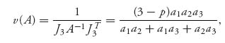
Example 2.6 How to solve 3 × 3 Symmetric Games. For any 3 × 3 symmetric game, we must have
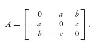
You can check that this matrix has a zero determinant so there is no inverse. Also, the value of a symmetric game is zero. We could try to add a constant to everything, get a nonzero value and then see if we can invert the matrix to use the invertible game theorem. Instead, we try a direct approach that will always work for symmetric games.
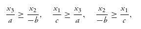
Naturally, we have to rule out games with a pure saddle. Any of the following conditions gives a pure saddle point:
Here’s why. Let’s assume that a ≤ 0, c ≥ 0. In this case if b ≤ 0 we get v− =max{min{a, b}, 0, −c} = 0 and v+ = min{max{− a, − b}, 0, c} = 0, so there is a saddle in pure strategies at (2, 2). All cases are treated similarly. To have a mixed strategy, all three of these must fail.
We next solve the case a > 0, b < 0, c > 0 so there is no pure saddle and we look for the mixed strategies. The other cases are similar and it is the approach you need to know.
Let player I’s optimal strategy be X* = (x1, x2, x3). Then
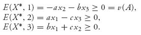
Each one is nonnegative since E(X*, Y)≥ 0 = v(A), for all Y. Now, since a > 0, b < 0, i c > 0, we get
so
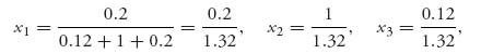
and we must have equality throughout. It is then true that ![]() Since they must sum to one, x1+x2+x3 = 1 and we can find the optimal strategies after a little algebra as
Since they must sum to one, x1+x2+x3 = 1 and we can find the optimal strategies after a little algebra as ![]() where
where ![]() . The value of the game, of course, is zero.
. The value of the game, of course, is zero.
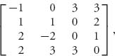
For example, the matrix
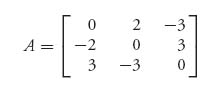
is skew symmetric and does not have a saddle point in pure strategies as you can easily check. We know that v(A) = 0 and if X =(x1, x2, x3) is optimal for player I, then E(X, j) ≥ 0, j = 1, 2, 3. This gives us
![]()
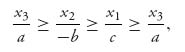
which implies
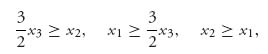
or x2 ≥ x1 ≥ ![]() x3 ≥ x2, and we have equality throughout. Since x1+x2+x3 = 1, we may calculate x1 =
x3 ≥ x2, and we have equality throughout. Since x1+x2+x3 = 1, we may calculate x1 = ![]() = x2, x3 =
= x2, x3 = ![]() . Since the game is symmetric we have shown v = 0, X* = Y* = (
. Since the game is symmetric we have shown v = 0, X* = Y* = (![]() ,
, ![]() ,
, ![]() ).
).
Example 2.7 A ubiquitous game is rock-paper-scissors. Each player chooses one of rock, paper or scissors. The rules are Rock beats Scissors; Scissors beats Paper; Paper beats Rock. We’ll use the following payoff matrix:
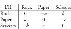
Assume that a, b, c > 0. Then v−= max {−a, −c, −b} < 0 and v+= min{a, c, b} > 0 so this game does not have a pure saddle point. Since the matrix is skew symmetric we know that v(A) = 0 and X* = Y* is a saddle point, so we need only find X* = (x1, x2, x3). We have
![]()
Therefore, we have equality throughout, and

In the standard game, a = b = c = 1 and the optimal strategy for each player is X* = (![]() ,
, ![]() ,
, ![]() ), which is what you would expect when the payoffs are all the same. But if the payoffs are not the same, say a = 1, b= 2, c = 3 then the optimal strategy for each player is
), which is what you would expect when the payoffs are all the same. But if the payoffs are not the same, say a = 1, b= 2, c = 3 then the optimal strategy for each player is ![]()
Example 2.8 Alexander Hamilton was challenged to a duel with pistols by Aaron Burr after Hamilton wrote a defamatory article about Burr in New York. We will analyze one version of such a duel by the two players as a game with the object of trying to find the optimal point at which to shoot. First, here are the rules.
Each pistol has exactly one bullet. They will face each other starting at 10 paces apart and walk toward each other, each deciding when to shoot. In a silent duel, a player does not know whether the opponent has taken the shot. In a noisy duel, the players know when a shot is taken. This is important because if a player shoots and misses, he is certain to be shot by the person he missed. The Hamilton–Burr duel will be considered as a silent duel because it is more interesting. We leave as an exercise the problem of the noisy duel.
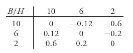
We assume that each player’s accuracy will increase the closer the players are. In a simplified version, suppose that they can choose to fire at 10 paces, 6 paces, or 2 paces. Suppose also that the probability that a shot hits and kills the opponent is 0.2 at 10 paces, 0.4 at 6 paces, and 1.0 at 2 paces. An opponent who is hit is assumed killed.
If we look at this as a zero sum two-person game, the player strategies consist of the pace distance at which to take the shot. The row player is Burr (B), and the column player is Hamilton (H). Incidentally, it is worth pointing out that the game analysis should be done before the duel is actually carried out.
We assume that the payoff to both players is + 1 if they kill their opponent, − 1 if they are killed, and 0 if they both survive.
So here is the matrix setup for this game.
To see where these numbers come from, let’s consider the pure strategy (6, 10), so Burr waits until 6 to shoot (assuming that he survived the shot by Hamilton at 10) and Hamilton chooses to shoot at 10 paces. Then the expected payoff to Burr is
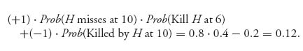
The rest of the entries are derived in the same way.
This is a symmetric game with skew symmetric matrix so the value is zero and the optimal strategies are the same for both Burr and Hamilton, as we would expect since they have the same accuracy functions. In this example, there is a pure saddle at position (3, 3) in the matrix, so that X* = (0, 0, 1) and Y* = (0, 0, 1). Both players should wait until the probability of a kill is certain.
To make this game a little more interesting, suppose that the players will be penalized if they wait until 2 paces to shoot. In this case, we may use the matrix
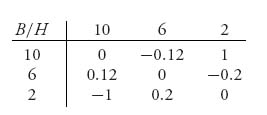
This is still a symmetric game with skew symmetric matrix, so the value is still zero and the optimal strategies are the same for both Burr and Hamilton. To find the optimal strategy for Burr, we can remember the formulas or, even better, the procedure. So here is what we get knowing that E(X*, j) ≥ 0, j = 1, 2, 3:
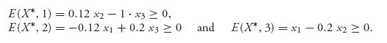
These give us
![]()
which means equality all the way. Consequently,
or x1 = 0.15, x2 = 0.76, x3 = 0.09, so each player will shoot, with probability 0.76 at 6 paces.
In the real duel, that took place on July 11, 1804, Alexander Hamilton, who was the first US Secretary of the Treasury and widely considered to be a future president and a genius, was shot by Aaron Burr, who was Thomas Jefferson’s vice president of the United States and who also wanted to be president. In fact, Hamilton took the first shot, shattering the branch above Burr’s head. Witnesses report that Burr took his shot some 3 or 4 seconds after Hamilton. Whether or not Hamilton deliberately missed his shot is disputed to this day. Nevertheless, Burr’s shot hit Hamilton in the torso and lodged in his spine, paralyzing him. Hamilton died of his wounds the next day. Aaron Burr was charged with murder but was later either acquitted or the charge was dropped (dueling was in the process of being outlawed). The duel was the end of the ambitious Burr’s political career, and he died an ignominious death in exile. Interestingly, both Burr and Hamilton had been involved in numerous duels in the past. In a tragic historical twist, Alexander Hamilton’s son, Phillip, was earlier killed in a duel on November 23, 1801.
Problems
2.23 Find the matrix for a noisy Hamilton–Burr duel and solve the game.
2.24 Each player displays either one or two fingers and simultaneously guesses how many fingers the opposing player will show. If both players guess correctly or both incorrectly, the game is a draw. If only one guesses correctly, that player wins an amount equal to the total number of fingers shown by both players. Each pure strategy has two components: the number of fingers to show and the number of fingers to guess. Find the game matrix and the optimal strategies.
2.25 This exercise shows that symmetric games are more general than they seem at first and in fact this is the main reason they are important. Assuming that An × m is any payoff matrix with value (A)> 0, define the matrix B that will be of size (n+m+1) × (n+m+1), by
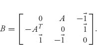
The notation ![]() , for example, in the third row and first column, is the 1 × n matrix consisting of all 1s. B is a skew symmetric matrix and it can be shown that if P = (p1, ..., pn, q1, ..., qm, γ) is an optimal strategy for matrix B, then, setting
, for example, in the third row and first column, is the 1 × n matrix consisting of all 1s. B is a skew symmetric matrix and it can be shown that if P = (p1, ..., pn, q1, ..., qm, γ) is an optimal strategy for matrix B, then, setting
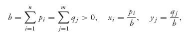
we have X = (x1, ..., xn), Y =(y1, ..., ym) as a saddle point for the game with matrix A. In addition, value(A) = ![]() The converse is also true. Verify all these points with the matrix
The converse is also true. Verify all these points with the matrix
2.4 Matrix Games and Linear Programming
Linear programming is an area of optimization theory developed since World War II that is used to find the minimum (or maximum) of a linear function of many variables subject to a collection of linear constraints on the variables. It is extremely important to any modern economy to be able to solve such problems that are used to model many fundamental problems that a company may encounter. For example, the best routing of oil tankers from all of the various terminals around the world to the unloading points is a linear programming problem in which the oil company wants to minimize the total cost of transportation subject to the consumption constraints at each unloading point. But there are millions of applications of linear programming, which can range from the problems just mentioned to modeling the entire US economy. One can imagine the importance of having a very efficient way to find the optimal variables involved. Fortunately, George Dantzig, 3 in the 1940s, because of the necessities of the war effort, developed such an algorithm, called the simplex method that will quickly solve very large problems formulated as linear programs.
Mathematicians and economists working on game theory (including von Neumann), once they became aware of the simplex algorithm, recognized the connection.4 After all, a game consists in minimizing and maximizing linear functions with linear things all over the place. So a method was developed to formulate a matrix game as a linear program (actually two of them) so that the simplex algorithm could be applied.
This means that using linear programming, we can find the value and optimal strategies for a matrix game of any size without any special theorems or techniques. In many respects, this approach makes it unnecessary to know any other computational approach. The downside is that in general one needs a computer capable of running the simplex algorithm to solve a game by the method of linear programming. We will show how to set up the game in two different ways to make it amenable to the linear programming method and also the Maple and Mathematica commands to solve the problem. We show both ways to set up a game as a linear program because one method is easier to do by hand (the first) since it is in standard form. The second method is easier to do using Maple and involves no conceptual transformations. Let’s get on with it.
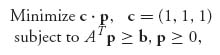
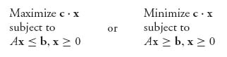
A linear programming problem is a problem of the standard form (called the primal program):
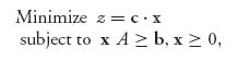
where c = (c1, ..., cn), x = (x1, ..., xn), An × m; is an n × m matrix, and b = (b1, ..., bm).
The primal problem seeks to minimize a linear objective function, z(x)= c ![]() x, over a set of constraints (namely, x
x, over a set of constraints (namely, x ![]() A ≥ b) that are also linear. You can visualize what happens if you try to minimize or maximize a linear function of one variable over a closed interval on the real line. The minimum and maximum must occur at an endpoint. In more than one dimension, this idea says that the minimum and maximum of a linear function over a variable that is in a convex set must occur on the boundary of the convex set. If the set is created by linear inequalities, even more can be said, namely, that the minimum or maximum must occur at an extreme point, or corner point, of the constraint set. The method for solving a linear program is to efficiently go through the extreme points to find the best one. That is essentially the simplex method.
A ≥ b) that are also linear. You can visualize what happens if you try to minimize or maximize a linear function of one variable over a closed interval on the real line. The minimum and maximum must occur at an endpoint. In more than one dimension, this idea says that the minimum and maximum of a linear function over a variable that is in a convex set must occur on the boundary of the convex set. If the set is created by linear inequalities, even more can be said, namely, that the minimum or maximum must occur at an extreme point, or corner point, of the constraint set. The method for solving a linear program is to efficiently go through the extreme points to find the best one. That is essentially the simplex method.
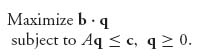
For any primal there is a related linear program called the dual program:
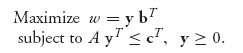
A very important result of linear programming, which is called the duality theorem, states that if we solve the primal problem and obtain the optimal objective z = z*, and solve the dual obtaining the optimal w = w*, then z* = w*. In our game theory formulation to be given next, this theorem will tell us that the two objectives in the primal and the dual will give us the value of the game.
We will now show how to formulate any matrix game as a linear program. We need the primal and the dual to find the optimal strategies for each player.
2.4.1 SETTING UP THE LINEAR PROGRAM: METHOD 1
Let A be the game matrix. We may assume aij> 0 by adding a large enough constant to A if that isn’t true. As we have seen earlier, adding a constant won’t change the strategies and will only add a constant to the value of the game.
Hence we assume that v(A) > 0. Now consider the properties of optimal strategies from Section 1.3.1. Player I looks for a mixed strategy X =(x1, ..., xn) so that
(2.4)![]()
where ![]() and v > 0 is as large as possible, because that is player I’s reward. It is player I’s objective to get the largest value possible. Note that we don’t have any connection with player II here except through the inequalities that come from player II using each column.
and v > 0 is as large as possible, because that is player I’s reward. It is player I’s objective to get the largest value possible. Note that we don’t have any connection with player II here except through the inequalities that come from player II using each column.
We will make this problem look like a regulation linear program. We change variables by setting
![]()
This is where we need v > 0. Then ![]() implies that
implies that
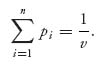
Thus, maximizing v is the same as minimizing ![]() This gives us our objective, namely, to minimize
This gives us our objective, namely, to minimize ![]() In matrix form, this is the same as
In matrix form, this is the same as ![]() where p=(p1, ..., pn) and Jn = (1, 1, ..., 1).
where p=(p1, ..., pn) and Jn = (1, 1, ..., 1).
For the constraints, if we divide the inequalities (2. 4) by v and switch to the new variables, we get the set of constraints
![]()
Now we summarize this as a linear program.
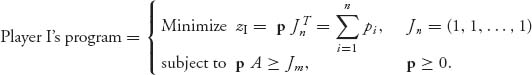
Note that the constraint of the game ![]() is used to get the objective function! It is not one of the constraints of the linear program. The set of constraints is
is used to get the objective function! It is not one of the constraints of the linear program. The set of constraints is
![]()
Also p ≥ 0 means pi ≥ 0, i = 1, ..., n.
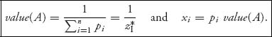
Once we solve player I’s program, we will have in our hands the optimal p = (p1, ..., pn) that minimizes the objective ![]() The solution will also give us the minimum objective zI, labeled zI*.
The solution will also give us the minimum objective zI, labeled zI*.
Unwinding the formulation back to our original variables, we find the optimal strategy X for player I and the value of the game as follows:
Remember, too, that if you had to add a constant to the matrix to ensure v(A) > 0, then you have to subtract that same constant to get the value of the original game.
Now we look at the problem for player II. Player II wants to find a mixed strategy ![]() so that
so that
![]()
with u > 0 as small as possible. Setting
![]()
we can restate player II’s problem as the standard linear programming problem.
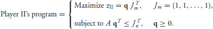
Player II’s problem is the dual of player I’s. At the conclusion of solving this program, we are left with the optimal maximizing vector q = (q1, ..., qm) and the optimal objective value zII*. We obtain the optimal mixed strategy for player II and the value of the game from
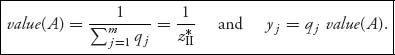
However, how do we know that the value of the game using player I’s program will be the same as that given by player II’s program? The important duality theorem mentioned above and given explicitly below tells us that is exactly true, and so ![]()
Remember again that if you had to add a number to the matrix to guarantee that v > 0, then you have to subtract that number from ![]() and
and ![]() in order to get the value of the original game with the starting matrix A.
in order to get the value of the original game with the starting matrix A.
Theorem 2.4.1 Duality Theorem. If one of the pair of linear programs (primal and dual) has a solution, then so does the other. If there is at least one feasible solution (i.e., a vector that solves all the constraints so the constraint set is nonempty), then there is an optimal feasible solution for both, and their values, that is, the objectives, are equal.
This means that in a game we are guaranteed that ![]() and so the values given by player I’s program will be the same as that given by player II’s program.
and so the values given by player I’s program will be the same as that given by player II’s program.
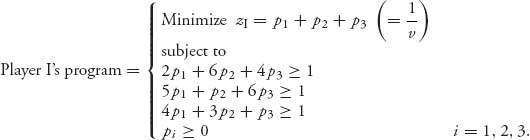
Example 9.2 Use the linear programming method to find a solution of the game with matrix
Since it is possible that the value of this game is zero, begin by making all entries positive by adding 4 (other numbers could also be used) to everything:
Here is player I’s program. We are looking for ![]() which will be found from the linear program. Setting
which will be found from the linear program. Setting ![]() player I’s problem is
player I’s problem is
After finding the pi’s, we will set
![]()
and then, v(A) = v − 4 is the value of the original game with matrix A, and v is the value of the game with matrix A′. Then xi = v, pi will give the optimal strategy for player I.
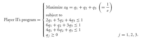
We next set up player II’s program. We are looking for y = (y1, y2, y3), yj ≥ 0, ![]() . Setting qj = (yj/v), player II’s problem is
. Setting qj = (yj/v), player II’s problem is
Having set up each player’s linear program, we now are faced with the formidable task of having to solve them. By hand this would be very computationally intensive, and it would be very easy to make a mistake. Fortunately, the simplex method is part of all standard Maple and Mathematica software so we will solve the linear programs using Maple.
For player I, we use the following Maple commands:
> with(simplex):
> cnsts:={2*p[1]+6*p[2]+4*p[3] >=1,
      *p[1]+p[2]+6*p[3] >=1, 4*p[1]+3*p[2]+p[3] >=1};
> obj:=p[1]+p[2]+p[3];
> minimize(obj, cnsts, NONNEGATIVE);
The minimize command incorporates the constraint that the variables be nonnegative by the use of the third argument. Maple gives the following solution to this program:
![]()
Unwinding this to the original game, we have
So, the optimal mixed strategy for player I, using xi = pi, v, is ![]() , and the value of our original game is
, and the value of our original game is ![]()
Next, we turn to solving the program for player II. We use the following Maple commands:
> with(simplex):
> cnsts:={2*q[1]+5*q[2]+4*q[3]<=1,
     6*q[1]+q[2]+3*q[3]<=1,
     4*q[1]+6*q[2]+q[3]<=1};
> obj:=q[1]+q[2]+q[3];
> maximize(obj, cnsts, NONNEGATIVE);
Maple gives the solution
![]()
so again ![]() Hence, the optimal strategy for player II is
Hence, the optimal strategy for player II is
The value of the original game is then ![]()
Remark As mentioned earlier, the linear programs for each player are the duals of each other. Precisely, for player I the problem is
where b = (1, 1, 1). The dual of this is the linear programming problem for player II:
The duality theorem of linear programming guarantees that the minimum in player I’s program will be equal to the maximum in player II’s program, as we have seen in this example.
Example 2.10 A Nonsymmetric Noisy Duel. We consider a nonsymmetric duel at which the two players may shoot at paces (10, 6, 2) with accuracies (0.2, 0.4, 1.0) each. This is the same as our previous duel, but now we have the following payoffs to player I at the end of the duel:
- If only player I survives, then player I receives payoff a.
- If only player II survives, player I gets payoff b < a. This assumes that the survival of player II is less important than the survival of player I.
- If both players survive, they each receive payoff zero.
- If neither player survives, player I receives payoff g.
We will take a = 1, b = ![]() , g = 0. Then here is the expected payoff matrix for player I:
, g = 0. Then here is the expected payoff matrix for player I:
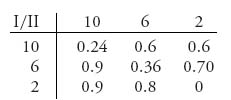
The pure strategies are (x, y), where x = 10, 6, 2 and y = 10, 6, 2. The elements of the matrix are obtained from the general formula
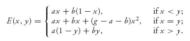
For example, if we look at
![]()
because if player II kills I at 10, then he survives and the payoff to I is b. If player II shoots, but misses player I at 10, then player I is certain to kill player II later and will receive a payoff of a. Similarly,
To solve the game, we use the Maple commands that will help us calculate the constraints:
> with(LinearAlgebra):
> R:=Matrix([[0.24, 0.6, 0.6], [0.9, 0.36, 0.70], [0.9, 0.8, 0]]);
> with(Optimization): P:=Vector(3, symbol=p);
> PC:=Transpose(P).R;
> Xcnst:={seq(PC[i]>=1, i = 1..3)};
> Xobj:=add(p[i], i = 1..3);
> Z:=Minimize(Xobj, Xcnst, assume=nonnegative);
> v:=evalf(1/Z[1]); for i from 1 to 3 do evalf(v*Z[2, i]) end do;
Alternatively, use the simplex package:
> with(simplex):Z:=minimize(Xobj, Xcnst, NONNEGATIVE);
Maple produces the output
![]()
This says that the value of the game is ![]() and the optimal strategy for player I is X* = (0.532, 0.329, 0.140). By a similar analysis of player II’s linear programming problem, we get Y* = (0.141, 0.527, 0.331). So player I should fire at 10 paces more than half the time, even though they have the same accuracy functions, and a miss is certain death. Player II should fire at 10 paces only about 14% of the time.
and the optimal strategy for player I is X* = (0.532, 0.329, 0.140). By a similar analysis of player II’s linear programming problem, we get Y* = (0.141, 0.527, 0.331). So player I should fire at 10 paces more than half the time, even though they have the same accuracy functions, and a miss is certain death. Player II should fire at 10 paces only about 14% of the time.
2.4.2 A DIRECT FORMULATION WITHOUT TRANSFORMING: METHOD 2
It is not necessary to make the transformations we made in order to turn a game into a linear programming problem. In this section, we give a simpler and more direct way. We will start from the beginning and recapitulate the problem.
Recall that player I wants to choose a mixed strategy X* = ![]() so as to
so as to
![]()
subject to the constraints
![]()
and
This is a direct translation of the properties (Section 1.3.1) that say that X* is optimal and v is the value of the game if and only if, when X* is played against any column for player II, the expected payoff must be at least v. Player I wants to get the largest possible v so that the expected payoff against any column for player II is at least v. Thus, if we can find a solution of the program subject to the constraints, it must give the optimal strategy for I as well as the value of the game.
Similarly, player II wants to choose a strategy Y* = (yj*) so as to
![]()
subject to the constraints
and
The solution of this dual linear programming problem will give the optimal strategy for player II and the same value of the game as that for player I. We can solve these programs directly without changing to new variables. Since we don’t have to divide by v in the conversion, we don’t need to ensure that v > 0 (although it is usually a good idea to do that anyway), so we can avoid having to add a constant to A. This formulation is much easier to set up in Maple, but if you ever have to solve a game by hand using the simplex method, the first method is much easier.
Let’s work an example and give the Maple commands to solve the game.
Example 2.11 In this example, we want to solve by the linear programming method with the second formulation the game with the skew symmetric matrix:
Here is the setup for solving this using Maple:
> with(LinearAlgebra):with(simplex):
> A:=Matrix([[0, -1, 1], [1, 0, -1], [-1, 1, 0]]);
>#The row player’s Linear Programming problem:
> X:=Vector(3, symbol= x);
> B:=Transpose(X).A;
> cnstx:={seq(B[i] >=v, i=1..3), seq(x[i] >= 0, i=1..3),
                                add(x[i], i=1..3)=1};
> maximize(v, cnstx);

>#Column players Linear programming problem:
> Y:=<y[1], y[2], y[3]>;#Another way to set up the vector for Y.
> B:=A.Y;
> cnsty:={seq(B[j]<=w, j=1..3), seq(y[j] >=0, j=1..3,
                                add(y[j], j=1..3)=1};
> minimize(w, cnsty);
Since A is skew symmetric, we know ahead of time that the value of this game is 0. Maple gives us the optimal strategies
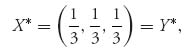
which checks with the fact that for a symmetric matrix the strategies are the same for both players.
Now let’s look at a much more interesting example.
Example 2.12 Colonel Blotto Games. This is a simplified form of a military game in which the leaders must decide how many regiments to send to attack or defend two or more targets. It is an optimal allocation of forces game. In one formulation from Karlin (1992), suppose that there are two opponents (players), which we call Red and Blue. Blue controls four regiments, and Red controls three. There are two targets of interest, say, A and B. The rules of the game say that the player who sends the most regiments to a target will win one point for the win and one point for every regiment captured at that target. A tie, in which Red and Blue send the same number of regiments to a target, gives a zero payoff. The possible strategies for each player consist of the number of regiments to send to A and the number of regiments to send to B, and so they are pairs of numbers. The payoff matrix to Blue is
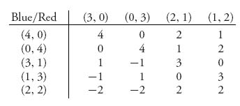
For example, if Blue plays (3, 1) against Red’s play of (2, 1), then Blue sends three regiments to A while Red sends two. So Blue will win A, which gives +1 and then capture the two Red regiments for a payoff of +3 for target A. But Blue sends one regiment to B and Red also sends one to B, so that is considered a tie, or standoff, with a payoff to Blue of 0. So the net payoff to Blue is +3.
This game can be easily solved using Maple as a linear program, but here we will utilize the fact that the strategies have a form of symmetry that will simplify the calculations and are an instructive technique used in game theory.
It seems clear from the matrix that the Blue strategies (4, 0) and (0, 4) should be played with the same probability. The same should be true for (3, 1) and (1, 3). Hence, we may consider that we really only have three numbers to determine for a strategy for Blue:
![]()
Similarly, for Red we need to determine only two numbers:
![]()
But don’t confuse this with reducing the matrix by dominance because that isn’t what’s going on here. Dominance would say that a dominated row would be played with probability zero, and that is not the case here. We are saying that for Blue rows 1 and 2 would be played with the same probability, and rows 3 and 4 would be played with the same probability. Similarly, columns 1 and 2, and columns 3 and 4, would be played with the same probability for Red. The net result is that we only have to find (x1, x2, x3) for Blue and (y1, y2) for Red.
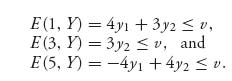
Red wants to choose y1 ≥ 0, y2 ≥ 0 to make value(A) = v as small as possible but subject to E(i, Y) ≤ v, i = 1, 3, 5. That is what it means to play optimally. This says
Now, 3y2 ≤ 4y1 + 3y2 ≤ v implies 3y2 ≤ v automatically, so we can drop the second inequality. Since 2y1 + 2y2 = 1, substitute y2= ![]() − y1 to eliminate y2 and get
− y1 to eliminate y2 and get
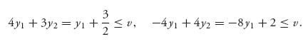
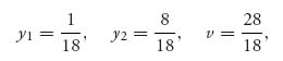
The two lines v = y1 + ![]() and v = −8y1 + 2 intersect at y1 =
and v = −8y1 + 2 intersect at y1 = ![]() , v =
, v = ![]() . Since the inequalities require that v be above the two lines, the smallest v satisfying the inequalities is at the point of intersection. Observe the connection with the graphical method for solving games. Thus,
. Since the inequalities require that v be above the two lines, the smallest v satisfying the inequalities is at the point of intersection. Observe the connection with the graphical method for solving games. Thus,
and Y* = (![]() ,
, ![]() ,
, ![]() ,
, ![]() ). To check that it is indeed optimal, we have
). To check that it is indeed optimal, we have
so that E(i, Y*) ≤ ![]() , i = 1, 2, …, 5. This verifies that Y* is optimal for Red.
, i = 1, 2, …, 5. This verifies that Y* is optimal for Red.
Next, we find the optimal strategy for Blue. We have E(3, Y*) = 3y2 = ![]() <
< ![]() and, because it is a strict inequality, property 4 of the Properties (Section 1.3.1), tells us that any optimal strategy for Blue would have 0 probability of using row 3, that is, x2 = 0. (Recall that X = (x1, x1, x2, x2, x3) is the strategy we are looking for.) With that simplification, we obtain the inequalities for Blue as
and, because it is a strict inequality, property 4 of the Properties (Section 1.3.1), tells us that any optimal strategy for Blue would have 0 probability of using row 3, that is, x2 = 0. (Recall that X = (x1, x1, x2, x2, x3) is the strategy we are looking for.) With that simplification, we obtain the inequalities for Blue as
In addition, we must have 2x1 + x3 = 1. The maximum minimum occurs at x1 = ![]() , x3 =
, x3 = ![]() , where the lines 2x1 + x3 = 1 and 3x1 + 2x3 =
, where the lines 2x1 + x3 = 1 and 3x1 + 2x3 = ![]() intersect. The solution yields X* = (
intersect. The solution yields X* = (![]() ,
, ![]() , 0, 0,
, 0, 0, ![]() ).
).
Naturally, Blue, having more regiments, will come out ahead, and a rational opponent (Red) would capitulate before the game even began. Observe also that with two equally valued targets, it is optimal for the superior force (Blue) to not divide its regiments, but for the inferior force to split its regiments, except for a small probability of doing the opposite.
Finally, if we use Maple to solve this problem, we use the following commands:
>with(LinearAlgebra):
>A:=Matrix([[4, 0, 2, 1], [0, 4, 1, 2], [1, -1, 3, 0], [-1, 1, 0, 3],
   [-2, -2, 2, 2]]);
>X:=Vector(5, symbol=x);
>B:=Transpose(X).A;
>cnst:={seq(B[i]>=v, i=1..4), add(x[i], i=1..5)=1};
>with(simplex):
>maximize(v, cnst, NONNEGATIVE, value);
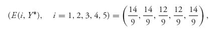
The outcome of these commands is X* = (![]() ,
, ![]() , 0, 0,
, 0, 0, ![]() ) and value = 14/9. Similarly, using the commands
) and value = 14/9. Similarly, using the commands
>with(LinearAlgebra):
>A:=Matrix([[4, 0, 2, 1], [0, 4, 1, 2], [1, -1, 3, 0], [-1, 1, 0, 3],
   [-2, -2, 2, 2]]);
>Y:=Vector(4, symbol=y);
>B:=A.Y;
>cnst:={seq(B[j]<=v, j=1..5), add(y[i], j=1..4)=1};
>with(simplex):
>minimize(v, cnst, NONNEGATIVE, value);
results in Y* = (![]() ,
, ![]() ,
, ![]() ,
, ![]() ) and again v =
) and again v = ![]() . The optimal strategy for Red is not unique, and Red may play one of many optimal strategies but all resulting in the same expected outcome. Any convex combination of the two Y*s we found will be optimal for player II.
. The optimal strategy for Red is not unique, and Red may play one of many optimal strategies but all resulting in the same expected outcome. Any convex combination of the two Y*s we found will be optimal for player II.
Suppose, for example, we take the Red strategy
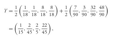
we get (E(i, Y), i = 1, 2, 3, 4, 5) = (![]() ,
, ![]() ,
, ![]() ,
, ![]() ,
, ![]() ). Suppose also that Blue deviates from his optimal strategy X* = (
). Suppose also that Blue deviates from his optimal strategy X* = (![]() ,
, ![]() , 0, 0,
, 0, 0, ![]() ) by using X =(
) by using X =(![]() ,
, ![]() ,
, ![]() ,
, ![]() ,
, ![]() ). Then E(X, Y) =
). Then E(X, Y) = ![]() < v =
< v = ![]() , and Red decreases the payoff to Blue.
, and Red decreases the payoff to Blue.
Problems
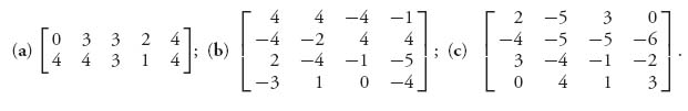
2.26 Use any method to solve the games with the following matrices.
2.27 Solve this game using the two methods of setting it up as a linear program:
In each of the following problems, set up the payoff matrices and solve the games using the linear programming method with both formulations, that is, both with and without transforming variables. You may use Maple/Mathematica or any software you want to solve these linear programs.
2.28 Consider the Submarine versus Bomber game. The board is a 3 × 3 grid.
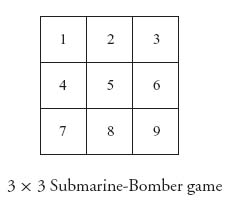
A submarine (which occupies two squares) is trying to hide from a plane that can deliver torpedoes. The bomber can fire one torpedo at a square in the grid. If it is occupied by a part of the submarine, the sub is destroyed (score 1 for the bomber). If the bomber fires at an unoccupied square, the sub escapes (score 0 for the bomber). The bomber should be the row player.
2.29 There are two presidential candidates, John and Dick, who will choose which states they will visit to garner votes. Suppose that there are four states that are in play, but candidate John only has the money to visit three states. If a candidate visits a state, the gain (or loss) in poll numbers is indicated as the payoff in the matrix
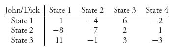
Solve the game.
2.30 Assume that we have a silent duel but the choice of a shot may be taken at 10, 8, 6, 4, or 2 paces. The accuracy, or probability of a kill is 0.2, 0.4, 0.6, 0.8, and 1, respectively, at the paces. Set up and solve the game.
2.31 Consider the Cat versus Rat game in Example 1.3. Suppose each player moves exactly three segments. The payoff to the cat is 1 if they meet and 0 otherwise. Find the matrix and solve the game.
2.32 Drug runners can use three possible methods for running drugs through Florida: small plane, main highway, or backroads. The cops know this, but they can only patrol one of these methods at a time. The street value of the drugs is $100, 000 if the drugs reach New York using the main highway. If they use the backroads, they have to use smaller-capacity cars so the street value drops to $80, 000. If they fly, the street value is $150, 000. If they get stopped, the drugs and the vehicles are impounded, they get fined, and they go to prison. This represents a loss to the drug kingpins of $90, 000, by highway, $70, 000 by backroads, and $130, 000 if by small plane. On the main highway, they have a 40% chance of getting caught if the highway is being patrolled, a 30% chance on the backroads, and a 60% chance if they fly a small plane (all assuming that the cops are patrolling that method). Set this up as a zero sum game assuming that the cops want to minimize the drug kingpins gains, and solve the game to find the best strategies the cops and drug lords should use.
2.33 LUC is about to play UIC for the state tennis championship. LUC has two players: A and B, and UIC has three players: X, Y, Z. The following facts are known about the relative abilities of the players: X always beats B; Y always beats A; A always beats Z. In any other match, each player has a probability ![]() of winning. Before the matches, the coaches must decide on who plays who. Assume that each coach wants to maximize the expected number of matches won (these are singles matches and there are two games so each coach must pick who will play game 1 and who will play game 2. The players do not have to be different in each game).
of winning. Before the matches, the coaches must decide on who plays who. Assume that each coach wants to maximize the expected number of matches won (these are singles matches and there are two games so each coach must pick who will play game 1 and who will play game 2. The players do not have to be different in each game).
Set this up as a matrix game. Find the value of the game and the optimal strategies.
2.34 Player II chooses a number j ![]() {1, 2, …, n}, n ≥ 2, while I tries to guess what it is by guessing an i
{1, 2, …, n}, n ≥ 2, while I tries to guess what it is by guessing an i ![]() {1, 2, …, n}. If the guess is correct (i.e., i = j) then II pays +1 to player I. If i > j player II pays player I the amount bi−j where 0 < b < 1 is fixed. If i < j, player I wins nothing.
{1, 2, …, n}. If the guess is correct (i.e., i = j) then II pays +1 to player I. If i > j player II pays player I the amount bi−j where 0 < b < 1 is fixed. If i < j, player I wins nothing.
2.35 Consider the asymmetric silent duel in which the two players may shoot at paces (10, 6, 2) with accuracies (0.2, 0.4, 1.0) for player I, but, since II is a better shot, (0.6, 0.8, 1.0) for player II. Given that the payoffs are +1 to a survivor and −1 otherwise (but 0 if a draw), set up the matrix game and solve it.
2.36 Suppose that there are four towns connected by a highway as in the following diagram:
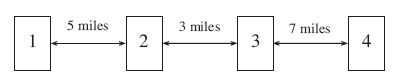
Assume that 15% of the total populations of the four towns are nearest to town 1, 30% nearest to town two, 20% nearest to town three, and 35% nearest to town four. There are two superstores, say, I and II, thinking about building a store to serve these four towns. If both stores are in the same town or in two different towns but with the same distance to a town, then I will get a 65% market share of business. Each store gets 90% of the business of the town in which they put the store if they are in two different towns. If store I is closer to a town than II is, then I gets 90% of the business of that town. If store I is farther than store II from a town, store I still gets 40% of that town’s business, except for the town II is in. Find the payoff matrix and solve the game.
2.37 Two farmers are having a fight over a disputed 6-yard-wide strip of land between their farms. Both farmers think that the strip is theirs. A lawsuit is filed and the judge orders them to submit a confidential settlement offer to settle the case fairly. The judge has decided to accept the settlement offer that concedes the most land to the other farmer. In case both farmers make no concession or they concede equal amounts, the judge will favor farmer II and award her all 6 yards. Formulate this as a constant sum game assuming that both farmers’ pure strategies must be the yards that they concede: 0, 1, 2, 3, 4, 5, 6. Solve the game. What if the judge awards 3 yards if there are equal concessions?
2.38 Two football teams, B and P, meet for the Superbowl. Each offense can play run right (RR), run left (RL), short pass (SP), deep pass (DP), or screen pass (ScP). Each defense can choose to blitz (Bl), defend a short pass (DSP), or defend a long pass (DLP), or defend a run (DR). Suppose that team B does a statistical analysis and determines the following payoffs when they are on defense:
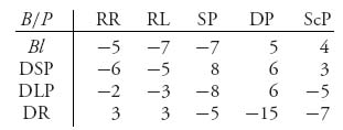
A negative payoff represents the number of yards gained by the offense, so a positive number is the number of yards lost by the offense on that play of the game. Solve this game and find the optimal mix of plays by the defense and offense. (Caution: This is a matrix in which you might want to add a constant to ensure v(A) > 0. Then subtract the constant at the end to get the real value. You do not need to do that with the strategies.)
2.39 Let a > 0. Use the graphical method to solve the game in which player II has an infinite number of strategies with matrix
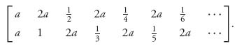
Pick a value for A and solve the game with a finite number of columns to see what’s going on.
2.40 A Latin square game is a square game in which the matrix A is a Latin square. A Latin square of size n has every integer from 1 to n in each row and column.
2.41 Consider the game with matrix 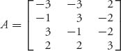
is not a saddle point of the game if 0 ≤ λ ≤ 1.
2.42 Two players, Curly and Shemp, are betting on the toss of a fair coin. Shemp tosses the coin, hiding the result from Curly. Shemp looks at the coin. If the coin is heads, Shemp says that he has heads and demands $1 from Curly. If the coin is tails, then Shemp may tell the truth and pay Curly $1, or he may lie and say that he got a head and demands $1 from Curly. Curly can challenge Shemp whenever Shemp demands $1 to see whether Shemp is telling the truth, but it will cost him $2 if it turns out that Shemp was telling the truth. If Curly challenges the call and it turns out that Shemp was lying, then Shemp must pay Curly $2. Find the matrix and solve the game.
2.43 Wiley Coyote5 is waiting to nab Speedy who must emerge from a tunnel with three exits, A, B, and C. B and C are relatively close together, but far away from A. Wiley can lie in wait for Speedy near an exit, but then he will catch Speedy only if Speedy uses this exit. But Wiley has two other options. He can wait between B and C, but then if Speedy comes out of A he escapes while if he comes out of B or C, Wiley can only get him with probability p. Wiley’s last option is to wait at a spot overlooking all three exits, but then he catches Speedy with probability q no matter which exit Speedy uses.
2.44 Left and Right bet either $1 or $2. If the total amount wagered is even, then Left takes the entire pot; if it is odd, then Right takes the pot.
Analyze each of these cases.
2.45 The evil Don Barzini has imprisoned Tessio and three of his underlings in the Corleone family (total value 4) somewhere in Brooklyn, and Clemenza and his two assistants somewhere in Queens (total value 3). Sonny sets out to rescue either Tessio or Clemenza and their associates; Barzini sets out to prevent the rescue but he doesn’t know where Sonny is headed. If they set out to the same place, Barzini has an even chance of arriving first, in which case Sonny returns without rescuing anybody. If Sonny arrives first he rescues the group. The payoff to Sonny is determined as the number of Corleone family members rescued. Describe this scenario as a matrix game and determine the optimal strategies for each player.
2.46 You own two companies Uno and Due. At the end of a fiscal year, Uno should have a tax bill of $3 million and Due should have a tax bill of $1 million. By cooking the books you can file tax returns making it look as though you should not have to pay any tax at all for either Uno or Due, or both. Due to limited resources, the IRS can only audit one company. If a company with cooked books is audited, the fraud is revealed and all unpaid taxes will be levied plus a penalty of p% of the tax due.
2.5 Appendix: Linear Programming and the Simplex Method
Linear programming is one of the major success stories of mathematics for applications. Matrix games of arbitrary size are solved using linear programming, but so is finding the best route through a network for every single telephone call or computer network connection. Oil tankers are routed from port to port in order to minimize costs by a linear programming method. Linear programs have been found useful in virtually every branch of business and economics and many branches of physics and engineering–even in the theory of nonlinear partial differential equations. If you are curious about how the simplex method works to find an optimal solution, this is the section for you. We will have to be brief and only give a bare outline, but rest assured that this topic can easily consume a whole year or two of study, and it is necessary to know linear programming before one can deal adequately with nonlinear programming.
The standard linear programming problem consists of maximizing (or minimizing) a linear function ![]() over a special type of convex set called a polyhedral set
over a special type of convex set called a polyhedral set ![]() , which is a set given by a collection of linear constraints
, which is a set given by a collection of linear constraints
where An×m is a matrix, ![]() is considered as an m × 1 matrix, or vector, and
is considered as an m × 1 matrix, or vector, and ![]() is considered as an n × 1 column matrix. The inequalities are meant to be taken componentwise, so x ≥ 0 means xj ≥ 0, j = 1, 2, …, m, and Ax ≤ b means
is considered as an n × 1 column matrix. The inequalities are meant to be taken componentwise, so x ≥ 0 means xj ≥ 0, j = 1, 2, …, m, and Ax ≤ b means
FIGURE 2.2 Extreme points of a convex set.
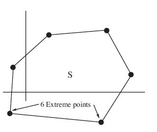
The extreme points of S are the key. Formally, an extreme point, as depicted in Figure 2.2, is a point of S that cannot be written as a convex combination of two other points of S; in other words, if x = λx1 + (1 − λ)x2, for some 0 < λ < 1, x1 ![]() S, x2
S, x2 ![]() S, then x = x1 = x2.
S, then x = x1 = x2.
Now here are the standard linear programming problems:
The matrix A is n × m, b is n × 1, and c is 1 × m. To get an idea of what is happening, we will solve a two-dimensional problem in the next example by graphing it.
Example 2.13 The linear programming problem is
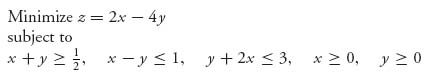
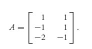
So c = (2, −4), b = (![]() , −1, −3) and
, −1, −3) and
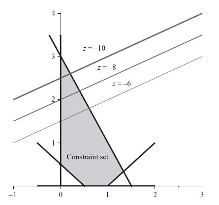
We graph (using Maple) the constraints, and we also graph the objective z = 2x − 4y = k on the same graph with various values of k as in Figure 2.3.
The values of k that we have chosen are k = −6, −8, −10. The graph of the objective is, of course, a straight line for each k. The important thing is that as k decreases, the lines go up. From the direction of decrease, we see that the furthest we can go in decreasing k before we leave the constraint set is at the top extreme point. That point is x = 0, y = 3, and so the minimum objective subject to the constraints is z = −12.
The simplex method of linear programming basically automates this procedure for any number of variables or constraints. The idea is that the maximum and minimum must occur at extreme points of the region of constraints, and so we check the objective at those points only. At each extreme point, if it does not turn out to be optimal, then there is a direction that moves us to the next extreme point and that does improve the objective. The simplex method then does not have to check all the extreme points, just the ones that improve our goal.
FIGURE 2.3 Objective plotted over the constraint set.
The first step in using the simplex method is to change the inequality constraints into equality constraints Ax = b, which we may always do by adding variables to x, called slack variables. So we may consider
![]()
We assume that S ≠ ![]() . We also need the idea of an extreme direction for S. A vector d ≠ 0 is an extreme direction of S if and only if A d = 0 and d ≥ 0. The simplex method idea then formalizes the approach that we know the optimal solution must be at an extreme point, so we begin there. If we are at an extreme point which is not our solution, then move to the next extreme point along an extreme direction. The extreme directions show how to move from extreme point to extreme point in the quickest possible way, improving the objective the most. Winston (1991) is a comprehensive resource for all of these concepts.
. We also need the idea of an extreme direction for S. A vector d ≠ 0 is an extreme direction of S if and only if A d = 0 and d ≥ 0. The simplex method idea then formalizes the approach that we know the optimal solution must be at an extreme point, so we begin there. If we are at an extreme point which is not our solution, then move to the next extreme point along an extreme direction. The extreme directions show how to move from extreme point to extreme point in the quickest possible way, improving the objective the most. Winston (1991) is a comprehensive resource for all of these concepts.
In Section 2.5.1, we will show how to use the simplex method by hand. We will not go into any more theoretical details as to why this method works, and simply refer you to Winston’s (1991) book.
2.5.1 THE SIMPLEX METHOD STEP BY STEP
We present the simplex method specialized for solving matrix games, starting with the standard problem setup for player II. The solution for player I can be obtained directly from the solution for player II, so we only have to do the computations once. Here are the steps. We list them first and then go through them so don’t worry about unknown words for the moment:
Look at all the numbers in the bottom row, excluding the answer column. From these, choose the largest number in absolute value. The column it is in is the pivot column. If there are two possible choices, choose either one. If all the numbers in the bottom row are zero or positive, then you are done. The basic solution is the optimal solution.
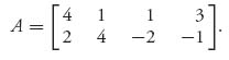
Here is a worked example following the steps. It comes from the game with matrix
We will consider the linear programming problem for player II. Player II’s problem is always in standard form when we transform the game to a linear program using the first method of Section 2.4. It is easiest to start with player II rather than player I.
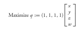
1. The problem is
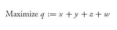
subject to
![]()
In matrix form this is
subject to
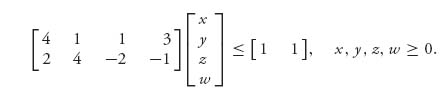
At the end of our procedure, we will find the value as v(A) = ![]() , and the optimal strategy for player II as Y* = v(A)(x, y, z, w). We are not modifying the matrix because we know ahead of time that v(A) ≠ 0. (Why? Hint: Calculate v−.)
, and the optimal strategy for player II as Y* = v(A)(x, y, z, w). We are not modifying the matrix because we know ahead of time that v(A) ≠ 0. (Why? Hint: Calculate v−.)
We need two slack variables to convert the two inequalities to equalities. Let’s call them s, t ≥ 0, so we have the equivalent problem
![]()
subject to

The coefficients of the objective give us the vector c = (1, 1, 1, 1, 0, 0). Now we set up the initial tableau.
2. Here is where we start:
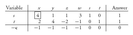
This is the initial tableau.
3. The pivot column is the column with the smallest number in the last row, i.e., the row for −c. Since we have several choices for the pivot column (because there are four −1s), we choose the first column arbitrarily. Note that the last row uses c, not c, because the method is designed to minimize, but we are actually maximizing here.
4. We choose the pivot in the first column by looking at the ratios ![]() , where A is the number in the answer column and b is the number in the pivot column, for each row not including the bottom row. This gives
, where A is the number in the answer column and b is the number in the pivot column, for each row not including the bottom row. This gives ![]() and
and ![]() with the smaller ratio
with the smaller ratio ![]() . This means that the 4 in the second column is the pivot element.
. This means that the 4 in the second column is the pivot element.
5. Now we row reduce the tableau using the 4 in the first column until all the other numbers in that column are zero. Here is the next tableau after carrying out those row operations:
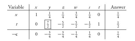
Note that on the leftmost (first) column we have replaced the variable s with the variable x to indicate that the s variable is leaving (has left) and the x variable is entering.
6. We repeat the procedure of looking for a pivot column. We have a choice of choosing either column with the ![]() on the bottom. We choose the first such column because if we calculate the ratios we get (
on the bottom. We choose the first such column because if we calculate the ratios we get (![]() )/(
)/(![]() ) = 1 and (
) = 1 and (![]() )/(
)/(![]() ) =
) = ![]() , and that is the smallest ratio. So the pivot element is the
, and that is the smallest ratio. So the pivot element is the ![]() in the third column.
in the third column.
After row reducing on the pivot ![]() , we get the next tableau.
, we get the next tableau.
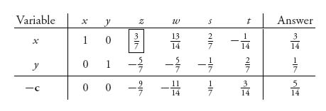
The slack variable t has left and the variable y has entered.
7. The largest element in the bottom row is −![]() so that is the pivot column. The pivot element in that column must be
so that is the pivot column. The pivot element in that column must be ![]() because it is the only positive number left in the column. So, we reduce row on the
because it is the only positive number left in the column. So, we reduce row on the ![]() pivot and finally end up with the tableau.
pivot and finally end up with the tableau.
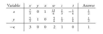
We have reached the end. All of the numbers on the bottom row are nonnegative so we are done. Now we read off the solution.
The maximum objective is in the lower right corner, q = 1.
The maximum is achieved at the variables z = ![]() , y =
, y = ![]() , x = 0, w = 0, because the z and y variables are on the left column and equal the corresponding value in the answer column. The remaining variables are zero because they are not in the variable column.
, x = 0, w = 0, because the z and y variables are on the left column and equal the corresponding value in the answer column. The remaining variables are zero because they are not in the variable column.
We conclude that v(A) = ![]() = 1, and Y* = (0,
= 1, and Y* = (0, ![]() ,
, ![]() , 0) is optimal for player II.
, 0) is optimal for player II.
To determine X*, we write down the dual of the problem for player II:
![]()
subject to
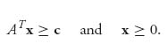
For convenience let’s match this up with player II’s problem:
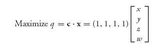
subject to
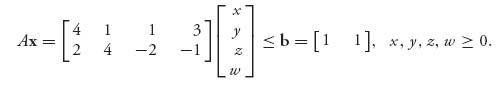
Note that to find the dual, the cost vector is replaced by the right-hand vector of the inequality constraints for player II, we replace A by AT, and the original cost vector c becomes the inequality constraints.
We could set up the simplex method for player I and solve it, but the solution is already present in the solution for player II; that is, the solution of the dual is already present in the final tableau of the primal. Ain’t math wonderful! For example, we computed, when we get to the final tableau, the optimal objective for the dual is the same as the primal (that is the duality theorem), but the optimal variables are in the bottom row corresponding to the columns headed by the slack variables! That means that v(A) = 1/q = 1 and X* = (1, 0), the 1 coming from s and the 0 coming from t. That’s it. We are done.
Now let’s check our answer by solving the game directly. If you look at the game matrix
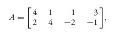
it is obvious that column 3 dominates all the other columns and so there is a saddle point at row 1, column 3. The saddle is X* = (1, 0) and Y* = (0, 0, 1, 0). In fact, there are an infinite number of optimal strategies for player II:
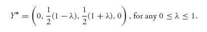
The simplex method gave us one of them.
Here is one last example.
Example 2.14 There are two presidential candidates, Harry and Tom, who will choose which states they will visit to garner votes. Their pollsters estimate that if, for example, Tom goes to state 2 and Harry goes to state 1, then Tom will lose 8 percentage points to Harry in that state. Suppose that there are three states that each candidate can select. Here is the matrix with Tom as the row player:
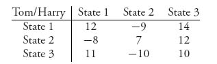
Each player wants to know which visits to which states he should make and what will be the net result. This is a game. There is an obvious dominance that allows us to drop state 3 for both players, but we will ignore this to see if we end up with that in our solution. That would be a quick check to see if everything works.
So, we have two methods to solve this problem. We could use the invertible matrix formulas and see if that works, or we could use linear programming, which is our choice here.
Step one is to set up the linear program for player II:
![]()
subject to
![]()
and q1, q2, q3 ≥ 0.
Next, we set up the initial tableau, which will have three slack variables because we have three inequality constraints:
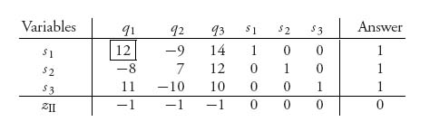
Instead of labeling the last row −c, we are labeling it with the objective value zII to keep track of the player number.
After pivoting on the 12 in the second column, we replace s1 by q1 in the first column:
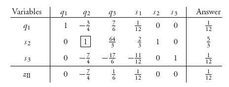
Finally, we pivot on the 1 in the third column and arrive at the final tableau:
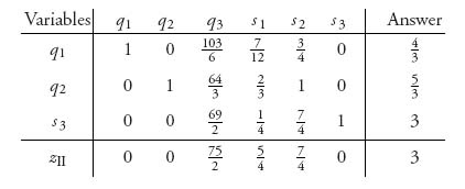
This is the final tableau because all numbers on the bottom are nonnegative. Note, too, that s2 in the first column was replaced by q2 because that was the pivot column.
Now we read off the information:
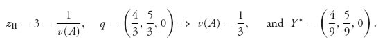
For player I, we look at the numbers under the slack variables in the final tableau, namely, ![]() ,
, ![]() , 0. This is the solution to the dual problem. In other words, the optimal solution for player I is p = (
, 0. This is the solution to the dual problem. In other words, the optimal solution for player I is p = (![]() ,
, ![]() , 0), which gives us
, 0), which gives us
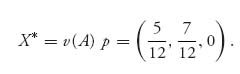
Sure enough, state 3 is never to be visited by either Tom or Harry. Tom should visit state 1, 5 out of 12 times and state 2, 7 out of 12 times. Interestingly, Harry should visit state 1, 4 out of 9 times and state 2, 5 out of 9 times. Tom ends up with a net gain of v(A) = 0.33%. It hardly seems worth the effort (unless the opponent doesn’t play optimally).
Of course, you can check these results with the following Maple commands:
> with (LinearAlgebra):
> value:=proc(A, rows, cols)
    local X, Y, B, C, cnstx, cnsty, vI, vII, vu, vl;
    X:=Vector(rows, symbol=x):
    Y:=Vector(cols, symbol=y):
    B:=Transpose(X).A; C:=A.Y;
    cnsty:={seq(C[j]<=vII, j=1..rows), add(y[j], j=1..cols)=1}:
    cnstx:={seq(B[i]>=vI, i=1..cols), add(x[i], i=1..rows)=1}:
    with(simplex):
    vu:=maximize(vI, cnstx, NONNEGATIVE);
    vl:=minimize(vII, cnsty, NONNEGATIVE);
    print(vu, vl);
  end:

> City:=Matrix([[12, -9, 14], [-8, 7, 12], [11, -10, 10]]);
> value(City, 3, 3);
These Maple commands produce the following output:
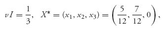
and
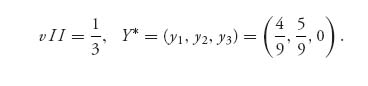
Problems
2.47 Use the simplex method to solve the games with the following matrices. Check your answers using Maple and verify that the strategies obtained are indeed optimal.
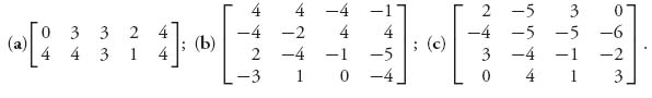
2.48 Solve this problem using Maple in two ways:
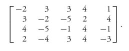
2.6 Review Problems
Give the precise definition, complete the statement, or answer True or False. If False, give the correct statement.
2.49 Complete the statement: In order for (X*, Y*) to be a saddle point and v to be the value, it is necessary and sufficient that E(X*, j)________, for all and ________E(i, Y*)________for all________.
2.50 State the von Neumann Minimax theorem for two person zero sum games with matrix A.
2.51 Suppose (X*, Y*) is a saddle point, v(A) is the value of the game and xk > 0 for the kth component of X*. What is E(k, Y*)? What is the most you can say if xk = 0 for E(k, Y*)?
2.52 Suppose A is a game matrix and Y0 is a given strategy for player II. Define what it means for X* to be a best response strategy to Y0 for player I.
2.53 Suppose An×n has an inverse A−1. What three assumptions do you need to be able to use the formulas
![]()
to conclude that v = v(A) and (X*, Y*) are optimal mixed strategies?
2.54 v(A) is the value and (X*, Y*) is a saddle point of the game with matrix A if and only if ….
2.55 v(A) is the value and (i*, j*) is a pure saddle point of the game with matrix A if and only if ….
2.56 For any game v+ ≤ v(A) ≤ v−.
2.57 For any matrix game E(X, Y) = X AYT and the value satisfies
v(A) = maxX minY E(X, Y) = minY maxX E(X, Y).
2.58 If (X*, Y*) is a saddle point for a matrix game, then X* is a best response strategy to Y* for player I, but the reverse is not necessarily true.
2.59 If Y is an optimal strategy for player II in a zero sum game and E(i, Y) < value(A) for some row i, then for any optimal strategy X for player I, we must have ….
2.60 The graphical method for solving a 2 × m game won’t work if ….
2.61 (X*, Y*) is a saddle point if and only if minj=1, 2, …, m E(X*, j) = maxi=1, 2, …, n E(i, Y*).
2.62 If (Y0, X0) is a saddle point for the game A, then E(Y0, X) ≥ E(Y0, X0) ≥ E(Y, X0), for all strategies X for player II and Y for player I.
2.63 If X* = ![]() is an optimal strategy for player I and
is an optimal strategy for player I and ![]() , then we may drop row 1 when we look for the optimal strategy for player II.
, then we may drop row 1 when we look for the optimal strategy for player II.
2.64 For a game matrix An×m and given strategies (X* = (x1, …, xn), Y* = (y1, …, ym), then ![]()
2.65 If i* = 2, j* = 3, is a pure saddle point in the game with matrix A3×4, then using mixed strategies, X* =_______________, Y* =______________ is a mixed saddle point for A.
2.66 For a 2 × 2 game with matrix ![]() , the value of the game is
, the value of the game is ![]() , where
, where ![]() .
.
2.67 The invertible matrix theorem says that if A−1 exists, then ![]() is the value of the game.
is the value of the game.
2.68 If f(x, y) = (x, 1 − x)![]() , then a mixed saddle point for the game X* = (x*, 1 − x*), Y* = (y*, 1 − y*), 0 < x*, y* < 1, satisfies
, then a mixed saddle point for the game X* = (x*, 1 − x*), Y* = (y*, 1 − y*), 0 < x*, y* < 1, satisfies
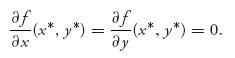
2.69 If A is a skew symmetric game with v(A) > 0, then there is always a saddle point in which X* = −Y*.
2.70 If A is skew symmetric then for any strategy X for player I, E(X, X) = 0.
2.7 Maple/Mathematica
2.7.1 Invertible Matrices
Here are the Maple commands to work out any invertible matrix game. You can try many different constants to add to the matrix to see if you get an inverse if the original matrix does not have an inverse.
> restart:with(LinearAlgebra):
> A:=Matrix([[0, 1, -2 ], [-1, -2, 3], [2, -3, -4 ]]);
> Determinant(A);
> A:=MatrixAdd(ConstantMatrix(-1, 3, 3), A);
> Determinant(A);
> B:=A ^ (-1);
> J:=Vector[row]([1, 1, 1 ]);
> J.B.Transpose(J);
> v:=1/(J.B.Transpose(J));
> X:=v*(J.B);
> Y:=v*(B.Transpose(J));
The first line loads the LinearAlgebra package. The next line enters the matrix. The Determinant command finds the determinant of the matrix so you can see if it has an inverse. The MatrixAdd command adds the constant 3 × 3 matrix that consists of all −1s to A. The ConstantMatrix(-1, 3, 3) says the matrix is 3 × 3 and has all −1s. If the determinant of the original matrix A is not zero, you change the MatrixAdd command to A:=MatrixAdd(ConstantMatrix(0, 3, 3), A). In general, you keep changing the constant until you get tired or you get an invertible matrix.
The inverse of A is put into the matrix B, and the row vector consisting of 1s is put into J. Finally, we calculate v = value(A) and the optimal mixed strategies X, Y.
In this particular example, the determinant of the original matrix is −12, but we add −1 to all entries anyway for illustration. This gives us v = −![]() , X = (
, X = (![]() ,
, ![]() ,
, ![]() ), and Y = (
), and Y = (![]() ,
, ![]() ,
, ![]() ), and these are legitimate strategies. So X and Y are optimal and the value of the original game is v(A) = −
), and these are legitimate strategies. So X and Y are optimal and the value of the original game is v(A) = −![]() + 1 = −
+ 1 = −![]() .
.
2.7.2 LINEAR PROGRAMMING: METHOD 1
We may also use the Optimization package in Maple to solve player I’s program, but this solves the problem numerically rather than symbolically. To use this package and solve the problem, use the following commands:
The matrix is 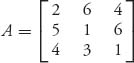 .
.
Player I
> with(Optimization):
> cnsts:={2*p[1]+6*p[2]+4*p[3] >=1,
          5*p[1]+p[2]+6*p[3] >=1,
          4*p[1]+3*p[2]+p[3] >=1};
> obj:=p[1]+p[2]+p[3];
> Minimize(obj, cnsts, assume=nonnegative);
This will give the solution in floating-point form: p[1] = 0.169, p[2] = 0.1048, p[3] = 0.00806. The minimum objective is 0.169 + 0.1048 + 0.00806 = 0.28186 and so the value of the game is v = 1/0.28186 − 4 = −0.457.
Player II
Solving the program for player II. We use the following Maple commands:
> with(Optimization):
> cnsts:={2*q[1]+5*q[2]+4*q[3]<=1,
          6*q[1]+q[2]+3*q[3]<=1,
          4*q[1]+6*q[2]+q[3]<=1};
> obj:=q[1]+q[2]+q[3];
> Maximize(obj, cnsts, assume=nonnegative);
Maple gives the solution q1 = 0.1048, q2 = 0.0806, q3 = 0.0967, with optimal objective 0.2822.
2.7.2.1 Mathematica for Both Players: Method 1 We present the Mathematica commands for solving the game with Mathematica. Here is method 1 that transforms variables:
Method1[Matrix_]:= Module[{matrix = Matrix, minEntry, constr1,
                           constr2, pi, qj, rowDim, colDim, X, Y, v},
minEntry = Min[matrix];
origmatrix=matrix;
(*This will guarantee that v != 0*)
If[minEntry <= 0, matrix = matrix + Abs[minEntry]+1, minEntry = -1];
rowDim = Dimensions[matrix][[1]];
colDim = Dimensions[matrix][[2]];
(*Solve the game*)
X=LinearProgramming[Table[1, {i, 1, rowDim}],
                       Transpose[matrix], Table[1, {i, 1, colDim}]];
Y = LinearProgramming[-Table[1, {i, 1, colDim}],
                       matrix, Table[{1, -1}, {i, 1, rowDim}]];
v = 1/Total[X];
(*Print the optimal strategies and the value of the game*)
Print[MatrixForm[origmatrix]];
Print["X = " <>ToString[v*X, FormatType-> StandardForm]];
Print["Y = " <>ToString[v*Y, FormatType-> StandardForm]];
Print["v = " <> ToString[v-(Abs[minEntry]+1), FormatType->
   StandardForm]];
];
2.7.3 LINEAR PROGRAMMING: METHOD 2
The matrix is 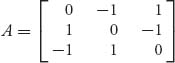 . The commands for both players are as follows:
> with(LinearAlgebra):with(simplex):
> A:=Matrix([[0, -1, 1], [1, 0, -1], [-1, 1, 0]]);

>#The row player’s Linear Programming problem:
> X:=Vector(3, symbol= x);
> B:=Transpose(X).A;
> cnstx:={seq(B[i] >=v, i=1..3), seq(x[i] >= 0, i=1..3),
                                add(x[i], i=1..3)=1};
> maximize(v, cnstx);

>#Column players Linear programming problem:
> Y:=<y[1], y[2], y[3]>;#Another way to set up the vector for Y.
> B:=A.Y;
> cnsty:={seq(B[j]<=w, j=1..3), seq(y[j] >=0, j=1..3,
                                add(y[j], j=1..3)=1};
> minimize(w, cnsty);
Remark The Maple commands for solving a game may be automated somewhat by using a Maple procedure:
>restart:with(LinearAlgebra):
>A:=Matrix([[4, 0, 2, 1], [0, 4, 1, 2], [1, -1, 3, 0], [-1, 1, 0, 3], [-2, -2, 2, 2]]);
>value:=proc(A, rows, cols)
    local X, Y, B, C, cnstx, cnsty, vI, vII, vu, vl;
    X:=Vector(rows, symbol=x): Y:=Vector(cols, symbol=y):
    B:=Transpose(X).A; C:=A.Y;
    cnsty:={seq(C[j]<=vII, j=1..rows), add(y[j], j=1..cols)=1,
    seq(y[j]>=0, j=1..cols)}:
    cnstx:={seq(B[i]>=vI, i=1..cols), add(x[i], i=1..rows)=1,
    seq(x[i]>=0, i=1..rows)}:
    with(simplex):
    vu:=maximize(vI, cnstx);
    vl:=minimize(vII, cnsty);
    print(vu, vl);
    end:
>value(A, 5, 4);
You may now enter the matrix A and run the procedure through the statement
value(A, rows, columns).
The procedure will return the value of the game and the optimal strategies for each player. In all cases, you should verify that you actually have the value of the game and the optimal strategies by using the verification: (X*, Y*) is a saddle point and v is the value if and only if
![]()
for every i = 1, 2, …, n, j = 1, 2, …, m.
2.7.3.1 Mathematica for Both Players: Method 2 Method 2 for solving a game using mathematica is very straightforward:
Method2[Matrix_]:= Module[{matrix=Matrix, rowDim, colDim, xi, yj,
                           constr1, constr2, soln1, soln2},
Clear[x, y, v];
rowDim = Dimensions[matrix][[1]];
colDim = Dimensions[matrix][[2]];
(*Get the symbolic constraints to display*)
xi = Table[Subscript[x, i], i, 1, rowDim];
yj = Table[Subscript[y, i], i, 1, colDim];
constr1 = Transpose[matrix].xi;
constr2 = matrix.yj;
constr1 = Map[# >= v&, constr1];
constr2 = Map[# <= v&, constr2];
(*Solve the game*)
soln1=Maximize[Prepend[Join[constr1, {Total[xi]==1,
                                       Map[#>= 0&, xi]}], v], Prepend[xi, v]];
soln2=Minimize[Prepend[Join[constr2, {Total[yj]==1,
                                       Map[#>= 0&, yj]}], v], Prepend[yj, v]];
Print[soln1];
Print[MatrixForm[matrix]]
Print[soln2];
  ];

To run this enter the matrix:

A={1, 3, 5}, {-1, 7, -2}, {2, -4, 1};
Method2[A];
Bibliographic Notes
Invertible matrices are discussed by Owen (2001) and Ferguson (2013) and in many other references. Symmetric games were studied early in the development of the theory because it was shown (see Problem 2.25, from Karlin (1992)) that any matrix game could be symmetrized so that techniques developed for symmetric games could be used to yield information about general games. Before the advent of high-speed computers, this was mostly of theoretical interest because the symmetrization made the game matrix much larger. Today, this is not much of a problem.
The introduction of the Burr–Hamilton duel is an example of a game of timing that is properly considered in the continuous-time setting discussed in later chapters. For the full generality, see Karlin’s (1992) book.
The fundamental idea of using linear programming to solve games, and the use of the duality theorem to even prove the existence of value of a matrix game, might have been known to several mathematicians at the same time. The exact originator of this idea is unknown to the present author but possibly may be due to Dantzig, von Neumann, Karlin, or others.
Problem 2.36 is a classic example of the use of game theory in a business problem. Here, it is used to determine the location of a business depending on marketing conditions and the location of a competitor’s store. Versions of this problem appear throughout the literature, but this version is due to R. Bronson. Problem 2.37 is an example of a dispute resolution problem (refer to Winston’s (1991) book) presaging the idea of cooperative games considered in Chapter 6. Problem 2.39 is an instructive problem on the use of the graphical method and appears in at least the books by Karlin (1992) and Jones (2000). The Colonel Blotto game is an early application of game theory to military theory. There is an entire class of games known as Blotto games. The analysis presented in Example 2.12 is due to Karlin and shows the techniques involved to solve an important game without the use of linear programming.
The use of the simplex method for solving matrix games by hand or by computer is standard and appears in almost all books on game theory. Here, we follow Ferguson’s approach in Ferguson (2013) because, as is pointed out in those notes, by starting with the program for player II, the solution for player I can be read off of the final tableau. This approach requires the transformation of the game into a linear programming problem by the first method.
1 The calculus definition of a saddle point of a function f(x, y) is a point so that in every neighborhood of the point there are x and y values that make f bigger and smaller than f at the candidate saddle point.
2 A Rand corporation mathematician and game theorist (1911–1992).
3 George Bernard Dantzig was born on November 8, 1914, and died May 13, 2005. He is considered the “father of linear programming.” He was the recipient of many awards, including the National Medal of Science in 1975, and the John von Neumann Theory Prize in 1974.
4 In 1947 Dantzig met with von Neumann and began to explain the linear programming model “as I would to an ordinary mortal.” After a while von Neumann ordered Dantzig to “get to the point.” Dantzig relates that in “less than a minute I slapped the geometric and algebraic versions …on the blackboard.” Von Neumann stood up and said “Oh, that.” Dantzig relates that von Neumann then “proceeded to give me a lecture on the mathematical theory of linear programs.” This story is related in the excellent article by Cottle, Johnson, and Wets in the Notices of the A.M.S., March 2007.
5 Versions of this and the remaining problems appeared on exams at the London School of Economics.