Problem Solutions
Solutions for Chapter 1
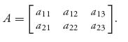
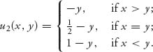
1.1 Think of this as a 100 × 100 game matrix and we are looking for the upper and lower values except that we are really doing it for the transpose of the matrix.
If we take the maximum in each row and then Javier is the minimum maximum, Javier is v+. If we take the minimum in each column, and Raoul is the maximum of those, then Raoul is the maximum minimum, or v−. Thus, Javier is richer.
Another way to think of this is that the poorest rich guy is wealthier than the richest poor guy. Common sense.
1.3.a The rock-paper-scissors game matrix with the rules of the problem is
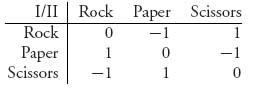
1.3.b v+ = 1, v− = −1. No saddle point in pure strategies since v+ > v−.
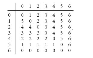
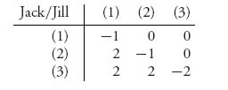
1.5 For each player we let (i, j) be the pure strategy in which the player shows i fingers, and guesses the other player will show j fingers. The matrix is
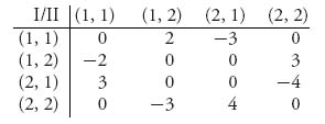
Since v+ = 2, v− = − 2, there are no pure optimal strategies.
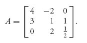
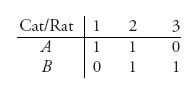
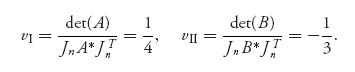
1.7 Consider first the game with A. To calculate v− we take the minimum of x and 0, written as { x, 0 }, and the minimum of 1, 2, which is 1. Then
![]()
since min { x, 0 } ≤ 0, no matter what x is. Similarly,
![]()
Thus, v− = v+ = 1 and there is a pure saddle at row 2, column 1.
For matrix B, we have v− = max { 1, min { x, 0 } } = 1, v+ = min { max { 2, x }, 1 } = 1, and there is a pure saddle at row 1, column 2, no matter what x is.
1.9 We have
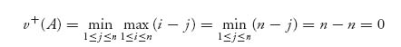
and
![]()
Thus, v = 0 with a pure saddle point at (n, n).
1.11 v+ = 1, v− = 0 because there is always at least one 1 and one 0 in each row and column.
11.13 Denote the game matrix as
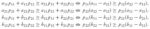
Without loss of generality, we may as well assume that the saddle is at row 1, column 1, v− = v+ = a11. Since (1, 1) is a saddle, we have
![]()
In particular, a21 ≤ a11. If it is also true that a22 ≤ a12 and a23 ≤ a13 then row 1 dominates row 2 and we are done. Thus, we need only suppose that a22 > a12. Then, from the saddle point inequalities,
![]()
But then a12 ≥ a11 and a22 > a21 says that column 2 is dominated by column 1.
Now consider the 3 × 3 matrix
Then v− = v+ = 1 and there is a saddle at row 2, column 3, but no row or column dominates another.
1.15.a The upper value is
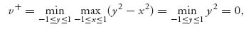
and the lower value is
![]()
since if y chooses first, y can choose y = x. Thus, v+ = 0, v− = 0.
1.15.b We have f(0, 0) = 0, and
![]()
1.17 Let x, ξ ![]()
![]() n, and α, β
n, and α, β ![]()
![]() . Then
. Then
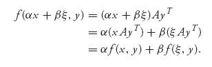
This proves x ![]() f(x, y) is linear. Similarly, y
f(x, y) is linear. Similarly, y ![]() f(x, y) is also linear.
f(x, y) is also linear.
1.19 Under the assumptions,
![]()
Then
![]()
Similarly,
and then
Since min max ≥ max min, we have from
that we must have equality throughout.
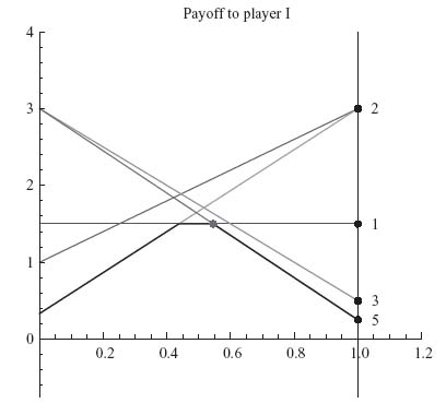
1.21 Since player II wants to guarantee that player I gets the smallest maximum, look at the line segments that are the highest and then choose the y* that gives the smallest maximum payoff. The point of intersection of the two lines is where the y* will be located and the corresponding horizontal coordinate will be the value of the game.
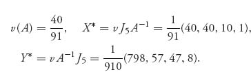
The result for this problem is 3y + 2(1 − y) = y + 4(1 − y), which implies that y* = ![]() and v(A) =
and v(A) = ![]() .
.
1.23 Let Curly be the row player and the thief be the column player. The matrix is
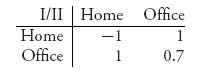
The payoff of 0.7 to Curly if he puts the gold bar at the office and the thief hits the office is obtained by calculating (+ 1)× 0.85 + (−1) × 0.15 = 0.7. The two lines for the expected payoffs of player I cross where E((x, 1 − x), 1) = E((x, 1 − x), 2), which becomes − x + (1 − x) = x + 0.7(1 − x). The solution is x* = ![]() .
.
Similarly, for player II the lines cross where E(1, (y, 1 − y)) = E(2, (y, 1 − y)), or − y + (1 − y) = y + 0.7(1 − y).
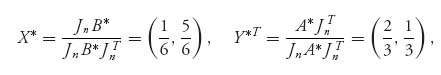
The mixed strategy solution is X* = Y* = (![]() ,
, ![]() ), v =
), v = ![]() .
.
1.25 Column 2 may be eliminated by dominance. Any ![]() ≤ λ ≤
≤ λ ≤ ![]() will make
will make
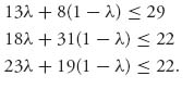
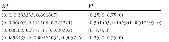
Once column 2 is gone, row 1 may be dropped. Then we apply the graphical method to get X* = (0, ![]() ,
, ![]() ) and Y* = (
) and Y* = (![]() , 0,
, 0, ![]() ). The value of the game is v =
). The value of the game is v = ![]() .
.
1.27 The game matrix is
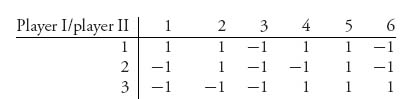
Column 3 immediately dominates every other column. Then it doesn’t matter what row player I chooses because the payoff is always −1.
1.29 (a) X* = (![]() ,
, ![]() ); (b) Y* = (
); (b) Y* = (![]() ,
, ![]() ); (c) Y* = (
); (c) Y* = (![]() ,
, ![]() ).
).
To see where these come from since they are all 2 × 2 games without pure saddle points, simply find where the two payoff lines cross for each player.
For (a) we must solve 4x − 9(1 − x) = − 3x + 6(1 − x) ![]() x =
x = ![]() , and 4y − 3(1 − y) = − 9y + 6(1 − y), which gives y =
, and 4y − 3(1 − y) = − 9y + 6(1 − y), which gives y = ![]() . Then plugging in to either payoff line we get v = −
. Then plugging in to either payoff line we get v = − ![]() . The other parts are similar.
. The other parts are similar.
1.31 Any ![]() ≤ λ ≤
≤ λ ≤ ![]() will work for a convex combination of columns 2 and 1. To see why
will work for a convex combination of columns 2 and 1. To see why
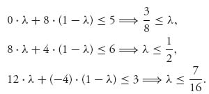
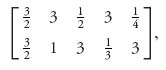
The reduced matrix is  . The graph for this matrix for player II is
The solution of the original game is, therefore, X* = (![]() ,
, ![]() , 0), Y* = (
, 0), Y* = (![]() ,
, ![]() , 0) and v(A) =
, 0) and v(A) = ![]() .
.
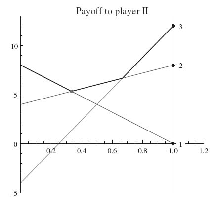
1.33 Column 2 is dominated by column 3, then row 3 is dominated by row 1. The reduced matrix is  which does not have a pure saddle. The resulting solution is obtained where the payoff lines cross; for example, a4 x + a1 (1 − x) = a3 x + a5 (1 − x)
 ![]() x* =
x* = ![]() We have
We have
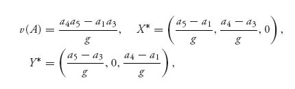
where g = a4 + a5 a1 − a3.
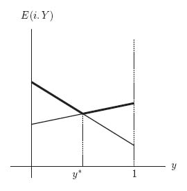
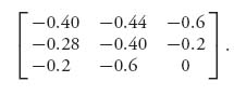
1.35.a The given strategies are not optimal because maxi E(i, Y) = ![]() and minj E(X, j) = −
and minj E(X, j) = − ![]() . Another way to see it, is to note that since rows 1 and 3 are used with positive probability, and Theorem 1.3.8 tells us that if X* is optimal we must have E(1, Y*) = E(3, Y*) = v, which you can check easily is not true. Similarly, since columns 2 and 3 are used with positive probability, it must be true that E(X*2) = E(X*, 3) for X* to be optimal. But that fails also. Neither X* nor Y* are optimal.
. Another way to see it, is to note that since rows 1 and 3 are used with positive probability, and Theorem 1.3.8 tells us that if X* is optimal we must have E(1, Y*) = E(3, Y*) = v, which you can check easily is not true. Similarly, since columns 2 and 3 are used with positive probability, it must be true that E(X*2) = E(X*, 3) for X* to be optimal. But that fails also. Neither X* nor Y* are optimal.
1.35.b The optimal Y* is Y* = ![]() This is obtained from solving the equations
This is obtained from solving the equations
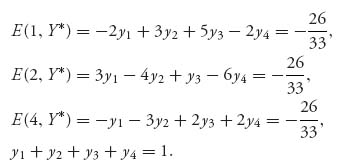
We use the fact that E(i, Y*) = v if xi* > 0.
1.37.a X* = (![]() ,
, ![]() ), Y* = (
), Y* = (![]() ,
, ![]() ), v(A) =
), v(A) = ![]() .
.
1.37.b Solving for the offense, we see that 3x + 12(1 − x) = 6x, which gives x* = ![]() , so the optimal strategy is X* = (
, so the optimal strategy is X* = (![]() ,
, ![]() ). The value of the game is v(A) =
). The value of the game is v(A) = ![]() and the optimal strategy for the defense is Y* = (
and the optimal strategy for the defense is Y* = (![]() ,
, ![]() ). If the offense gets a better quarterback, the team should run more!
). If the offense gets a better quarterback, the team should run more!
1.39.a The game matrix is
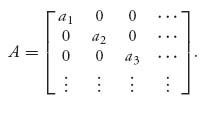
Then since there is a 0 in every row and all the ak′ s > 0, the maximum minimum must be v− = 0. Since there is an ak > 0 in every column, the maximum in every column is ak. The minimum of those is a1 and so v+ = a1.
1.39.b We use E(i, Y*) ≤ v ≤ E(X*, j), ∀ i, j = 1, 2, …. We get for X* = (x1, x2, …), E(X*, j) = aj xj ≥ v ![]() xj ≥
xj ≥ ![]() . Similarly, for Y* = (y1, y2, …), yj ≤
. Similarly, for Y* = (y1, y2, …), yj ≤ ![]() . Adding these inequalities results in
. Adding these inequalities results in
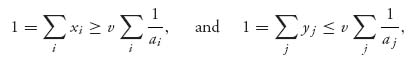
and we conclude that v = ![]() . We needed the facts that
. We needed the facts that ![]() < ∞, and the fact
< ∞, and the fact ![]() ≠ 0, since ak > 0 for all k = 1, 2, ….
≠ 0, since ak > 0 for all k = 1, 2, ….
Next xi ≥ ![]() > 0, and
> 0, and
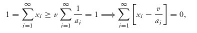
which means it must be true, since each term is nonnegative, xi = ![]() , i = 1, 2, …. Similarly, X* = Y*, and the components of both optimal strategies are
, i = 1, 2, …. Similarly, X* = Y*, and the components of both optimal strategies are ![]() , i = 1, 2, ….
, i = 1, 2, ….
1.39.c Just as in the second part, we have for any integer n > 1, aj xj ≥ v, which implies
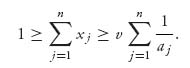
Then
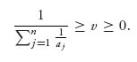
Sending n → ∞ on the left side and using the fact ![]() = ∞, we get v = 0. Note that we know ahead of time that v ≥ 0 since
= ∞, we get v = 0. Note that we know ahead of time that v ≥ 0 since
![]()
Let X = (x1, x2, …) be any mixed strategy for player I. Then, it is always true that E(X, j) = xjaj ≥ v = 0 for any column j. By Theorem 1.3.8 this says that X is optimal for player I. On the other hand, if Y* is optimal for player II, then E(i, Y*) = ai yi ≤ v = 0, i = 1, 2, … . Since ai > 0, this implies yi = 0 for every i = 1, 2, …. But then Y = (0, 0, …) is not a strategy and we conclude player II does not have an optimal strategy. Since the space of strategies in an infinite sequence space is not closed and bounded, we are not guaranteed that an optimal mixed strategy exists by the minimax theorem.
1.41 Using Problem 1.40 we have
Now, if (X*, Y*) is a saddle then v = E(X*, Y*) and
But we have seen that the two ends of this long inequality are the same. We conclude that
![]()
Conversely, if max1 ≤ i ≤ nE(i, Y*) = min1 ≤ j ≤ m E(X*, j) = a, then we have the inequalities
![]()
This immediately implies that (X*, Y*) is a saddle and a = E(X*, Y*) = value of the game.
1.43.a We will use the graphical method. The graph is
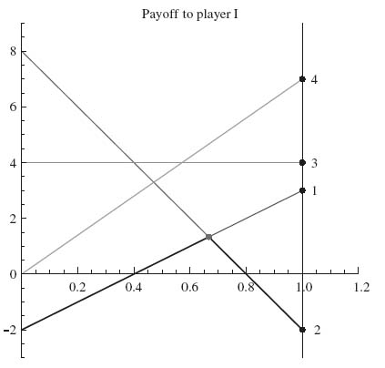
The figure indicates that the two lines determining the optimal strategies will cross where − 2x + 3(1 − x) = 8x + (− 2)(1 − x). This tells us that x* = ![]() and then v = − 2
and then v = − 2 ![]() + 3 (1 −
+ 3 (1 − ![]() ) =
) = ![]() . We have X* = (
. We have X* = (![]() ,
, ![]() ).
).
Next, since the two lines giving the optimal X* come from columns 1 and 2, we may drop the remaining columns and solve for Y* using the matrix ![]() The two lines for player II cross where 3y − 2(1 − y) = − 2 y + 8(1 − y), or y* =
The two lines for player II cross where 3y − 2(1 − y) = − 2 y + 8(1 − y), or y* = ![]() . Thus, Y* = (
. Thus, Y* = (![]() ,
, ![]() , 0, 0).
, 0, 0).
1.43.b The best response for player I to Y = (![]() ,
, ![]() ,
, ![]() ,
, ![]() ) is X = (0, 1). The reason is that if we look at the payoff for X = (x, 1 − x), we get
) is X = (0, 1). The reason is that if we look at the payoff for X = (x, 1 − x), we get
![]()
The maximum of this over 0 ≤ x ≤ 1 occurs when x = 0, which means the best response strategy for player I is X* = (0, 1), with expected payoff 4.
1.43.c Player I’s best response is X* = (0, 1), which means always play row II. Player II’s best response to that is always play column 1, Y* = (1, 0, 0, 0), resulting in a payoff to player I of − 2.
1.45.a The matrix is
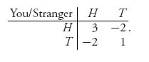
The saddle point is X* = (![]() ,
, ![]() ) = Y*. This is obtained from solving 3x − 2(1 − x) = − 2 x + (1 − x), and 3y − 2(1 − y) = − 2y + (1 − y). The value of this game is v = −
) = Y*. This is obtained from solving 3x − 2(1 − x) = − 2 x + (1 − x), and 3y − 2(1 − y) = − 2y + (1 − y). The value of this game is v = − ![]() , so this is definitely a game you should not play.
, so this is definitely a game you should not play.
1.45.b If the stranger plays the strategy ![]() = (
= (![]() ,
, ![]() ), then your best response strategy is
), then your best response strategy is ![]() = (0, 1), which means you will call Tails all the time. The reason is
= (0, 1), which means you will call Tails all the time. The reason is
which is maximised at x = 0. This results in an expected payoff to you of zero. ![]() is not a winning strategy for the stranger.
is not a winning strategy for the stranger.
1.47.a We can find the first derivatives and set to zero:
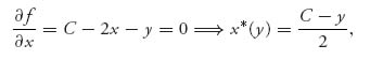
and
These are the best responses since the second partials fxx = gyy = − 2 > 0.
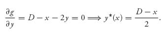
1.47.b Best responses are x = ![]() , y =
, y = ![]() , which can be solved to give x* =
, which can be solved to give x* = ![]() , y* =
, y* = ![]() .
.
Next,
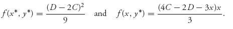
The maximum of f(x, y*) is ![]() , achieved at x =
, achieved at x = ![]() , which means it is true that f(x* y*) ≥ f(x, y*) for all x.
, which means it is true that f(x* y*) ≥ f(x, y*) for all x.
Solutions for Chapter 2
2.1 If we use the 2 × 2 formulas, we get det (A) = − 80, A* =  , so
, so
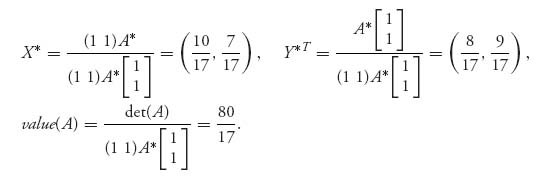
If we use the graphical method, the lines cross where x + 10(1 − x) = 8x ![]() x =
x = ![]() . The rest also checks.
. The rest also checks.
2.3 The new matrix is A = ![]() and the optimal strategies using the formulas become
and the optimal strategies using the formulas become
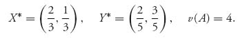
The defense will guard against the pass more.
2.5 Since there is no pure saddle, the optimal strategies are completely mixed. Then, Theorem 1.3.8 tells us for X* = (x, 1 − x),
![]()
which gives x = x* = ![]() . Then
. Then
Since A* =  ,
,

the formulas match.
The rest of the steps are similar to find Y* and v(A).
2.7 One possible example is A = ![]() , which obviously has a saddle at payoff 8, so that the actual optimal strategies are X* = (1, 0), Y* = (1, 0), v(A) = 8. However, if we simply apply the formulas, we get the nonoptimal alleged solution X* = (
, which obviously has a saddle at payoff 8, so that the actual optimal strategies are X* = (1, 0), Y* = (1, 0), v(A) = 8. However, if we simply apply the formulas, we get the nonoptimal alleged solution X* = (![]() ,
, ![]() ), Y* = (
), Y* = (![]() , −
, − ![]() ), which is completely incorrect.
), which is completely incorrect.
2.9 If we calculate f(k) = ![]() , we get f(1) = 4.5, f(2) = 5.90, f(3) = 5.94, and f(4) = 2.46. This gives us k* = 3. Then we calculate xi =
, we get f(1) = 4.5, f(2) = 5.90, f(3) = 5.94, and f(4) = 2.46. This gives us k* = 3. Then we calculate xi = ![]() and get
and get
and v(A) = ![]() = 5.943. Finally, to calculate Y*, we have
= 5.943. Finally, to calculate Y*, we have
This results in Y* = (0.6792, 0.30188, 0.01886, 0). Thus player I will attack target 3 about 40% of the time, while player II will defend target 3 with probability of only about 2%.
2.11 (a) The matrix has a saddle at row 1, column 2; formulas do not apply.
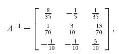
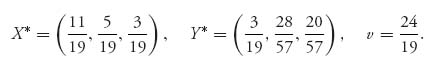
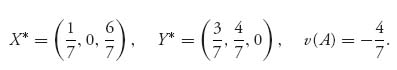
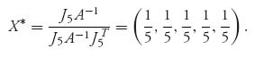
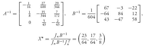
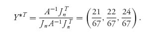
(b) The inverse of A is
The formulas then give X* = (![]() , 0,
, 0, ![]() ), Y* = (
), Y* = (![]() ,
, ![]() ,
, ![]() ) and v =
) and v = ![]() . There is another optimal Y* = (
. There is another optimal Y* = (![]() , 0,
, 0, ![]() ), which we can find by noting that the second column is dominated by a convex combination of the first and third columns (with λ =
), which we can find by noting that the second column is dominated by a convex combination of the first and third columns (with λ = ![]() ). This optimal strategy for player II is not obtained using the formulas. It is in fact optimal since
). This optimal strategy for player II is not obtained using the formulas. It is in fact optimal since
Since E(2, Y) = 2 < v(A), we know that the second component of an optimal strategy for player I must have x2 = 0.
(c) Since
the formulas give the optimal strategies
(d) The matrix has the last column dominated by column 1. Then player I has row 2 dominated by column 1. The resulting matrix is ![]() . This game can be solved with 2 × 2 formulas or graphically. The solution for the original game is then
. This game can be solved with 2 × 2 formulas or graphically. The solution for the original game is then
2.13 Use the definition of value and strategy to see that
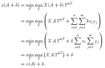
We also see that X, (A + b), YT = X A YT + b.
If (X* Y*) is a saddle for A, then
![]()
and
![]()
for any X, Y. Together this says that X*, Y* is also a saddle for A + b. The converse is similar.
2.15 By the invertible matrix theorem we have
Using the formulas we also have v(A) = 13 and Y* = X*. This leads us to suspect that each row and column, in the general case, is played with probability ![]() .
.
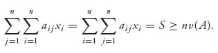
Now, let S denote the common sum of the rows and columns in an n × n magic square. For any optimal strategy X for player I and Y for player II, we must have
![]()
Since E(X, j) = ![]() aijxi ≥ v, adding for j = 1, 2, …, n, we get
aijxi ≥ v, adding for j = 1, 2, …, n, we get
Similarly, since E(i, Y) = ![]() aijyj ≤ v, adding for i = 1, 2, …, n, we get
aijyj ≤ v, adding for i = 1, 2, …, n, we get
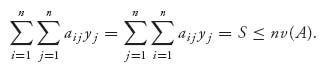
Putting them together, we have v(A) = ![]() .
.
Finally, we need to verify that X* = Y* = (![]() , …,
, …, ![]() ) is optimal. That follows immediately from the fact that
) is optimal. That follows immediately from the fact that
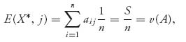
and similarly E(i, Y*) = v(A), i = 1, 2, …, n. We conclude using Theorem 1.3.8.
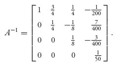
2.17 Since det A = ![]() =
= ![]() > 0, the matrix has an inverse. The inverse matrix is
> 0, the matrix has an inverse. The inverse matrix is
Then, setting q = ![]()
![]() we have
we have
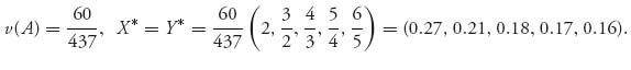
If n = 5, we have q = ![]() , so
, so
Note that you search with decreasing probabilities as the box number increases.
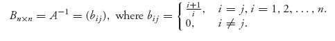
2.19.a The matrix has an inverse if det (A) ≠ 0. Since det (A) = a11a22 · · · ann, no diagonal entries may be zero.
2.19.b The inverse matrix is
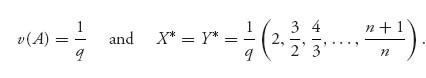
Then, we have
2.21 This is an invertible matrix with inverse
We may use the formulas to get (A) = ![]() , X* = Y* = (
, X* = Y* = (![]() ,
, ![]() ,
, ![]() ), and the cat and rat play each of the rows and columns of the reduced game with probability
), and the cat and rat play each of the rows and columns of the reduced game with probability ![]() . This corresponds to dcbi, djke, ekjd for the cat, each with probability
. This corresponds to dcbi, djke, ekjd for the cat, each with probability ![]() , and abcj, aike, hlia each with probability
, and abcj, aike, hlia each with probability ![]() for the rat. Equivalent paths exist for eliminated rows and columns.
for the rat. Equivalent paths exist for eliminated rows and columns.
2.23 The duelists shoot at 10, 6, or 2 paces with accuracies 0.2, 0.4, 1.0, respectively. The accuracies are the same for both players. The game matrix becomes
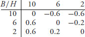
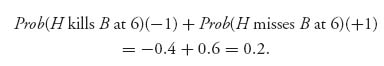
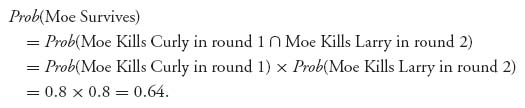
For example, if Burr decides to fire at 10 paces, and Hamilton fires at 10 as well, then the expected payoff to Burr is zero since the duelists have the same accuracies and payoffs (it’s a draw if they fire at the same time). If Burr decides to fire at 10 paces and Hamilton decides to not fire, then the outcome depends only on whether or not Burr kills Hamilton at 10. If Burr misses, he dies. The expected payoff to Burr is
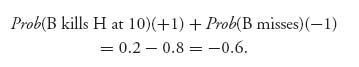
Similarly, Burr fires at 2 paces and Hamilton fires at 6 paces, then Hamilton’s survival depends on whether or not he missed at 6. The expected payoff to Burr is
Calculating the lower value we see that v− = 0 and the upper value is v+ = 0, both of which are achieved at row 3, column 3. We have a pure saddle point and both players should wait until 2 paces to shoot. Makes perfect sense that a duelist would not risk missing.
2.25 The matrix B is given by
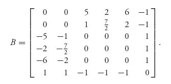
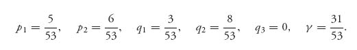
Now we use the method of symmetry to solve the game with matrix B. Obviously, v(B) = 0, and if we let P = (p1, …, p6) denote the optimal strategy for player I, we have
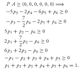
This system of inequalities has one and only one solution given by
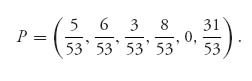
As far as the solution of the game with matrix B goes, we have v(B) = 0, and P is the optimal strategy for both players I and II.
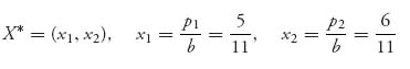
Now to find the solution of the original game, we have (now with a new meaning for the symbols pi) n = 2, m = 3 and
Then b = p1 + p2 = ![]() , b = q1 + q2 + q3 =
, b = q1 + q2 + q3 = ![]() =
= ![]() . Now define the strategy for the original game with A,
. Now define the strategy for the original game with A,
and
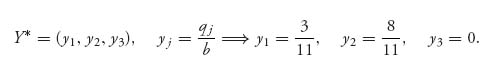
Finally, v(A) = ![]() =
= ![]() =
= ![]() .
.
The problem is making the statement that this is indeed the solution of our original game. We verify that by calculating using the original matrix A,
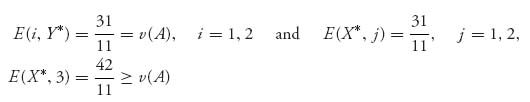
By Theorem 1.3.8 we conclude that X*, Y* is optimal and v(A) = ![]() .
.
2.27 For method 1 the LP problem for each player is:
| Player I Min z1 = p1 + p2 + p3 + p4 4 p1 + 9 p2 + 10 p3 + 8 p4 ≥ 1 9 p1 + 4 p2 + p3 + 2 p4 ≥ 1 9 p1 + p2 + 5 p3 + 9 p4 ≥ 1 10 p1 + 8 p2 + 10 p3 + 10 p4 ≥ 1 7 p1 + 10 p2 + 5 p3 + 3 p4 ≥ 1 pi ≥ 0 . | Player II Max z2 = q1 + q2 + q3 + q4 + q5 4 q1 + 9 q2 + 9 q3 + 10 q4 + 7 q5 ≤ 1 9 q1 + 4 q2 + q3 + 8 q4 + 10 q5 ≤ 1 10 q1 + q2 + 5 q3 + 10 q4 + 5 q5 ≤ 1 8 q1 + 2 q2 + 9 q3 + 10 q4 + 3 q5 ≤ 1 qj ≥ 0. |
For method 2, the LP problems are as follows:
| Player I Max v − 2 x1 + 3 x2 + 4 x3 + 2 x4 ≥ v 3 x1 − 2 x2 − 5 x3 − 4 x4 ≥ v 3 x1 − 5 x2 − x3 + 3 x4 ≥ v 4 x1 + 2 x2 + 4 x3 + 4 x4 ≥ v x1 + 4 x2 − x3 − 3 x4 ≥ v xi ≥ 0 ∑ xi = 1. | Player II Min v − 2 y1 + 3 y2 + 3 y3 + 4 y4 + y5 ≤ v 3 y1 − 2 y2 − 5 y3 + 2 y4 + 4 y5 ≤ v 4 y1-5 y2 − y3 + 4 y4 − y5 ≤ v 2 y1 − 4 y2 + 3 y3 + 4 y4 − 3 y5 ≤ v yj ≥ 0 ∑ yj = 1. |
Both methods result in the solution
![]()
2.29 We cannot use the invertible matrix theorem but we can use linear programming. To set this up we have, in Maple,
 > with(LinearAlgebra):with(simplex):
 > A: = Matrix([[1, -4, 6, -2], [-8, 7, 2, 1], [11, -1, 3, -3]]);
 > X: = Vector(3, symbol = x);
 > B: = Transpose(X).A;
 > cnstx: = seq(B[j] > = v, j = 1..4), seq(x[i] > = 0, i = 1..3),
          add(x[i], i = 1..3) = 1;
 > maximize(v, cnstx);
This results in X* = (0, ![]() and v(A) = −
and v(A) = − ![]() . It looks like John should not bother with State 1, and spend most of his time in State 2. For Dick, the problem is
. It looks like John should not bother with State 1, and spend most of his time in State 2. For Dick, the problem is
 > Y: = < y[1], y[2], y[3], y[4] > ;
 > B: = A.Y;
 > cnsty: = seq(B[j] < = w, j = 1..3), seq(y[j] > = 0, j = 1..4),
          add(y[j], j = 1..4) = 1;
 > minimize(w, cnsty);
The result is Y* = (![]() , 0, 0,
, 0, 0, ![]() ). Dick should skip States 2 and 3 and put everything into States 1 and 4. John should think about raising more money to be competitive in State 4, otherwise, John suffers a net loss of −
). Dick should skip States 2 and 3 and put everything into States 1 and 4. John should think about raising more money to be competitive in State 4, otherwise, John suffers a net loss of − ![]() .
.
2.31 Each player has eight possible strategies but many of them are dominated. The reduced matrix is
Referring to the Figure 1.1 we have the strategies for rat: 1 = hgf, 2 = hlk, 3 = abc, and for cat, A = djk, B = ekj.
The solution is the cat should take small loops and the rat should stay along the edges of the maze. X* = (![]() ,
, ![]() ), Y* = (
), Y* = (![]() , 0,
, 0, ![]() ) and v =
) and v = ![]() .
.
2.33 LUC is the row player and UIC the column player. The strategies for LUC are AA, AB, BA, BB. UIC has strategies XX, XY, …, indicated in the table
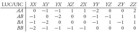
The numbers in the table are obtained from the rules of the game. For example, if LUC plays AB and UIC plays XY, then the expected payoff to LUC on each match is zero and hence on both matches it is zero.
Solving this game with Maple/Mathematica/Gambit, we get the saddle point
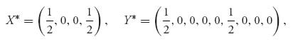
so LUC should play AA and BB with equal probability, and UIC should play XX, YY with equal probability. Z is going to sit out. The value of the game is v = −1, and it looks like LUC loses the tournament.
2.35 The game matrix is
To use Maple to get these matrices:
Accuracy functions:
 > p1: = x- > piecewise(x = 0, .2, x = .2, .4, x = .4, .4, x = .6, .4, x = .8, 1);
 > p2: = x- > piecewise(x = 0, 0.6, x = .2, .8, x = .4, .8, x = .6, .8, x = .8, 1);
Payoff function
 > u1: = (x, y)- >
      piecewise(x < y, 1*p1(x) +
              (-1)*(1-p1(x))*p2(y) +
              (0)*(1-p1(x))*(1-p2(y)),
      x > y, (-1)*p2(y) + (1)*(1-p2(y))*p2(x) + 0*(1-p2(y))*(1-p1(x)),
      x = y, 0*p1(x)*p2(x) + (1)*p1(x)*(1-p2(x)) + (-1)*(1-p1(x))*p2(x)
      + 0*(1-p1(x))*(1-p2(x)));
 > with(LinearAlgebra):
 > A: = Matrix([[u1(0, 0), u1(0, .4), u1(0, .8)],
          [u1(.4, 0), u1(.4, .4), u1(.4, .8)],
          [u1(.8, 0), u1(.8, .4), u1(.8, .8)]]);
The solution of this game is
![]()
2.37 The matrix is
Then, X* =, (0.43, 0.086.0.152, 0.326, 0, 0, 0), Y* = (0.043, 0.217, 0.413, 0.326, 0, 0, 0), v = 2.02174. This says 43% of the time farmer I should concede nothing, while farmer II should concede 2 about 41% of the time. Since the value to farmer I is about 2, farmer II will get about 4 yards. The rules definitely favor farmer II.
In the second case, in which the judge awards 3 yards to each farmer if they make equal concessions, each farmer should concede 2 yards and the value of the game is 3. Observe that the only difference between this game's matrix and the previous game is that the matrix has 3 on the main diagonal. This game, however, has a pure saddle point.
2.39 The solution is X = (![]() ,
, ![]() ), Y = (1, 0, 0...), v = a. If you graph the lines for player I versus the columns ending at column n, you will see that the lines that determine the optimal strategy for I will correspond to column 1 and the column with (2a, 1/n), or (1/n, 2a). This gives x* =
), Y = (1, 0, 0...), v = a. If you graph the lines for player I versus the columns ending at column n, you will see that the lines that determine the optimal strategy for I will correspond to column 1 and the column with (2a, 1/n), or (1/n, 2a). This gives x* = ![]() . Letting n→ ∞ gives x* =
. Letting n→ ∞ gives x* = ![]() . For player II, you can see from the graph that the last column and the first column are the only ones being used, which leads to the matrix for player II for a fixed n of
. For player II, you can see from the graph that the last column and the first column are the only ones being used, which leads to the matrix for player II for a fixed n of ![]() . For all large enough n, so that 2a > 1/n, we have a saddle point at row 1, column 1, independent of n, which means Y* = (1, 0, 0, …).
. For all large enough n, so that 2a > 1/n, we have a saddle point at row 1, column 1, independent of n, which means Y* = (1, 0, 0, …).
For example, if we take a = ![]() , and truncate it at column 5, we get the matrix
, and truncate it at column 5, we get the matrix
and the graph is shown.
The solution of this game is
![]()
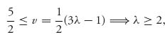
2.41.a First, we have to make sure that X* is a legitimate strategy. The components add up to 1 and each component is ≥ 0 as long as 0 ≤ λ ≤ 1, so it is legitimate.
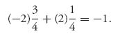
Next, we calculate E(X*, Y*) = X*A, Y*T = ![]() (3λ −1) for any λ. Thus, we must have v(A) =
(3λ −1) for any λ. Thus, we must have v(A) = ![]() (3 λ −1) and v(A) = −
(3 λ −1) and v(A) = − ![]() , if λ = 0.
, if λ = 0.
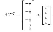
Now, we have to check that (X*, Y*) is a saddle point and v(A) is really the value. For that, we check
![]()
The last inequalities are not true (unless λ = 0), since
![]()
Finally, we check
The last inequalities are not all true because − ![]() ≤ −
≤ − ![]() +
+ ![]() λ = v, but
λ = v, but
and that contradicts 0 ≤ λ ≤ 1. Thus, everything falls apart.
2.41.b First note that the first row can be dropped because of strict dominance. Then we are left with the matrix 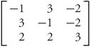
The solution of the game is X* = (0, 0, 0, 1), Y* = (![]() ,
, ![]() , 0), v(A) = 2.
, 0), v(A) = 2.
2.43.a The game matrix is
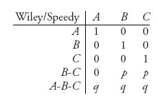
This reflects the rules that if Wiley waits at the right exit, Speedy will be caught. If Wiley waits between B and C, Speedy is caught with probability p if he exits from B or C, but he gets away if he comes out of A. If Wiley overlooks all three exits he has equal probability q of catching Speedy no matter what Speedy chooses.
2.43.b If any convex combination of the first 3 rows dominates row 4, we can drop row 4. Dominance requires then that we must have numbers λ1, λ2, λ3, such that λ1 > 0, λ2 > p, λ3 > p, where λ1 + λ2 + λ3 = 1, λi ≥ 0. Adding gives 1 = λ1 + λ2 + λ3 ≥ 2p ![]() p <
p < ![]() for strict domination. Similarly, for row 5, strict domination would imply λ1 + λ2 + λ3 > 3 q
for strict domination. Similarly, for row 5, strict domination would imply λ1 + λ2 + λ3 > 3 q ![]() q <
q < ![]() . Thus, if p <
. Thus, if p < ![]() or q <
or q < ![]() , Wiley should pick an exit and wait there.
, Wiley should pick an exit and wait there.
2.43.c The linear programming setup for this problem is
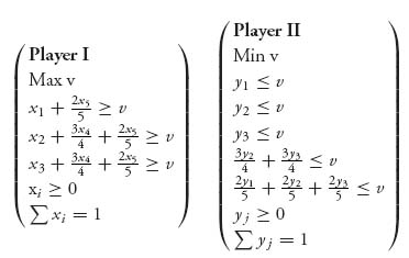
The solution of the game by linear programming is X* = (![]() , 0, 0,
, 0, 0, ![]() , 0), Y* = (
, 0), Y* = (![]() ,
, ![]() ,
, ![]() ), and v(A) =
), and v(A) = ![]() . Since B and C are symmetric, another possible Y* = (
. Since B and C are symmetric, another possible Y* = (![]() ,
, ![]() ,
, ![]() ). A little less than half the time Wiley should wait outside A, and the rest of the time he should overlook all three exits. Speedy should exit from A with probability
). A little less than half the time Wiley should wait outside A, and the rest of the time he should overlook all three exits. Speedy should exit from A with probability ![]() and either B or C with probability
and either B or C with probability ![]() .
.
2.45 Sonny has two strategies: (1) Brooklyn, (2) Queens. Barzini also has two strategies: (1) Brooklyn, (2) Queens. If Sonny heads for Brooklyn and Barzini also heads for Brooklyn, Sonny’s expected payoff is
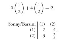
This game is easily solved using 2x + 3(1 − x) = 4x + ![]() (1 − x)
(1 − x) ![]() x =
x = ![]() , and 2y + 4(1 − y) = 3y +
, and 2y + 4(1 − y) = 3y + ![]() (1 − y), which gives y =
(1 − y), which gives y = ![]() . The optimal strategies are
. The optimal strategies are
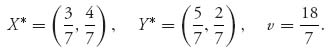
Sonny should head for Queens with probability ![]() , and Barzini should head for Brooklyn with probability
, and Barzini should head for Brooklyn with probability ![]() . On average, Sonny rescues between 2 and 3 capos.
. On average, Sonny rescues between 2 and 3 capos.
2.47.a X* = (![]() ,
, ![]() ), Y* = (
), Y* = (![]() , 0, 0,
, 0, 0, ![]() , 0).
, 0).
2.47.b X* = (![]() ,
, ![]() ,
, ![]() , 0), Y* = (
, 0), Y* = (![]() ,
, ![]() ,
, ![]() , 0), v =
, 0), v = ![]() .
.
2.47.c X* = (![]() ), Y* = (
), Y* = (![]() , 0), v =
, 0), v = ![]() .
.
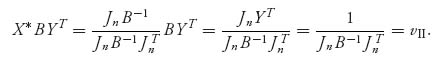
2.49 In order for (X*, Y*) to be a saddle point and v to be the value, it is necessary and sufficient that E(X*j) ≥ v, for all j = 1, 2, …, m and E(i, Y*) ≤ v for all i = 1, 2, …, n.
2.51 E(k, Y*) = v(A). If xk = 0, E(k, Y*) ≤ v(A).
2.53
2.55
![]()
for i = 1, 2, …, n, j = 1, 2, …, m.
2.57 True.
2.59 xi = 0.
2.61 True.
2.63 False. Only if you know x1 = 0 for every optimal strategy for player I.
2.65 X* = (0, 1, 0), Y* = (0, 0, 1, 0).
2.67 False. There’s more to it than that.
2.69 True! This is a point of logic. Since any skew symmetric game must have v(A) = 0, the sentence has a false premise. A false premise always implies anything, even something that is false on it’s own (since -Y* can’t even be a strategy).
Solutions for Chapter 3
3.1 Use the definitions. For example, if X*, Y* is a Nash equilibrium, then X*AY*T ≥ XAY*T, ∀ X, and X*(− A)Y*T ≥ X*(− A)YT, ∀ Y. Then
![]()
3.3.a The two pure Nash equilibria are at (Turn, Straight) and (Straight, Turn).
3.3.b To verify that X* = (![]() ), Y* = (
), Y* = (![]() ) is a Nash equilibrium we need to show that
) is a Nash equilibrium we need to show that
![]()
for all strategies X, Y. Calculating the payoffs, we get
for any X = (x, 1 − x), 0 ≤ x ≤ 1. Similarly,
Since EI(X*, Y*) = EII (X*, Y*) = −![]() , we have shown (X*, Y*) is a Nash equilibrium.
, we have shown (X*, Y*) is a Nash equilibrium.
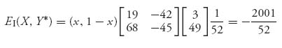
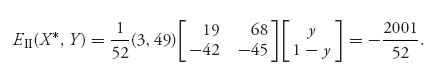
3.3.c For player I, A = ![]() . Then v(A) = − 42 and that is the safety level for I. The maxmin strategy for player I is X = (1, 0). For player II, BT =
. Then v(A) = − 42 and that is the safety level for I. The maxmin strategy for player I is X = (1, 0). For player II, BT = ![]() , so the safety level for II is also v(BT) = − 42. The maxmin strategy for player II is XBT = (1, 0).
, so the safety level for II is also v(BT) = − 42. The maxmin strategy for player II is XBT = (1, 0).
3.5.a Weak dominance by row 1 and then strict dominance by column 2 gives the Nash equilibrium at (5, 1).
3.5.b Player II drops the third column by strict dominance. This gives the matrix
Then we have two pure Nash equilibria at (10, 1) and (5, 1).
3.7 There is one pure Nash at (Low, Low). Both airlines should set their fares low.
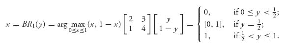
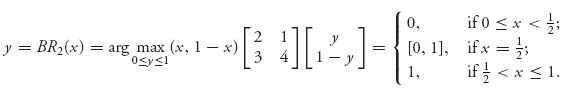
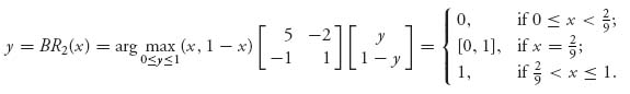
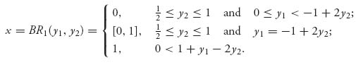
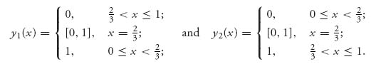
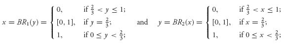
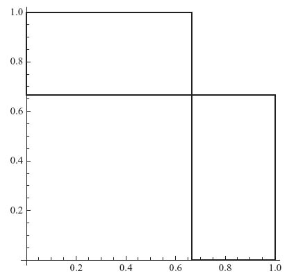
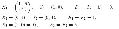
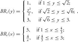
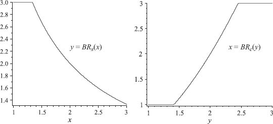
3.9.a Graph x = BR1 (y) and y = BR2(x) on the same set of axes. Where the graphs intersect is the Nash equilibrium (they could intersect at more than one point). The unique Nash equilibrium is X* = (![]() ,
, ![]() ), Y* = (
), Y* = (![]() ,
, ![]() ).
).
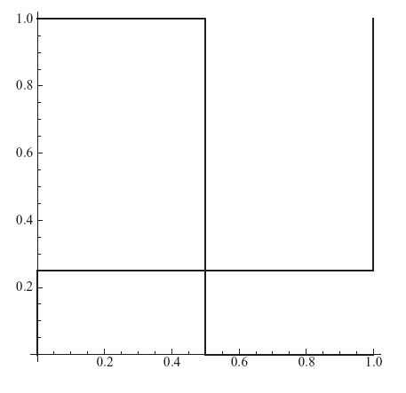
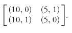
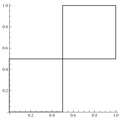
3.9.b Here is a plot of the four lines bounding the best response sets:
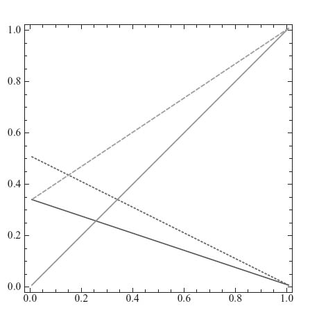
The intersection of the two sets constitutes all the Nash equilibria. Mathematica characterizes the intersection as
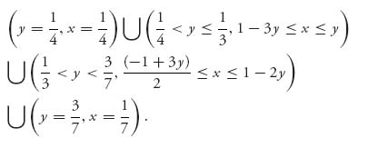
You can see from the figure that there are lots of Nash equilibria. For example x* = ![]() , y* =
, y* = ![]() , is one.
, is one.
3.11 We calculate the best response functions
and
Graphing these two functions shows that they intersect at (0, 0), (![]() ,
, ![]() ), (1, 1):
), (1, 1):
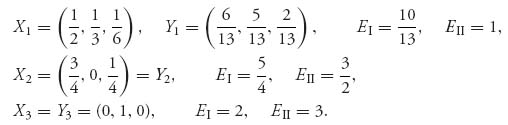
The Nash equilibria are X1 = (![]() ,
, ![]() ), Y1 = (
), Y1 = (![]() ,
, ![]() ), X2 = (0, 1) = Y2, X3 = (1, 0) = Y3.
), X2 = (0, 1) = Y2, X3 = (1, 0) = Y3.
3.13 To find the best response functions calculate
and
Here’s the figure:
The only Nash is X = (![]() ,
, ![]() ), Y = (
), Y = (![]() ), with payoffs −
), with payoffs − ![]() ,
, ![]() . The rational reaction sets intersect at only this Nash.
. The rational reaction sets intersect at only this Nash.
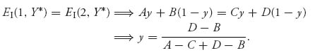
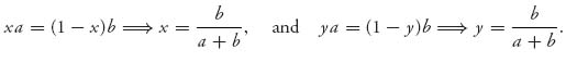
3.15.a Let X* = (x, 1 − x). By equality of payoffs, assuming both columns are played with positive probability, we get the equations
Then X* = (![]() ). In order for this to work, X* must be a legitimate strategy with positive components.
). In order for this to work, X* must be a legitimate strategy with positive components.
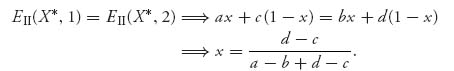
3.15.b Let Y* = (y, 1 − y). Assuming both rows are played with positive probability,
This requires that A-C + D-B ≠ 0 and D ≠ B. Then Y* = (![]() ) and the components must be positive.
) and the components must be positive.
3.17 We need to check that EI(X*, Y*) ≥ EI(i, Y*), i = 1, 2, 3, and EII (X*, Y*) ≥ EII(X*j), j = 1, 2, 3. Calculating, we get
Each of these numbers is ≤ ![]() . Next,
. Next,
![]()
Each of these are actually equal to ![]() . We conclude that X*, Y* is indeed a Nash equilibrium.
. We conclude that X*, Y* is indeed a Nash equilibrium.
3.19.a The pure strategies for each son is the share of the estate to claim. The matrix is
There are three pure Nash equilibria: (1) row 1, column 3, (2) row 2, column 2, and (3) row 3, column 1.
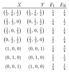
3.19.b The table contains the pure and mixed Nash points as well as the payoffs.
To use the equality of payoffs theorem to find these you must consider all possibilities in which at least two rows (or columns) are played with positive probability. For example, suppose that columns 2 and 3 are used by player II with positive probability. Equality of payoffs then tells us
![]()
Hence, X = (x1, 0.5 x1, 1-1.5 x1) is a solution as long as 0 > x1 < ![]() .
.
If x1 = 0, we get X = (0, 0, 1), which is part of a pure Nash but is not obtained from equality of payoffs. If x1 = ![]() then X = (
then X = (![]() ,
, ![]() , 0). By equality of payoffs we then obtain
, 0). By equality of payoffs we then obtain
Then, Y = (y1, ![]() − y1,
− y1, ![]() ) is the solution if 0 ≤ y1 <
) is the solution if 0 ≤ y1 < ![]() . Observe that y1 =
. Observe that y1 = ![]() is not consistent with our original assumption that y2 > 0, y3 > 0, but y1 = 0 is. In that case, Y = (0,
is not consistent with our original assumption that y2 > 0, y3 > 0, but y1 = 0 is. In that case, Y = (0, ![]() ,
, ![]() ) and we have the Nash equilibrium X = (
) and we have the Nash equilibrium X = (![]() ,
, ![]() , 0), Y = (0,
, 0), Y = (0, ![]() ,
, ![]() ). Any of the remaining Nash equilibria in the tables are obtained similarly.
). Any of the remaining Nash equilibria in the tables are obtained similarly.
If we assume Y = (y1, y2, y3) is part of a mixed Nash with yj > 0, j = 1, 2, 3, then equality of payoffs gives the equations
The first and fourth equations give vI = 0.25. Then the third equation gives x1 = ![]() , then x2 =
, then x2 = ![]() , and finally x3 =
, and finally x3 = ![]() . Since X = (
. Since X = (![]() ,
, ![]() ,
, ![]() ), we then use equality of payoffs to find Y. The equations are as follows:
), we then use equality of payoffs to find Y. The equations are as follows:
This has the same solution as before Y = X, vI = vII = 0.25, and this is consistent with our original assumption that all components of Y are positive.
3.21 We find the best response functions. For the government,
Similarly,
The Nash equilibrium is X = (![]() ,
, ![]() ), Y = (
), Y = (![]() ,
, ![]() ) with payoffs EI = −
) with payoffs EI = − ![]() , EII =
, EII = ![]() . The government should aid half the paupers, but 80% of paupers should be bums (or the government predicts that 80% of welfare recipients will not look for work). The rational reaction sets intersect only at the mixed Nash point.
. The government should aid half the paupers, but 80% of paupers should be bums (or the government predicts that 80% of welfare recipients will not look for work). The rational reaction sets intersect only at the mixed Nash point.
3.23 The system is 0 = 4y1 − y2, y1 + y2 = 1, which gives y1 = ![]() , y2 =
, y2 = ![]() .
.
3.25.a Assuming that the formulas actually give strategies we will show that the strategies are a Nash equilibrium. We have
and for any strategy X ![]() Sn,
Sn,
Similarly,
and for any Y ![]() Sn,
Sn,
3.25.b We have
and
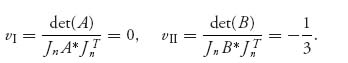
These are both legitimate strategies. Finally, vI = ![]() , vII =
, vII = ![]() .
.
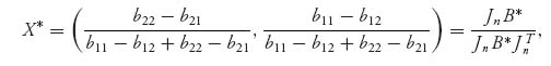
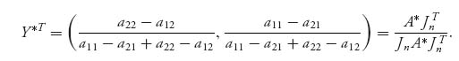
3.25.c Set A* = 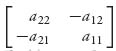 and B* =
 ![]() . Then, from the formulas derived in Problem 3.15 we have, assuming both rows and columns are played with positive probability,
. Then, from the formulas derived in Problem 3.15 we have, assuming both rows and columns are played with positive probability,
and
(X*, Y*) is a Nash equilibrium if they are strategies, and then
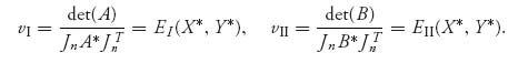
Of course, if A or B does not have an inverse, then det (A) = 0 or det (B) = 0.
For the game in (1), A* = ![]() and B* =
and B* = ![]() . We get
. We get
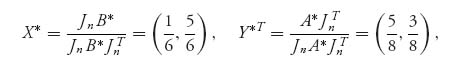
and
There are also two pure Nash equilibria, X1* = (0, 1), Y1* = (0, 1) and X2* = (1, 0), Y2* = (1, 0).
For the game in (2), A* = ![]() and B* =
and B* = ![]() . We get
. We get
and
In this part of the problem, A does not have an inverse and det (A) = 0. There are also two pure Nash equilibria, X1* = (0, 1), Y1* = (0, 1) and X2* = (1, 0), Y2* = (1, 0).
3.27 If ab < 0, there is exactly one strict Nash equilibrium: (i) a > 0, b < 0 ![]() the Nash point is X* = Y* = (1, 0); (ii) a < 0, b > 0
the Nash point is X* = Y* = (1, 0); (ii) a < 0, b > 0 ![]() the Nash point is X* = Y* = (0, 1). The rational reaction sets are simply the lines along the boundary of the square [0, 1] × [0, 1]: either x = 0, y = 0 or x = 1, y = 1.
the Nash point is X* = Y* = (0, 1). The rational reaction sets are simply the lines along the boundary of the square [0, 1] × [0, 1]: either x = 0, y = 0 or x = 1, y = 1.
If a > 0, b > 0, there are three Nash equilibria: X1 = Y1 = (1, 0), X2 = Y2 = (0, 1) and, the mixed Nash, X3 = Y3 = (![]() ). The mixed Nash is obtained from equality of payoffs:
). The mixed Nash is obtained from equality of payoffs:
If a < 0, b < 0, there are three Nash equilibria: X1 = (1, 0), Y1 = (0, 1), X2 = (0, 1), Y2 = (1, 0) and, the mixed Nash, X3 = Y3 = (![]() ). The rational reaction sets are piecewise linear lines as in previous figures which intersect at the Nash equilibria.
). The rational reaction sets are piecewise linear lines as in previous figures which intersect at the Nash equilibria.
3.29.a First we define f(x, y1, y2) = XAYT, where X = (x, 1 − x), Y = (y1, y2, 1 − y1 − y2). We calculate
![]()
and
Similarly,
![]()
and the maximum of g is achieved at (y1, y2), where
The best response set, BR2(x), for player II is the set of all pairs (y1(x), y2(x)).
This is obtained by hand or using the simple Mathematica commands:
![]()
3.29.b This is a little tricky because we don’t know which columns are used by player II with positive probability. However, if we note that column 3 is dominated by a convex combination of columns 1 and 2, we may drop column 3. Then the game is a 2× 2 game and
Then, for player II
The Nash equilibrium is X* = (![]() ,
, ![]() ), Y* = (
), Y* = (![]() ,
, ![]() , 0). Then y1 =
, 0). Then y1 = ![]() , y2 =
, y2 = ![]() , x =
, x = ![]() , and by definition
, and by definition ![]()
![]() BR1(
BR1(![]() ,
, ![]() ). Also, (
). Also, (![]() ,
, ![]() )
) ![]() BR2(
BR2(![]() ).
).
3.31 There are three Nash equilibria: X1 = (0, 1), Y1 = (0, 1); X2 = (1, 0), Y2 = (1, 0); X3 = (![]() ,
, ![]() ) = Y3 The last Nash gives payoffs (0, 0). The best response functions are as follows:
) = Y3 The last Nash gives payoffs (0, 0). The best response functions are as follows:
The Mathematica commands to solve this and all the 2 × 2 games are the following:
A = {{-1, 2}, {0, 0}}
f[x_, y_] = {x, 1 - x}.A.{y, 1 - y}
Maximize[{f[x, y], 0 < = x < = 1}, {x}]
B = {{-1, 0}, {2, 0}}
g[x_, y_] = {x, 1 - x}.B.{y, 1 - y}
Maximize[{g[x, y], 0 < = y < = 1}, {y}]
Show[{Graphics[Line[{{0, 1}, {0, 2/3}, {1, 2/3}, {1, 0}}]],
         Graphics[Line[{{0, 1}, {2/3, 1}, {2/3, 0}, {1, 0}}]]},
           Axes - > True]
The last command produces the graph:
Hawk–Dove best response sets
3.33.a First, note that there is no pure Nash equilibrium. We could use Problem 3.25 to solve this problem or do it directly by equality of payoffs. The equations to solve are as follows:
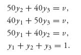
Adding the first three equations and using the fourth gives us v = 30. Then solving the first three equations gives Y* = (![]() ,
, ![]() ,
, ![]() ). Since the game is symmetric, X* = Y*. The expected payoff to each player is 30.
). Since the game is symmetric, X* = Y*. The expected payoff to each player is 30.
3.33.b If player II uses Y = (y1, y2, y3), then the expected payoff to player I is
![]()
The best response for player I will be to choose xi = 1 corresponding to the largest coefficient in EI. The only way to get a mixed strategy as a best response for player I is if the coefficients are all equal, and then they must all be 30, as we have seen. Thus, at least one coefficient must be greater than 30. Assume 50y2 + 40y3 > 30. Then, x1 = 1, x2 = x3 = 0 and player I’s expected payoff will be 50y2 + 40y3 > 30. Thus, no matter what, if player II does not use the mixed Nash, then player I’s expected payoff using the best response will be more than 30. This also applies for player II. Thus, if any player deviates from the Nash equilibrium, the best response gives a larger expected payoff to the other player.
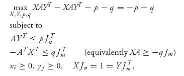
3.35 Since this is a 2 × 2 game, all we need to do is match up the coefficients in the constraints AYT ≤ pJ2T and XB ≤ q J2. A = ![]() , B =
, B = ![]() . Then use Maple/Mathematica to get X* = (0.7, 0.3), Y* = (0.6, 0.4), p = 62, q = 38.
. Then use Maple/Mathematica to get X* = (0.7, 0.3), Y* = (0.6, 0.4), p = 62, q = 38.
3.37 Take B = − A. The algorithm is then
where Jk = (1 1 1 · · · 1) is the 1 × k row vector consisting of all 1’s. In addition, p* = EI(X*, Y*) = X*AY*T, and q* = EII(X*, Y*) = − X*AY*T = − p*. You can see that this problem is the same as method 2 of linear programming for solving a game. Thus, Lemke–Howson reduces to method 2.
The Nash equilibrium found using Lemke–Howson is X* = (![]() ,
, ![]() , 0), Y* = (0,
, 0), Y* = (0, ![]() ,
, ![]() ), and the value of the game is v(A) =
), and the value of the game is v(A) = ![]() .
.
3.39 The Nash equilibria are as follows:
The corresponding respective payoffs are as follows:
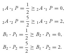
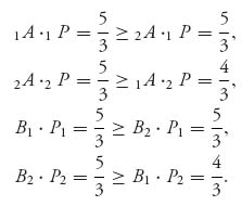
3.41 This is just rearranging the terms in the inequalities giving the definition of correlated equilibrium:
Using P we calculate the expected payoff for each player:
The payoff to player II is similar—just change the matrix.
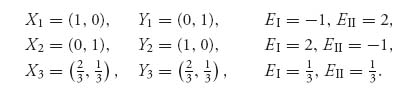
3.43 This chicken game has three Nash equilibria. There are two pure Nash equilibria at (5, 1), (1, 5). There is a mixed Nash equilibrium X* = Y* = (![]() ,
, ![]() ).
).
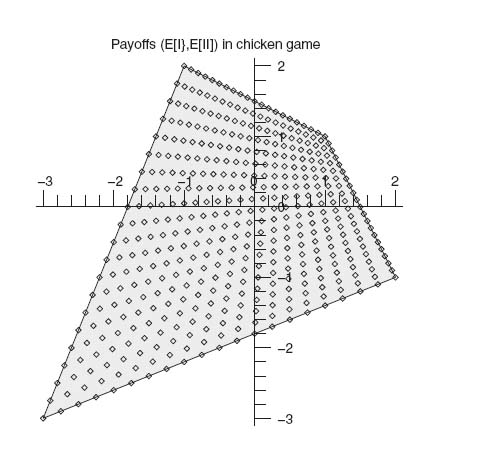
Now P1 and P2 correspond to the two pure Nash equilibria. Under P1 and P2, the social welfare is 6. Also P3 corresponds to the mixed Nash equilibrium with social welfare 5. Since P = X*TY* = (xiyj), if (X*, Y*) is a Nash equilibrium, then Pi, i = 1, 2, 3, is a correlated equilibrium.
Next consider P4. We have
Thus P4 is a correlated equilibrium. The social welfare under P4 is 6.
Finally consider P5. We have
Thus, P5 is also a correlated equilibrium. The social welfare under P5 is ![]() .
.
P5 is the correlated equilibrium that maximizes the social welfare. This comes from the solution of
Maximize[{Sum[Sum[(A[[i, j]] + B[[i, j]])Q[[i, j]], {j, 1, 2}], {i, 1, 2}],
A[[1]].Q[[1]] > = A[[2]].Q[[1]], A[[2]].Q[[2]] > = A[[1]].Q[[2]],
B[[All, 1]].Q[[All, 1]] > = B[[All, 2]].Q[[All, 1]],
B[[All, 2]].Q[[All, 2]] > = B[[All, 1]].Q[[All, 2]],
q11 + q12 + q21 + q22 = = 1,
q11 > = 0, q22 > = 0, q12 > = 0, q21 > = 0},
{q11, q12, q21, q22}]
3.45.a The Nash equilibria are as follows:
They are all Pareto-optimal because it is impossible for either player to improve their payoff without simultaneously decreasing the other player’s payoff, as you can see from the figure:
None of the Nash equilibria are payoff-dominant. The mixed Nash (X3, Y3) risk dominates the other two.
3.45.b The Nash equilibria are as follows:
(X3, Y3) is payoff-dominant and Pareto-optimal.
3.45.c
Clearly, X3, Y3 is payoff-dominant and Pareto-optimal. Neither (X1, Y1) nor (X2, Y2) are Pareto-optimal relative to the other Nash equilibria, but they each risk dominate (X3, Y3).
Solutions for Chapter 4
4.1 Player I has two pure strategies: 1 = take action 1 at node 1:1, and 2 = take action 2 at node 1:1. Player II has three pure strategies: 1 = take action 1 at information set 2:1, 2 = take action 2 at 2:1 and 3 = take action 3 at 2:1.
The game matrix is
There is a pure Nash at (4, 1).
4.3.a The extensive form along with the solution is shown in the figure:
Three-player game tree
The probability a player takes a branch is indicated below the branch.
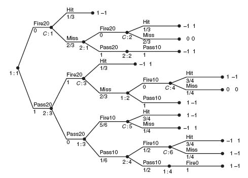
4.5.a The game tree follows the description of the problem in a straightforward way. It is considerably simplified if you use the fact that if a player fires the pie and misses, all the opponent has to do is wait until zero paces and winning is certain. Here is the tree.
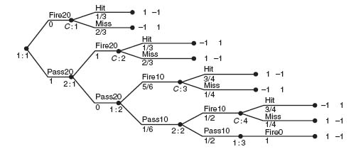
Aggie has three pure strategies:
(a1) Fire at 20 paces;
(a2) Pass at 20 paces; if Baggie passes at 20, fire at 10 paces;
(a3) Pass at 20 paces; if Baggie passes at 20, pass at 10 paces; if Baggie passes at 10, fire at 0 paces.
Baggie has three pure strategies:
(b1) If Aggie passes, fire at 20 paces;
(b2) If Aggie passes, pass at 20 paces; if Aggie passes at 10, fire at 10 paces;
(b3) If Aggie passes, pass at 20 paces; if Aggie passes at 10, pass at 10 paces.
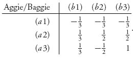
The game matrix is then
To see where the entries come from, consider (a1) versus (b1). Aggie is going to throw her pie and if Baggie doesn’t get hit, then Baggie will throw her pie. Aggie’s expected payoff will be
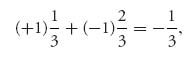
because Aggie hits Baggie with probability ![]() and gets + 1, but if she misses, then she is going to get a pie in the face.
and gets + 1, but if she misses, then she is going to get a pie in the face.
If Aggie plays (a2) and Baggie plays (b3), then Aggie will pass at 20 paces; Baggie will also pass at 20; then Aggie will fire at 10 paces. Aggies’ expected payoff is then
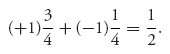
4.5.b The solution of the game can be obtained from the matrix using dominance. The saddle point is for Aggie to play (a2) and Baggie plays (b1). In words, Aggie will pass at 20 paces, Baggie will fire at 20 paces, with value v = ![]() to Aggie. Since Baggie moves second, her best strategy is to take her best shot as soon as she gets it.
to Aggie. Since Baggie moves second, her best strategy is to take her best shot as soon as she gets it.
Here is a slightly modified version of this game in which both players can miss their shot with a resulting score of 0. The value of the game is still ![]() to Aggie. It is still optimal for Aggie to pass at 20, and for Baggie to take her shot at 20. If Baggie misses, she is certain to get a pie in the face.
to Aggie. It is still optimal for Aggie to pass at 20, and for Baggie to take her shot at 20. If Baggie misses, she is certain to get a pie in the face.
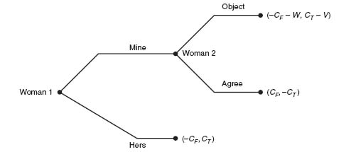
4.7 Assume first that woman 1 is the true mother. We look at the matrix for this game:
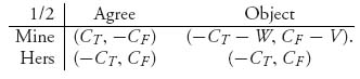
Since V > 2CF, there are two pure Nash equilibria: (1) at (CT, -CF) and (2) at (− CT, CF). If we consider the tree, we see that woman 2 will always Agree if woman 1 claims Mine. This eliminates the branch Object by woman 2. Next, since CT > -CT, woman 1 will always call Mine, and hence woman 1 will end up with the child. The Nash equilibrium (CT, − CF) is the equilibrium that will be played by backward induction. Note that we can’t obtain that conclusion just from the matrix.
Woman 1 the true mother
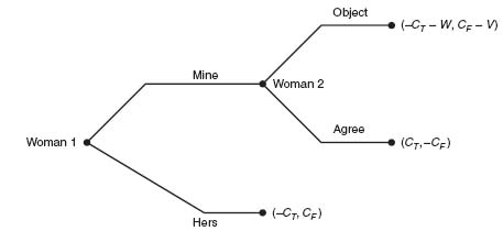
Similarly, assume that woman 2 is the true mother. Then the tree becomes
Woman 2 the true mother
Since CT − V > − CT, woman 2 always Objects if woman 1 calls Mine. Eliminating the Agree branch for woman 2, we now compare (− CF, CT) and (− CF − W, CT − V). Since − CF > − CF − W, we conclude that woman 1 will always call Hers. Backward induction gives us that woman 1 always calls Hers (and if woman 1 calls Mine, then woman 2 Objects). Either way, woman 2, the true mother, ends up with the child.
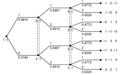
4.9 This is a simple model to see if bluffing is ever optimal. Here is the Ace–Two raise or fold figure.
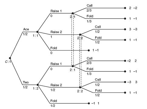
Player I has perfect information but player II only knows if player I has raised $1 or $2, or has folded. This is a zero sum game with value ![]() to player I and −
to player I and − ![]() to player II. The Nash equilibrium is the following.
to player II. The Nash equilibrium is the following.
If player I gets an Ace, she should always Raise $2, while if player I gets a Two, she should Raise $2 50% of the time and Fold 50% of the time. Player II’s Nash equilibrium is if player I Raises $1, player II should Call with probability ![]() and Fold with probability
and Fold with probability ![]() ; if player I Raises $2, then player II should Call 50% of the time and Fold 50% of the time. A variant equilibrium for player II is that if player I Raises $1 then II should Call 100% of the time.
; if player I Raises $2, then player II should Call 50% of the time and Fold 50% of the time. A variant equilibrium for player II is that if player I Raises $1 then II should Call 100% of the time.
4.11 If we use Gambit to solve this game we get the game matrix
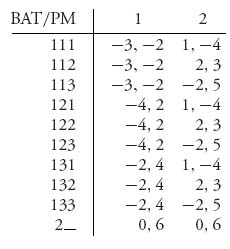
By dominance, the matrix reduces to the simple game
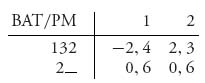
This game has a Nash equilibrium at (0, 6). We will see it is subgame perfect.
The subgame perfect equilibrium is found by backward induction. At node 1:2, BAT will play Out with payoff (− 2, 4) for each player. At 1:3, BAT plays Passive with payoffs (2, 3). At 2:1, PM has the choice of either payoff 4 or payoff 3 and hence plays Tough at 2:1. Now player BAT at 1:1 compares (0, 6) with (− 2, 4) and chooses Out. The subgame perfect equilibrium is thus BAT plays Out, and PM has no choices to make. The Nash equilibrium at (0, 6) is subgame perfect.
4.13 The game tree is given in the figure:
Beer or quiche signalling game—weak probability 0.1
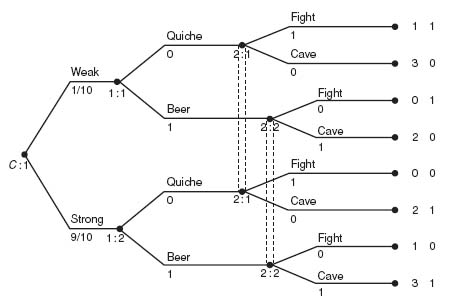
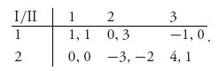
Let’s first consider the equivalent strategic form of this game. The game matrix is
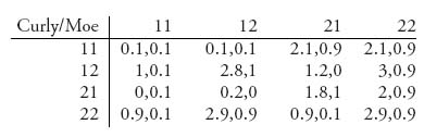
First, note that the first column for player II (Moe) is dominated strictly and hence can be dropped. But that’s it for domination.
There are four Nash equilibria for this game. In the first Nash, Curly always chooses to order quiche, while Moe chooses to cave. This is the dull game giving an expected payoff of 2.1 to Curly and 0.9 to Moe. An alternative Nash is Curly always chooses to order a beer and Moe chooses to cave, giving a payoff of 2.9 to Curly and 0.9 to Moe. It seems that Moe is a wimp.
4.15.a The game tree is in the figure.
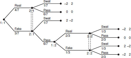
There are three pure strategies for Jack: (1) Real, (2) Fake, then Real and (3) Fake, then Fake. Jill also has three pure strategies: (1) Swat, (2) Pass, then Swat and (3) Pass, then Pass.
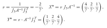
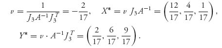
We can use Gambit to solve the problem, but we will use the invertible matrix theorem instead. We get
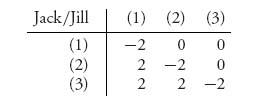
4.15.b Jack and Jill have the same pure strategies but the solution of the game is quite different. The matrix is
For example, (1) versus (1) means Jack will put down the real fly and Jill will try to swat the fly. Jack’s expected payoff is
The game tree from the first part is easily modified noting that the probability of hitting or missing the fly only applies to the real fly. Here is the figure with Gambit’s solution below the branches.
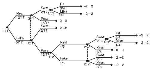
The solution of the game is
4.17 Using Maple, we have
 > restart:A: = Matrix([[1, 1, 1, 1], [0, 3, 3, 3], [0, 2, 5, 5], [0, 2, 4, 7]]);
 > B: = Matrix([[0, 0, 0, 0], [3, 2, 2, 2], [3, 5, 4, 4], [3, 5, 7, 6]]);
 > P: = Matrix(4, 4, symbol = p);
 > Z: = add(add((A[i, j] + B[i, j])*p[i, j], i = 1..4), j = 1..4):
 > with(simplex):
 > cnsts: = {add(add(p[i, j], i = 1..4), j = 1..4) = 1}:
 > for i from 1 to 4 do
               for k from 1 to 4 do
                cnsts: = cnsts union {add(p[i, j]*A[i, j], j = 1..4) > =
                          add(p[i, j]*A[k, j], j = 1..4)}:
                end do:
end do:
 > for j from 1 to 4 do
                 for k from 1 to 4 do
               cnsts: = cnsts union {add(p[i, j]*B[i, j], i = 1..4) > =
                        add(p[i, j]*B[i, k], i = 1..4)}:
               end do:
end do:
 > maximize(Z, cnsts, NONNEGATIVE);
 > with(Optimization):
 > LPSolve(Z, cnsts, assume = nonnegative, maximize);
The result is p1, 1 = 1 and pi, j = 0 otherwise. The correlated equilibrium also gives the action that each player Stops.
4.19 This problem can be tricky because it quickly becomes unmanageable if you try to solve it by considering all possibilities. The key is to recognize that after the first round, if all three stooges survive it is as though the game starts over. If only two stooges survive, it is like a duel between the survivors with only one shot for each player and using the order of play Larry, then Moe, then Curly (depending on who is alive).
According to the instructions in the problem we take the payoffs for each player to be 2, if they are sole survivor, ![]() if there are two survivors, 0 if all three stooges survive and −1 for the particular stooge who is killed. The payoffs at the end of the first round are −1 to any killed stooge in round 1, and the expected payoffs if there are two survivors, determined by analyzing the two person duels first. This is very similar to using backward induction and subgame perfect equilibria.
if there are two survivors, 0 if all three stooges survive and −1 for the particular stooge who is killed. The payoffs at the end of the first round are −1 to any killed stooge in round 1, and the expected payoffs if there are two survivors, determined by analyzing the two person duels first. This is very similar to using backward induction and subgame perfect equilibria.
Begin by analyzing the two person duels Larry vs. Moe, Moe vs. Curly, and Curly vs. Larry. We assume that round one is over and only the two participants in the duel survive. We need that information in order to determine the payoffs in the two person duels. Thus, if Larry kills Curly, Larry is sole survivor and he gets 2, while Curly gets −1. If Larry misses, he’s killed by Curly and Curly is sole survivor.
1. Curly versus Larry:
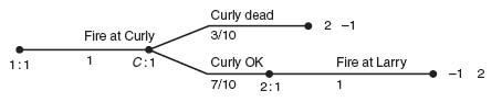
In this simple game, we easily calculate the expected payoff to Larry is − ![]() and to Curly is
and to Curly is ![]() .
.
2. Moe versus Curly:
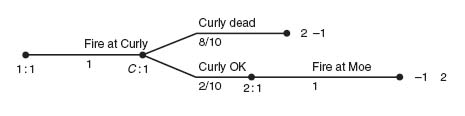
The expected payoff to Moe is ![]() , and to Curly is −
, and to Curly is − ![]() .
.
3. Larry versus Moe:
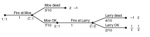
In this case, if Larry shoots Moe, Larry gets 2 and Moe gets −1, but if Larry misses Moe, then Moe gets his second shot. If Moe misses Larry, then there are two survivors of the truel, and each gets ![]() . The expected payoff to Moe is
. The expected payoff to Moe is ![]() , and to Curly is −
, and to Curly is − ![]() .
.
Next consider the tree below for the first round incorporating the expected payoffs for the second round.
The expected payoff to Larry is 0.68, Moe is 0.512, and Curly is 0.22. The Nash equilibrium says that Larry should deliberately miss with his first shot. Then Moe should fire at Curly; if Curly lives, then Curly should fire at Moe–and Moe dies. In the second round, Larry has no choice but to fire at Curly, and if Curly lives, then Curly will kill Larry.
Does it make sense that Larry will deliberately miss in the first round? Think about it. If Larry manages to kill Moe in the first round, then surely Curly kills Larry when he gets his turn. If Larry manages to kill Curly, then with 80% probability, Moe kills Larry. His best chance of survival is to give Moe and Curly a chance to shoot at each other. Since Larry should deliberately miss, when Moe gets his shot he should try to kill Curly because when it’s Curly’s turn, Moe is a dead man.
To find the probability of survival for each player assuming the Nash equilibrium is being played we calculate:
1. For Larry:
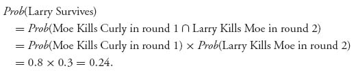
2. For Moe:
3. For Curly:
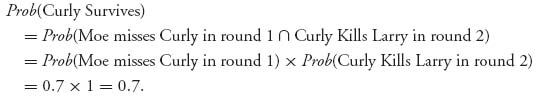
First round tree using second round payoffs.
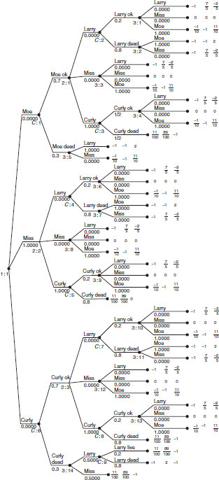
4.21 Here is the figure:
Two-stage centipede with altruism
The expected payoffs to each player are ![]() for I and
for I and ![]() for II. The Nash equilibrium is the following.
for II. The Nash equilibrium is the following.
If both players are rational, I should Pass, then II should Pass with probability ![]() , then I should Pass with probability
, then I should Pass with probability ![]() , then player II should Pass with probability 0.
, then player II should Pass with probability 0.
If I is rational and II is an altruist, then I should Pass with probability 1, then II Passes, then I Passes with probability ![]() , then II Passes.
, then II Passes.
If I is an altruist and II is rational, then I Passes, II Passes with probability ![]() , I Passes, and II Passes with probability 0.
, I Passes, and II Passes with probability 0.
If they are both altruists, they each Pass at each step and go directly to the end payoff of 12.80 for I and 3.20 for II.
Solutions for Chapter 5
5.1.a Since ![]() maximizes both u1 and u2, we have
maximizes both u1 and u2, we have
![]()
Thus,
![]()
for every ![]() Thus,
Thus, ![]() automatically satisfies the definition of a Nash equilibrium. A maximum of both payoffs is a much stronger requirement than a Nash point.
automatically satisfies the definition of a Nash equilibrium. A maximum of both payoffs is a much stronger requirement than a Nash point.
5.1.b Consider ![]() and
and ![]() and −1 ≤ q1 ≤ 1, −1 ≤ q2 ≤ 1.
and −1 ≤ q1 ≤ 1, −1 ≤ q2 ≤ 1.
The function ![]()
There is a unique Nash equilibrium at ![]() since
since
![]()
gives ![]() and these points provide a maximum of each function with the other variable fixed because the second partial derivatives are −2 < 0. On the other hand,
and these points provide a maximum of each function with the other variable fixed because the second partial derivatives are −2 < 0. On the other hand,
![]()
Thus, ![]() maximizes neither of the payoff functions. Furthermore, there does not exist a point that maximizes both u1, u2 at the same point (q1, q2).
maximizes neither of the payoff functions. Furthermore, there does not exist a point that maximizes both u1, u2 at the same point (q1, q2).
5.3.a By taking derivatives, we get the best response functions
The graphs of the rational reaction sets are as follows:
The function ![]()
5.3.b The rational reaction sets intersect at the unique point (x*, y*) = (2, 2), which is the unique pure Nash equilibrium.
5.5 We claim that if N ≤ 4, then (0, 0, …, 0) is a Nash equilibrium. In fact, u1(0, 0, 0, 0) = 0 but ![]() Similarly for the remaining cases.
Similarly for the remaining cases.
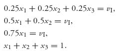
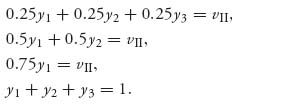
5.7 According to the solution of the median voter problem in Example 5.3 we need to find the median of X. To do that we solve for γ in the equation:
![]()
This equation becomes −0.41 γ3 + γ2 + 0.41 γ − 0.5 = 0 which implies γ = 0.585. The Nash equilibrium position for each candidate is (γ*, γ*) = (0.585, 0.585). With that position, each candidate will get 50% of the vote.
5.9 The best responses are easily found by solving ![]() and
and ![]() The result is
The result is
![]()
and solving for x and y results in x = 4, y = 4 as the Nash equilibrium. The payoffs are u1(4, 4) = u2(4, 4) = 16.
5.11 Calculate the derivatives and set to zero: ![]() is the best response. Similarly,
is the best response. Similarly, ![]() The Nash equilibrium is then
The Nash equilibrium is then ![]() assuming that 2w1 > w2, 2w2 > w1. If w1 = w2 = w, then
assuming that 2w1 > w2, 2w2 > w1. If w1 = w2 = w, then ![]() and each citizen should donate one-third of their wealth.
and each citizen should donate one-third of their wealth.
5.13 The payoffs are
First, calculate maxt1≥0 u1(t1, t2) and maxt2≥0 u2(t1, t2). For example,
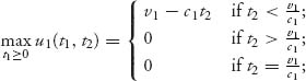
and the maximum is achieved at the set valued function
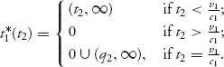
This is the best response of country 1 to t2. Next, calculate the best response to t1 for country 2, ![]()
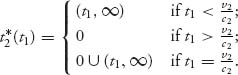
If you now graph these sets on the same set of axes, the Nash equilibria are points of intersection of the sets. The result is
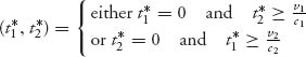
For example, this says that either (1) country 1 should concede immediately and country 2 should wait until first time ![]() or (2) country 2 should concede immediately and country 1 should wait until first time
or (2) country 2 should concede immediately and country 1 should wait until first time ![]()
5.15.a If three players take A → B → C, their travel time is 51. No player has an incentive to switch. If 4 players take this path, their travel time is 57 while the two players on A → D → C travel only 45, clearly giving an incentive for a player on A → B → C to switch.
5.15.b If 3 cars take the path A → B → D → C their travel time is 32 while if the other 3 cars stick with A → D → C or A → B → C, the travel time for them is still 51, so they have an incentive to switch. If they all switch to A → B → D → C, their travel time is 62. If 5 cars take A → B → D → C their travel time is 52 while the one car that takes A → D → C or A → B → C has travel time 33 + 31 = 64. Note that no player would want to take A → D → B → C because the travel time for even one car is 66. Continuing this way, we see that the only path that gives no player an incentive to switch is A → B → D → C. That is the Nash equilibrium and it results in a travel time that is greater than before the new road was added.
5.17 We have the derivatives
![]()
and
![]()
and hence, concavity in the appropriate variable for each payoff function. Solving the first derivatives set to zero gives
![]()
Then
![]()
5.19 For each player i, let xi be the choice of integer from 1 to 100. The payoff function can be written as
We need to show that
![]()
Recall that 1−i denotes that all the players except player i are playing 1. Note that since ![]() when all players choose 1,
when all players choose 1, ![]() and
and ![]() What is a better xi for player i to switch to? In order to be better it must satisfy
What is a better xi for player i to switch to? In order to be better it must satisfy
![]()
Note that ![]() Hence, we must have
Hence, we must have
![]()
That is impossible. Hence, (1, 1, …, 1) is a Nash equilibrium.
5.21 The price subsidy kicks in if ![]() which implies that the total quantity shipped, Q = q1 + q2 + q3 ≤ 1, 950, 000. The price per bushel is given by
which implies that the total quantity shipped, Q = q1 + q2 + q3 ≤ 1, 950, 000. The price per bushel is given by
![]()
Each farmer has the payoff function
![]()
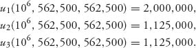
Assume that Q < 1, 950, 000. Take a partial derivative and set to zero to get qi = 562, 500 bushels each. Then Q = 1, 687, 500 < 1, 950, 000. So an interior pure Nash equilibrium consists of each farmer sending 562, 500 bushels each to market and using 437, 500 bushels for feed. The price per bushel will be ![]() which is greater than the government-guaranteed price.
which is greater than the government-guaranteed price.
If each producer ships 562, 500 bushels, the profit for each producer is
![]()
Now suppose producer 1 ships his entire crop of q1 = 106 bushels. Assuming the other producers are not aware that producer 1 is shipping 106 bushels. If the other producers still ship 562, 500 bushels the total shipped will be 2, 125, 000 > 1, 950, 000 and the price per bushel would be subsidized at 2. The revenue to each producer is then
This means all the producers make less money but 2 and 3 make significantly less.
It’s very unlikely that 2 and 3 would be happy with this solution. We need to find 2 and 3’s best responses to 1’s shipment of 106. Assume first that 106 + q2 + q3 ≤ 1, 950, 000. We calculate
![]()
The problem for q3 is similar. Taking a derivative, setting to zero, and solving for q2, q3 results in q2 = q3 = (1.25 × 10⁶)/3 = 416, 667. That is the best response of producers 2 and 3 to producer 1 shipping his entire crop assuming Q ≤ 1, 950, 000. The price per bushel at total output 1, 833, 334 bushels will be $2.78 and the profit for each producer will be u1 = 2, 780, 000, u2 = u3 = 1, 158, 334.
Now assume that Q ≥ 1, 950, 000. In this case, p = 2 and the profit for each producer is u1 = 2, 000, 000, u2 = 2 × q2, u3 = 2 × q3. The maximum for producers 2 and 3 is achieved with q2 = q3 = 106 and all 3 producers ship their entire crop to market. This is clearly the best response of producers 2 and 3 to q1 = 106.
5.23.a If we take the first derivatives, we get
![]()
The second partials give us
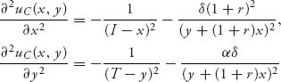
both of which are < 0. That means that we can find the Nash equilibrium where the first partials are zero. Solving, we get the general solution
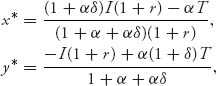
and that is the Nash equilibrium as long as 0 ≤ x* < I, 0 ≤ y* < T.
5.23.b For the data given in the problem x* = 338.66, y* = 357.85.
5.25.a
5.25.b If y < 1, then investor I would like to choose an x ![]() (y, 1) (in particular we want to choose x = y but y
(y, 1) (in particular we want to choose x = y but y ![]() (y, 1)), and therefore, no best response exists. If x < 1, then investor II would like to choose a y
(y, 1)), and therefore, no best response exists. If x < 1, then investor II would like to choose a y ![]() (x, 1) and II has no best response either. The last case is x = y = 1. In this case, both investors have best responses x = 0 or y = 0.
(x, 1) and II has no best response either. The last case is x = y = 1. In this case, both investors have best responses x = 0 or y = 0.
5.25.c First, observe that u1(x, y) = u2(y, x) that means that if X is a Nash equilibrium for player I, then it is also a Nash equilibrium for player II. From the definition of ![]() so that taking derivatives,
so that taking derivatives,
![]()
Now since ![]() we conclude that g(x) = 1, 0 ≤ x ≤ 1. This is the density for a uniformly distributed random variable on [0, 1]. Thus, the Nash equilibrium is that each investor chooses an investment level at random.
we conclude that g(x) = 1, 0 ≤ x ≤ 1. This is the density for a uniformly distributed random variable on [0, 1]. Thus, the Nash equilibrium is that each investor chooses an investment level at random.
Finally, we will see that vI = vII = 0. But that is immediate from
![]()
5.27.a If they have the same unit costs, the two firms together should act as a monopolist. This means the optimal production quantities for each firm should be
![]()
The payoffs to each firm is then ![]() which is greater than the profit under competition. Furthermore, the cartel price will be the same as the monopoly price since the total quantity produced is the same.
which is greater than the profit under competition. Furthermore, the cartel price will be the same as the monopoly price since the total quantity produced is the same.
5.27.b The best response of firm 1 to the quantity ![]() is given by
is given by
![]()
Thus firm 1 should produce more than firm 2 as a best response. Similarly, firm 2 has an incentive to produce more than firm 1. The cartel collapses.
5.29 The profit function for firm i is ![]() If we take derivatives and set to zero, we get
If we take derivatives and set to zero, we get
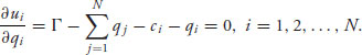
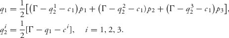
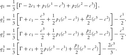
Since ![]() any critical point will provide a maximum. Set αi = Γ − ci. We have to solve the system of equations
any critical point will provide a maximum. Set αi = Γ − ci. We have to solve the system of equations ![]() In matrix form, we get the system
In matrix form, we get the system
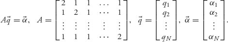
It is easy to check that
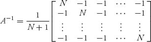
and then
![]()
After a little algebra, we see that the optimal quantity that each firm should produce is
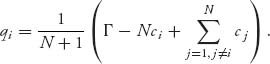
If ci = c, i = 1, 2, …, N, then ![]() The profits then also approach zero.
The profits then also approach zero.
5.31.a No firm would produce more than 10 because the cost of producing and selling one gadget would essentially be the same as the return on that gadget.
5.31.b The profit function for the monopolist is
![]()
Taking a derivative and setting to zero gives
![]()
and it is easy to check that ![]() provides the maximum. Also
provides the maximum. Also ![]()
5.31.c Now we have
![]()
We can take advantage of the fact that there is symmetry between the two firms since they have the same price function and costs. That means, for firm 1,
![]()
The maximum is achieved at ![]() s Thus, the Nash equilibrium is
s Thus, the Nash equilibrium is ![]() and
and ![]()
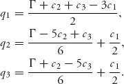
5.33.a We have to solve the system
Observe that q1 is the expected value of the best response production quantities when the costs for firm 2 are ci, i = 1, 2, 3 with probability pi, i = 1, 2, 3. The system of best response equations has following solution:
5.33.b The optimal production quantities with the information given are ![]() for firm 1, and
for firm 1, and ![]() and
and ![]()
5.35 First, we have to find the best response functions for firms 2 and 3. We have from the profit functions and setting derivatives to zero,
![]()
Solving these two equation results in
![]()
Next, firm 1 will choose q1 to maximize
![]()
Taking a derivative and setting to zero, we get ![]() Finally, plugging this q1 into the best response functions q2, q3, we get the optimal Stackelberg production quantities:
Finally, plugging this q1 into the best response functions q2, q3, we get the optimal Stackelberg production quantities:
The profits for each firm are as follows:
5.37 If c1 = c2 = c, we have the profit function for firm 2:
We will show that u2(c, c) ≥ u2(c, p2), for any p2 ≠ c. Now, u2(c, c) = 0 and
In every case u2(c, c) = 0 ≥ u2(c, p2). Similarly u1(c, c) ≥ u1(p1, c) for every p1 ≠ c. This says (c, c) is a Nash equilibrium and both firms make zero profit.
5.39 The profit functions for each firm are as follows:
and
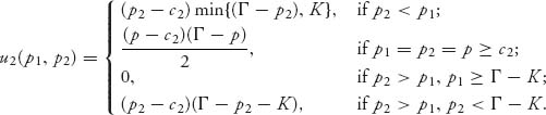
To explain the profit function for firm 1, if p1 < p2, firm 1 will be able to sell the quantity of gadgets q = min{Γ − p1, K}, the smaller of the demand quantity at price p1 and the capacity of production for firm 1.
If p1 = p2, so that both firms are charging the same price, they split the market and since ![]() there is enough capacity to fill the demand.
there is enough capacity to fill the demand.
If p1 > p2 in the standard Bertrand model, firm 1 loses all the business since they charge a higher price for gadgets. In the limited capacity model, firm 1 loses all the business only if, in addition, p2 ≥ Γ − K; that is, if K ≥ Γ − p2, which is the amount that firm 2 will be able to sell at price p2, and this quantity is less than the production capacity.
Finally, if p1 > p2, and K < Γ − p2, firm 1 will be able to sell the amount of gadgets that exceed the capacity of firm 2. That is, if K < Γ − p2, then the quantity demanded from firm 2 at price p2 is greater than the production capacity of firm 2 so the residual amount of gadgets can be sold to consumers by firm 1 at price p1. But note that in this case, the number of gadgets that are demanded at price p1 is Γ − p1, so firm 1 can sell at most Γ − p1− K < Γ − p2 − K.
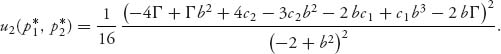
What about Nash equilibria? Even in the case c1 = c2 = 0 there is no pure Nash equilibrium even at ![]() This is known as the Edgeworth paradox.
This is known as the Edgeworth paradox.
5.41 Start with profit functions
![]()
Solve ![]() to get the best response function:
to get the best response function:
![]()
Next, solve ![]() to get
to get
![]()
and then, the optimal price for firm 2 is
![]()
The profit functions become
![]()
and
Note that with the Stackelberg formulation and the formulation in the preceding problem the Nash equilibrium has positive prices and profits.
The Maple commands to do these calculations are as follows:
> u1:=(p1, p2)->(G-p1+b*p2)*(p1-c1);
> u2:=(p1, p2)->(G-p2+b*p1)*(p2-c2);
> eq1:=diff(u2(p1, p2), p2)=0;
> solve(eq1, p2);
> assign(p2, %);
> f:=p1->u1(p1, p2);
> eq2:=diff(f(p1), p1)=0;
> solve(eq2, p1);
> simplify(%);
> assign(p1, %);
> p2;simplify(%);
> factor(%);
> assign(a2, %);
> u1(p1, a2);
> simplify(%);
> u2(p1, a2);
> simplify(%);
For the data of the problem, we have
![]()
5.43 The payoff functions are as follows:
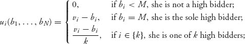
and recall that v1 ≥ v2 ··· ≥ vN. We have to show that ui(v1, …, vN) gives a larger payoff to player i if player i makes any other bid bi ≠ vi. We assume that v1 = v2 so the two highest valuations are the same. Now for any player i if she bids less than v1 = v2 she does not win the object and her payoff is zero. If she bids bi > v1 she wins the object with payoff vi − bi < v1 − bi < 0. If she bids bi = v1, her payoff is ![]() In all cases, she is worse off if she deviates from the bid bi = vi as long as the other players stick with their valuation bids.
In all cases, she is worse off if she deviates from the bid bi = vi as long as the other players stick with their valuation bids.
5.45 In the first case, it will not matter if she uses a first or second price auction. Either way she will sell it for $100, 000. In the second case, the winning bid for player 1 is between 95, 000 < b1 < 100, 000 whether it is a first or second price auction. However, in the second price auction, the house will sell for $95, 000. Thus, a first price auction is better for the seller.
5.47 The expected payoff of a bidder with valuation v who makes a bid of b is given by
![]()
Differentiate, set to zero, and solve to get ![]()
Since all bidders will actually pay their own bids and each bid is ![]() the expected payment from each bidder is
the expected payment from each bidder is
![]()
Since there are N bidders, the total expected payment to the seller will be ![]()
Solutions for Chapter 6
6.1.a The normalized function is ![]()
6.1.b The core using v′ is
The unnormalized allocations satisfy

Since 1 − nα > 0, xi − α ≥ 0 and ![]() In terms of the unnormalized allocations,
In terms of the unnormalized allocations, ![]()
6.3 Let ![]() Calculate for
Calculate for ![]()
![]()
Since b < nc and n > |S| both terms in the max are negative so ![]() If S = N,
If S = N,
![]()
since b < nc. By definition, we conclude ![]()
6.5 The characteristic function is
![]()
The normalized characteristic function is
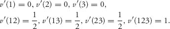
The normalized least core is ![]() The unnormalized least core is
The unnormalized least core is ![]()
The normalized least core comes from the inequalities
![]()
which decides ![]() is the first ε. Then
is the first ε. Then ![]() Then
Then ![]() implies
implies ![]() and hence
and hence ![]()
6.7 In normalized form since v(i) = 0, simply divide each allocation value by v(1234) = 13: ![]()
6.9 ![]() v(2) = 2, v(3) = 1, v(12) = 5, v(13) = 4, v(23) = 3, v(123) = 16.
v(2) = 2, v(3) = 1, v(12) = 5, v(13) = 4, v(23) = 3, v(123) = 16.
6.11 Writing out the inequalities for C(ε) we have the inequalities
![]()
and x1 + x2 + x3 = 4. These imply that 3 − ε ≤ x1 + x2 ≤ 5 + ε and then −2 ≤ 2ε. Consequently, we derive that ε1 = −1 and the least core is ![]()
6.13 Suppose ![]() so that
so that ![]() Take the single player coalition S = {i} so v(i) + v(N − i) = v(N). Since the game is essential,
Take the single player coalition S = {i} so v(i) + v(N − i) = v(N). Since the game is essential, ![]() Since
Since ![]() is in the core, we have
is in the core, we have
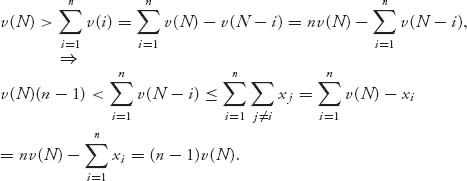
That’s a contradiction, and hence C(0) = ![]() .
.
6.15 Suppose i = 1. Then
![]()
and so x1 ≤ 0. But since −x1 = v(1) − x1 ≤ 0, we have x1 = 0.
6.17 Let ![]() Since v(N − 1) ≤ x2 + ··· + xn = v(N) − x1, we have x1 ≤ v(N) − v(N − 1). In general, xi ≤ v(N) − v(N − i), 1 ≤ i ≤ n. Now add these up to get v(N) = ∑i xi ≤ ∑i δi < v(N), which says C(0) =
Since v(N − 1) ≤ x2 + ··· + xn = v(N) − x1, we have x1 ≤ v(N) − v(N − 1). In general, xi ≤ v(N) − v(N − i), 1 ≤ i ≤ n. Now add these up to get v(N) = ∑i xi ≤ ∑i δi < v(N), which says C(0) = ![]() .
.
6.19 If we remove, say player 1 from N, then N − 1 has 2n−1 coalitions (including the empty coalition), none of which contain player 1. But N has 2n coalitions and so the number of coalitions that do not contain player 1 is 2n − 2n−1 = 2n−1 and consequently there are 2n−1 coalitions that do contain player 1.
6.21.a The characteristic function for this game is
![]()
For example, for S = 1, players 2 and 3 get their capacity first which is 135; the 15 left over go to player 1.
6.21.b If we find the least core and show that ε1 < 0, then it must be true that C(ε1) ⊂ C(0) ≠ ![]() . The least core inequalities we must solve are as follows:
. The least core inequalities we must solve are as follows:
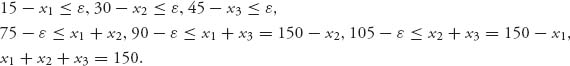
Hence, x2 ≤ 60 + ε, x1 ≤ 45 + ε ⇒ 75 − ε ≤ x1 + x2 ≤ 105 + 2ε that gives ε1 = −10. Then x1 + x2 = 85, x3 = 65, and since x1 ≤ 35, x2 ≤ 50, it must be true that x1 = 35, x2 = 50. The least core is C(−10) = {(35, 50, 65)} the exact same allocation as before but with a nonempty core. Every player is ok with this allocation.
6.23.a The payoff for player i is the number of bags of garbage dumped in his yard times −1. The payoff for a coalition is the number of bags of garbage dumped on all the yards of members of S times −1. If there are n players, there are n − |S| bags of garbage that will be dumped on the yards of the coalition S.
6.23.b Suppose n > 2 and C(0) ≠ ![]() . Since v(S) = |S| − n ≤ ∑j
. Since v(S) = |S| − n ≤ ∑j![]() S xj we have for any k = 1, 2, …, n, −1 = v(N − k) ≤ ∑j
S xj we have for any k = 1, 2, …, n, −1 = v(N − k) ≤ ∑j![]() N−k xj. This says
N−k xj. This says
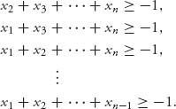
Add these up and use the fact that ![]() to get the requirement
to get the requirement
![]()
With this contradiction, we see that n > 2 ⇒ C(0) = ![]() .
.
Another way to see this is to use a result from an earlier Problem 6.17 that gives us a criterion to use to determine when the core is empty. The criterion says
![]()
In the garbage game, we have
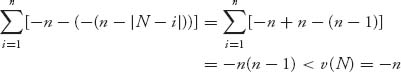
implies that n − 1 > 1 or n > 2. We conclude that when n > 2, from Problem 6.17, the core of the garbage game is empty.
6.23.c A coalition that works is S = {12}.
6.25.a v(![]() ) = 0, v(1) = −100, v(2) = −150, v(3) = −400, v(12) = −150, v(13) = −400, v(23) = −400, v(123) = −400.
) = 0, v(1) = −100, v(2) = −150, v(3) = −400, v(12) = −150, v(13) = −400, v(23) = −400, v(123) = −400.
6.25.b The least ε −core is given by
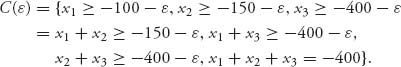
Next,
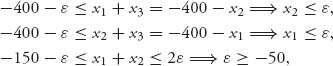
and that gives us the first ε1 = −50. This implies
![]()
6.27 We have
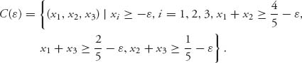
Checking all possible combinations of inequalities results in the first ε from the inequalities
![]()
and ![]() Then, the first least core is
Then, the first least core is
![]()
Next, we calculate the excesses for ![]()
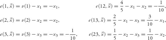
Thus, we may eliminate coalitions 3 and 12 since their excesses cannot be reduced further. The next least core is
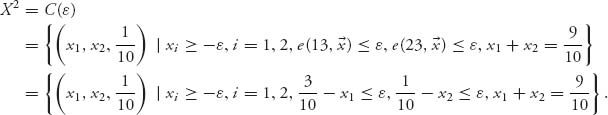
We get
![]()
The first ε making ![]() Then we calculate the next least core is
Then we calculate the next least core is ![]() This contains only one point and is the nucleolus.
This contains only one point and is the nucleolus.
6.29 The characteristic function can be taken to be the interest earned on the investment:
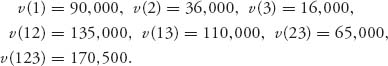
To get the least core, we have
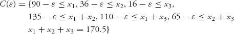
Using the inequalities 90 − ε ≤ x1 ≤ 105.5 − ε, we get the first ![]() Then x1 = 97.75 and x2 + x3 = 72.75.
Then x1 = 97.75 and x2 + x3 = 72.75.
We need the next least core. We calculate the excesses for ![]() to get
to get
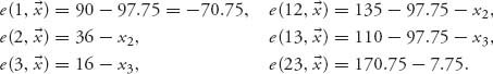
The next least core will work with coalitions {2, 3, 12, 13} since only those coalitions have excesses which may be lowered. We have
![]()
The two inequalities 16 − x3 ≤ ε, 37.25 − x2 ≤ ε lead to 53.25 − 2ε ≤ x2 + x3 = 72.75 and ε2 = −9.75 as the first ε making X2 ≠ ![]() . Then 37.25 + 9.75 = 47 ≤ x2, and 16 + 9.75 = 25.75 ≤ x3 imply that x2 = 47, x3 = 25.75.
. Then 37.25 + 9.75 = 47 ≤ x2, and 16 + 9.75 = 25.75 ≤ x3 imply that x2 = 47, x3 = 25.75.
The nucleolus is ![]()
It is interesting to compare this with the common assumption that the fair allocation should be that each player will get the amount of 170, 500 proportional to the amount they invest. That would lead to the allocation ![]() 170, 500 = 108063.38, and
170, 500 = 108063.38, and ![]() 170, 500 = 43225.35, and
170, 500 = 43225.35, and ![]() 170, 500 = 19211.27. But, this does not take into account that player 3 is a very important investor. It is her money that pushes the grand coalition into the 5.5% rate of return. Without player 3 the most they could get is 5%. Consequently, player 3 has to be compensated for this power. The proportional allocation doesn’t do that.
170, 500 = 19211.27. But, this does not take into account that player 3 is a very important investor. It is her money that pushes the grand coalition into the 5.5% rate of return. Without player 3 the most they could get is 5%. Consequently, player 3 has to be compensated for this power. The proportional allocation doesn’t do that.
6.31.a Let’s draw an appointment schedule:
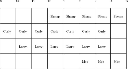
The characteristic function is the number of hours saved by a coalition. Single coalitions save nothing v(i) = 0, i = 1, 2, 3, 4, and
![]()
For instance v(124) = 7 since Shemp and Curly overlap 4 hours and Shemp and Moe overlap 3 hours.
6.31.b We will use either Maple or Mathematica to solve this problem. We show that the ![]() with units in hours.
with units in hours.
The first least core is determined from ![]()
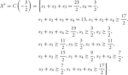
A decided allocation is ![]() Next, to get X2 first calculate the excesses
Next, to get X2 first calculate the excesses ![]() for
for ![]() and we see that we may eliminate coalitions S = 4, S = 123.
and we see that we may eliminate coalitions S = 4, S = 123.
We then obtain ![]() and
and ![]() Again we calculate the excesses
Again we calculate the excesses ![]() and we determine we may eliminate coalitions S = 1, S = 14, S = 1234.
and we determine we may eliminate coalitions S = 1, S = 14, S = 1234.
Finally, we calculate ![]() using only the coalitions S = 2, 3, 124, 134, and we get
using only the coalitions S = 2, 3, 124, 134, and we get ![]() That is the nucleolus.
That is the nucleolus.
6.31.c The schedule is set up as follows:
6.33 The characteristic function for the savings game is v(![]() ) = 0, v(i) = 0, v(1234) = 22 − 8.5, and
) = 0, v(i) = 0, v(1234) = 22 − 8.5, and
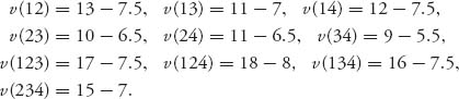
The least core is
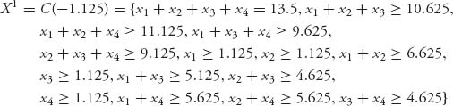
This reduces to ![]() so this is the nucleolus.
so this is the nucleolus.
In the original terms of costs, we have
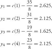
6.35 We have T ![]() 2N Πi if and only if T ∪ i
2N Πi if and only if T ∪ i ![]() Πi. Also, |T ∪ i| = |T| + 1. Hence,
Πi. Also, |T ∪ i| = |T| + 1. Hence,
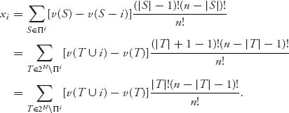
6.37.a A reasonable characteristic function is
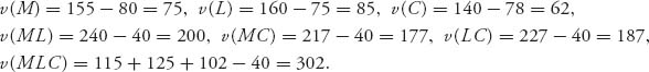
6.37.b The Mathematica statements to find the least core are very simple:
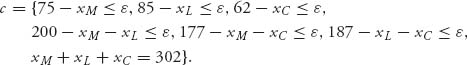
Then
![]()
Of course, this can also be done tediously by hand. The result is
![]()
and that’s one fair way to divide the total of 302.
6.37.c We calculate the Shapley value from the table:
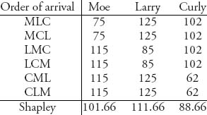
The Shapley allocation is the same as the nucleolus. Looks like waxing is lucrative.
6.39 Take the characteristic function representing the hours saved by a coalition,
![]()
Then the nucleolus is C(−1) = {(1, 1, 2)}. Thus, Moe and Curly both save 1 hour while Larry saves 2. Since Curly arrives first, he can now work 9-12. Then Larry works 12-3, and Moe works 3-5.
The Shapley allocation is the same as the least core. For example,
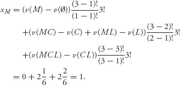
Here is the table giving the Shapley allocation:
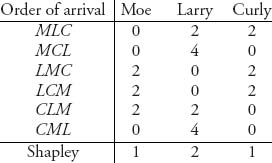
6.41.a The characteristic function is v(i) = 0, v(12) = 100, v(13) = 130, v(23) = 0, v(123) = 130. We calculate the core,
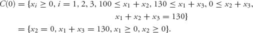
The Shapley value is ![]() and this point is not in C(0) since
and this point is not in C(0) since ![]() and
and
![]()
The nucleolus of this game is {(115, 0, 15)} which is quite different from the Shapley value. Under the nucleolus, of the 130 available if the players cooperate, the seller gets 115 for her object, and player 3 gets to keep 15 of her 130. She pays the seller 115. Under Shapley, the seller gets 81.67, player 3 pays a total of 130-31.67 = 98.33 of which 81.67 goes to the seller to buy the object and 16.67 goes to player 2 to go away. Do you think this is what would actually happen?
6.41.b To be individually rational, we need v(i) ≤ xi, i = 1, 2, 3 that is clearly satisfied for the Shapley value. The group rational condition requires ![]() In our case,
In our case,
![]()
6.43 Shapley ![]()
6.45 The Shapley value for the game is (−1, −1, −1, −1). To see why, since the game is symmetric clearly the formula for the Shapley value will give x1 = x2 = x3 = x4. Since x1 + x2 + x3 + x4 = v(N) = −4, we must have x1 = x2 = x3 = x4 = −1.
6.47 Shapley value = {(3.91667, 3.66667, 2.75, 3.16667)}.
6.49.a The characteristic function is
![]()
6.49.b The core is C(0) = {(2, 0, 0, 0)}. To see this,
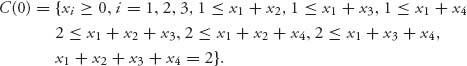
Adding the three-player coalitions, we see that
![]()
Then x1 + x2 + x3 + x4 = 2 ⇒ x1 = 2, x2 = x3 = x4 = 0. Thus, C(0) = {(2, 0, 0, 0)}.
Since the core contains only one point, it is the nucleolus. Player 1 is allocated everything while players 2, 3, and 4 get nothing. Doesn’t seem fair.
6.49.c Players 2, 3, and 4 are symmetric so the Shapley allocation is of the form (x, y, y, y), where x + 3y = 2. By the formula for the Shapley value,
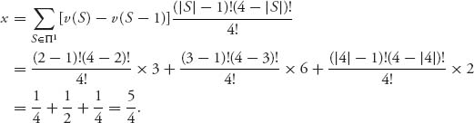
Then ![]() The Shapley value is then
The Shapley value is then ![]()
6.49.d The characteristic function is v(1) = v(2) = 10, v(12) = 30. The core is
![]()
which has more than one point. That means we have to calculate the least core:
![]()
Thus, ε ≥ −5 ⇒ ε1 = −5 ⇒ x1 = x2 = 15 and C(−5) = {(15, 15)}, an even split.
The Shapley allocation is
![]()
which is the same as the nucleolus.
6.51 If n = 5, b = 3, c = 2, we have
![]()
A direct calculation shows that
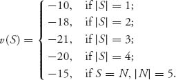
Plugging into Shapley’s formula gives ![]()
6.53.a Since
![]()
we compute
![]()
This characteristic function is superadditive, and they all have an incentive to join the carpool.
6.53.b The inequalities we need to solve are as follows:
![]()
Eliminating x3 we get x2 ≤ 12 + ε, x1 ≤ 15 + ε ⇒ 13 − ε ≤ x1 + x2 ≤ 27 + 2ε. This leads to ![]() and then
and then ![]()
Then ![]() Since 31 + 22 = 53, we conclude
Since 31 + 22 = 53, we conclude ![]() Thus,
Thus,
![]()
6.53.c It seems reasonable that Larry and Curly should pay Moe the difference in the amount it costs them to drive on their own and the amount of the savings attributable to that player. We get Larry should pay Moe ![]() and Curly should pay Moe
and Curly should pay Moe ![]()
6.53.d The table for calculation of the Shapley value is given below.
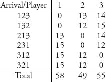
The Shapley allocation is, therefore, ![]() We get Larry should pay Moe
We get Larry should pay Moe ![]() and Curly should pay Moe
and Curly should pay Moe ![]()
6.53.e Let Shemp be player 4. The costs are as follows:
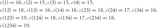
The corresponding cost savings are as follows:
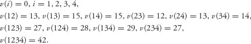
By going through similar calculations, we get
![]()
The Shapley value is
![]()
Larry, Curly, and Shemp should pay Moe the difference in the amount it costs them to drive on their own and the amount of the savings attributable to that player.
6.55 One simple way to calculate the Banzhaf–Coleman index is to list for each coalition, the players who are critical for that coalition (critical means win with the player, lose without her). The table contains the results
| Coalition | Votes | Critical players |
| 12 | 6 | 1, 2 |
| 13 | 5 | 1, 3 |
| 14 | 5 | 1, 4 |
| 123 | 7 | 1 |
| 124 | 7 | 1 |
| 134 | 6 | 1 |
| 1234 | 8 | 1 |
Next, count up the number of times each player is critical for a coalition. For player 1 it is 7 times; player 2, 3, and 4, exactly 1 time each. The total number of winning coalitions for each critical player is 10. Hence,
![]()
Player 1’s power index is 7 times that of the other players even though she has only twice as many votes (as player 2).
6.57.a The matrices are ![]() Calculate easily that value(A) = value(BT) = 0, and hence, the security point is (0, 0). The Nash bargaining problem is then
Calculate easily that value(A) = value(BT) = 0, and hence, the security point is (0, 0). The Nash bargaining problem is then
![]()
By calculus, the solution is ![]() The bargained solution is that each contestant should Split. That seems fair and natural.
The bargained solution is that each contestant should Split. That seems fair and natural.
6.57.b First, we calculate the threat security point. Since the Pareto-optimal boundary is u + v = 1, we have v = −u + 1 and so mp = −1, b = 1. Then we calculate ![]() and value(A − B) = 0, with a saddle point Xt = (0, 1), Yt = (0, 1). The threat security point is therefore
and value(A − B) = 0, with a saddle point Xt = (0, 1), Yt = (0, 1). The threat security point is therefore ![]() and
and ![]() exactly the same as the security point we found before. Immediately, we see that the threat bargaining solution is
exactly the same as the security point we found before. Immediately, we see that the threat bargaining solution is
![]()
the same solution as before. This means that in order to achieve the threat bargained solution, they should agree to always play row 1, column 1, or if they play many times, half the time they should play row 2, column 1, and half the time row 1, column 2. The expected payoffs are the same.
6.57.c If player 1 announces he will Claim the prize and split it after the show is over, player 2 has two choices.
6.59 The matrices are ![]() A computation shows value(A) = 2, value(BT) = 2 and the security point is (2, 2). With (2, 2) security point, the bargaining solution is (3, 3) since that is the solution of the problem
A computation shows value(A) = 2, value(BT) = 2 and the security point is (2, 2). With (2, 2) security point, the bargaining solution is (3, 3) since that is the solution of the problem
![]()
In fact take a derivative of (u − 2)(6 − u − 2) and set to zero to see that u = 3.
Security point (2, 2)
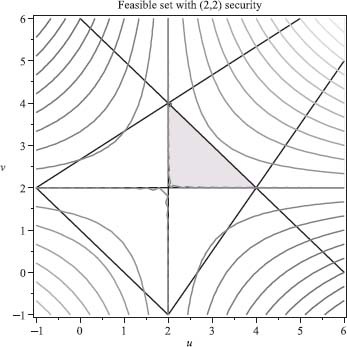
Next, since the Pareto-optimal boundary is u + v = 6, we have mp = −1, b = 6. We calculate value(−mp A − B) and the saddle strategies for that game to get value(A − B) = 2, Xt = (1, 0), Yt = (1, 0).
The threat security point is, therefore, (ut, vt) = (4, 2) with threat strategies Xt = (1, 0) = Yt.
Next, we use the formulas
![]()
with b = 6. The threat solution is ![]() with both players threatening to play row 1, column 1.
with both players threatening to play row 1, column 1.
The KS line for (u*, v*) = (2, 2) is v − 2 = k(u − 2), ![]() or simplified to v = u. This intersects u + v = 6, the Pareto-optimal boundary, at (3, 3). Therefore, (3, 3) is the KS solution.
or simplified to v = u. This intersects u + v = 6, the Pareto-optimal boundary, at (3, 3). Therefore, (3, 3) is the KS solution.
There is no KS line for (u*, v*) = (4, 2) because it is on the edge of the Pareto line.
If we consider the cooperative game, the characteristic function is v(1) = v(2) = 2, v(12) = 6, which gives nucleolus and Shapley value (3, 3) and matches with the solution for the (2, 2) security point.
6.61 The matrices are as follows:
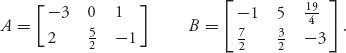
We have ![]() That is our safety point. The Pareto-optimal boundary has three line segments:
That is our safety point. The Pareto-optimal boundary has three line segments:
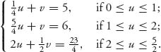
The Nash problem is
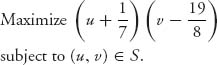
The part of the Pareto-optimal boundary for this problem is the line segment ![]() Using calculus, we find
Using calculus, we find
![]()
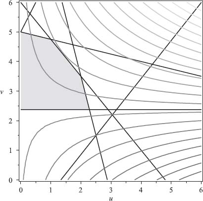
Next, we consider the threat solution. We have to find the threat strategies for all three line segments:
1. ![]() Then
Then ![]() and
and
![]()
and
![]()
Since 5.87 ![]() [0, 1], this is not the threat solution.
[0, 1], this is not the threat solution.
2. ![]() Then
Then ![]() b = 6, and
b = 6, and
![]()
Then
![]()
This is in the range. Let's check the final segment.
3. ![]() In this case
In this case ![]() and
and
![]()
The safety point is then
![]()
Since ![]() this too is not the threat solution.
this too is not the threat solution.
We conclude that the threat solution is ![]() and player 1 threatens to always play the second row; player 2 threatens to use the third column unless they both come to their senses.
and player 1 threatens to always play the second row; player 2 threatens to use the third column unless they both come to their senses.
Finally we determine the KS solution for the safety point ![]()
We have ![]() Then
Then
![]()
is the KS line, and this intersects the Pareto optimal boundary through the segment ![]() at the point
at the point ![]() and that is the KS solution.
and that is the KS solution.
6.63 The spread is 350 − 305 = 45K. If the process ends with at most three stages, player 1 should offer 305 + 0.99 (45) = 349.55. If the process could go on indefinitely, player 1 should offer 305 + 0.5025 (45) = 327.625, because ![]()
6.65.a The Nash problem is
![]()
with (p, w) ![]() S, where
S, where
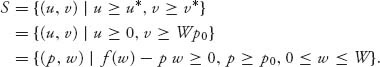
6.65.b Set h(p, w) = (f(w) − p w)(p − p0)w. We have
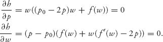
Solving the first equation for p gives
![]()
Substitute this p into the equation hw = 0 to get
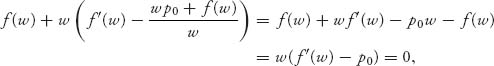
which implies f′(w) = p0.
6.65.c Using the formulas from the previous part, ![]() that implies
that implies ![]() and
and
![]()
6.67 False.
6.69 1. v(![]() ) = 0
) = 0
2. ![]()
3. ![]()
6.71 EI(X*, Y*) ≥ EI(X, Y*), and EII(X*, Y*) ≥ EII(X, Y*) for evey strategy X ![]() Sn and Y
Sn and Y ![]() Sm.
Sm.
6.73 Equality of payoffs says that if (X* = (x1, …, xn), Y*) is a Nash equilibrium and xi > 0, xj > 0 then EI(i, Y*) = EI(j, Y*).
6.75 … if the slope was positive it would mean that both players could increase their payoffs and remain in the feasible set.
Solutions for Chapter 7
7.1 Let’s look at the equilibrium X1 = (1, 0). We need to show that for x ≠ 1, u(1, px + (1 − p)) > u(x, px + (1 − p)) for some px, and for all 0 < p < px. Now u(1, px + (1 − p)) = 1 − p + px, and u(x, px + (1 − p)) = p + x − 3px + 2px2. In order for X1 to be an ESS, we need 1 > 2p(x − 1)2, which implies 0 < p < 1/(2(x − 1)2). So, for 0 ≤ x < 1, we can take px = 1/(2(x − 1)2) and the ESS requirement will be satisfied. Similarly, the equilibrium X2 = (0, 1) can be shown to be an ESS. For ![]() we have
we have
![]()
In order for X3 to be an ESS, we need
![]()
which becomes ![]() for 0 < p < px. This is clearly impossible, so X3 is not an ESS.
for 0 < p < px. This is clearly impossible, so X3 is not an ESS.
7.3 The pure Nash equilibria (X2, Y2), (X3, Y3) are not symmetric and hence cannot be ESSs. We determine whether or not X1 is an ESS.
We calculate for ![]()
![]()
and
![]()
The question is whether (for small enough 0 < p < 1) we have
![]()
Since 98x2 − 28x + 2 = 2(7x − 1)2 > 0 for any ![]() we conclude that
we conclude that ![]() is indeed an ESS. Consequently, in a series of naval battles between the British and French, strong navys will always attack, while weak navys will attack with probability
is indeed an ESS. Consequently, in a series of naval battles between the British and French, strong navys will always attack, while weak navys will attack with probability ![]()
7.5 The Nash equilibria and their payoffs are shown in the following table; they are all symmetric.
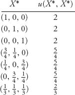
For X* = (1, 0, 0), you can see this is an ESS because it is strict. Consider next ![]() Since
Since ![]() the set of best response strategies is Y = (y, 1 − y, 0). Then u(Y, Y) = 4y2 − 4y + 2 and
the set of best response strategies is Y = (y, 1 − y, 0). Then u(Y, Y) = 4y2 − 4y + 2 and ![]() Since it is not true that u(Y, Y) < u(X*, Y), for all best responses Y ≠ X*, X* is not an ESS.
Since it is not true that u(Y, Y) < u(X*, Y), for all best responses Y ≠ X*, X* is not an ESS.
7.7.a There is a unique Nash, strict and symmetric ESS X* = (0, 1) if a < 0, b > 0, and X* = (1, 0) if b < 0, a > 0.
7.7.b There are three Nash equilibria, all symmetric, Nash equilibria = (1, 0), (0, 1), X, where ![]() Both (1, 0), (0, 1) are strict, (1, 0), (0, 1) are both evolutionary stable. The mixed X is not an ESS since
Both (1, 0), (0, 1) are strict, (1, 0), (0, 1) are both evolutionary stable. The mixed X is not an ESS since
![]()
7.7.c There are two strict asymmetric Nash Equilibria, and one symmetric Nash Equilibrium given by ![]() However, now X is an ESS since
However, now X is an ESS since
![]()
and for every strategy
![]()
so X is an ESS.
7.9.a The replicator equation in simplified form is
![]()
7.9.b The three Nash equilibria are ![]() and the two nonsymmetric Nash points ((0, 1), (1, 0)), and ((1, 0), (0, 1)). So only X1 is a possible ESS. It is not hard to show directly that X1 is an ESS but we can also use the fact from (7.1.9) that if a11 ≠ a21 and a22 ≠ a12, then there must be an ESS. Since the nonsymmetric Nash equilibria cannot be ESSs, the only possibility is X1. Therefore, X1 is an ESS.
and the two nonsymmetric Nash points ((0, 1), (1, 0)), and ((1, 0), (0, 1)). So only X1 is a possible ESS. It is not hard to show directly that X1 is an ESS but we can also use the fact from (7.1.9) that if a11 ≠ a21 and a22 ≠ a12, then there must be an ESS. Since the nonsymmetric Nash equilibria cannot be ESSs, the only possibility is X1. Therefore, X1 is an ESS.
7.9.c From the following figure you can see that ![]() as t → ∞ and conclude that (X1, X1) is an ESS. Verify directly using the stability theorem that it is asymptotically stable.
as t → ∞ and conclude that (X1, X1) is an ESS. Verify directly using the stability theorem that it is asymptotically stable.
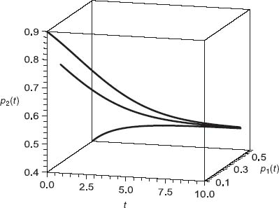
The figure shows trajectories starting from three different initial points. In the three-dimensional figure, you can see that the trajectories remain in the plane p1 + p2 = 1. The Maple commands used to find the stationary solutions, check their stability, and produce the graph are as follows:
> restart:with(DEtools):with(plots):with(LinearAlgebra):
> A:=Matrix([[3, 2], [4, 1]]); X:=< x1, x2>;
> Transpose(X).A.X;
> s:=expand(\%);
> L:=A.X; f:=(x1, x2)->L[1]-s;g:=(x1, x2)->L[2]-s;
> solve({f(x1, x2)=0, g(x1, x2)=0}, [x1, x2]);
> q:=diff(f(x1, x2), x1)+diff(g(x1, x2), x2);
> with(VectorCalculus):Jacobian(<f(x1, x2), g(x1, x2)>, [x1, x2]);
> j:=simplify(\%);
> a1:=subs(x1=1/2, x2=1/2, j);b1:=subs(x1=1/2, x2=1/2, q);
> Determinant(a1);
> DEplot3d({D(p1)(t)=p1(t)*(3*p1(t)+2*p2(t)
                    -3*p1(t)^2-6*p1(t)*p2(t)-p2(t)^2),
            D(p2)(t)=p2(t)*(4*p1(t)+p2(t)
                    -3*p1(t)^2-6*p1(t)*p2(t)-p2(t)^2) },
            {p1(t), p2(t)}, t=0..10,
            [[p1(0)=0.1, p2(0)=0.9], [p1(0)=0.6, p2(0)=.4],
            [p1(0)=1/4, p2(0)=3/4]], scene=[t, p1(t), p2(t)],
            stepsize=.1, linecolor=t);
For the problem, Determinant(a1)=5>0, and b1=-6<0, so the stability Theorem 7.2.3 allows us to conclude that ![]() is asymptotically stable.
is asymptotically stable.
7.11.a The unique Nash equilibrium is ![]() and it is symmetric. We obtain this from the equality of payoffs theorem or Problem 3.25. We calculate using
and it is symmetric. We obtain this from the equality of payoffs theorem or Problem 3.25. We calculate using
![]()
and get ![]() Observe that if we want to use the formula for X* in Problem 3.25, we must use B = AT.
Observe that if we want to use the formula for X* in Problem 3.25, we must use B = AT.
7.11.b We check that with u(X, Y) = X A YT
![]()
for any X ![]() S3. Now we check if u(X*, X) > u(X, X) for all X
S3. Now we check if u(X*, X) > u(X, X) for all X ![]() S3. We have
S3. We have
![]()
The easiest way to check if this is > 0 is to graph the function, or to minimize the function. We’ll do both. First, we have
![]()
and the problem becomes
![]()
We can do this by calculus or with Mathematica. The minimum is 0 attained at ![]() Thus, f(x1, x2) > 0 at any point except at the Nash equilibrium X*. This tells us that X* is indeed an ESS. Here is the graph of f showing it is positive except for the minimum point.
Thus, f(x1, x2) > 0 at any point except at the Nash equilibrium X*. This tells us that X* is indeed an ESS. Here is the graph of f showing it is positive except for the minimum point.
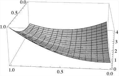
7.11.c The replicator equations are as follows:
![]()
Using p3 = 1 − p1 − p2, and a lot of algebra we get the replicator equations for p1, p2 are as follows:
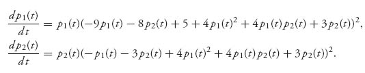
Then ![]() is a stationary solution. To check stability, we use Theorem 7.2.3. These calculations may be done by hand but Mathematica is way easier. Here are the commands to do this:
is a stationary solution. To check stability, we use Theorem 7.2.3. These calculations may be done by hand but Mathematica is way easier. Here are the commands to do this:
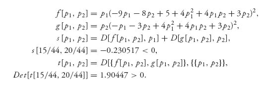
The third line calculates fp1 + g p2, and the fifth line calculates the determinant of the Jacobian matrix given in the fourth line. By the Theorem 7.2.3, we conclude that ![]() is asymptotically stable.
is asymptotically stable.
The remaining stationary solutions are (p1 = 0, p2 = 1), (p1 = 0, p2 = 0), and (p1 = 1, p2 = 0). The convergence to ![]() is shown in the figure.
is shown in the figure.
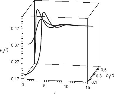
7.13.a ![]() is the unique symmetric Nash equilibrium. But since u(Y, Y) = 0, u(Y, X*) = 0, and u(X*, Y) = 0, it will not be true that u(Y, Y) < u(X*, Y) for all Y that is a best response to X*.
is the unique symmetric Nash equilibrium. But since u(Y, Y) = 0, u(Y, X*) = 0, and u(X*, Y) = 0, it will not be true that u(Y, Y) < u(X*, Y) for all Y that is a best response to X*.
7.13.b It still is true that ![]() is the unique symmetric Nash equilibrium. Now we calculate for any Y = (y1, y2, 1 − y1 − y2).
is the unique symmetric Nash equilibrium. Now we calculate for any Y = (y1, y2, 1 − y1 − y2).
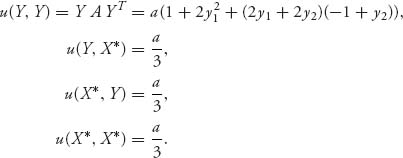
Hence, we are in the condition u(X*, X*) = u(Y, X*), and we have to check if u(X*, Y) > u(Y, Y) for every Y ≠ X*. However,
![]()
is ![]() Thus, it is not true that X* is an ESS.
Thus, it is not true that X* is an ESS.
7.13.c The reduced replicator equations are as follows
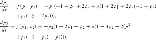
Then
![]()
and ![]() According to Theorem 7.2.3, X* is unstable. This is illustrated in the following figure in the case when a = 0.
According to Theorem 7.2.3, X* is unstable. This is illustrated in the following figure in the case when a = 0.
The case when ![]() is not ESS.
is not ESS.
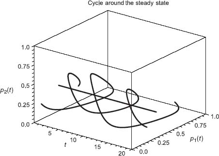
The case when a = 2 is shown in the following figure.
The case a = 2, ![]() is not ESS
is not ESS
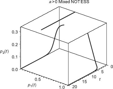
You can see that unless you start exactly at X*, the trajectories converge to one of the pure Nash equilibria.
7.15 The difference between this problem and the matrix in Problem 7.13.b is that we are taking the negative of the matrix. We consider
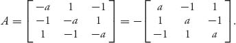
It still is true that ![]() is the unique symmetric Nash equilibrium. We see this by calculating
is the unique symmetric Nash equilibrium. We see this by calculating
![]()
Now we calculate for any Y = (y1, y2, 1 − y1 − y2)
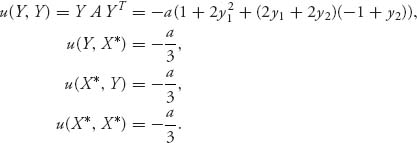
Again the condition u(X*, X*) = u(Y, X*) holds and we have to check if u(X*, Y) > u(Y, Y) for every Y ≠ X*. We consider,
![]()
over all strategies Y and calculate that this minimum is zero, attained only when Y = X*. Thus, in this case X* is an ESS. Here is the figure for the replicator dynamics.
When diagonal < 0, ![]() is ESS
is ESS