
Special Topics B: Applications to Accelerated Testing
B.1 Introduction
In this section we provide some examples of how to use the acceleration models detailed in Chapter 4 and elsewhere in this book.
Accelerated testing is the cornerstone of reliability testing by companies all over the world. There are a number of reliability conferences where the majority of the papers pertain to the subject of accelerated testing done on products in industry. The reader is referred to two of the most popular conferences called Accelerated Stress Testing and Reliability (ASTR) conference and Reliability and Maintainability Symposium (RAMS). In many industries, “Failure is not an Option”; this is in fact a slogan often coined by NASA. It fact NASA engineers make up the largest group of attendees at these conference every year. In terms of thermodynamic reliability, entropy damage in systems is a big concern and what better way to look for potential entropy problems than by doing accelerated testing. Tests are typically divided up into five main categories related to the popular stresses used in industry: high temperature; thermal cycle; temperature–humidity; salt fog; and shock and vibrations corrosion testing. These tests are exemplified in Figure B.1.

Figure B.1 Main accelerated stresses and associated common failure issues
We note that high-temperature accelerated testing is often used to look at issues of intermetallics and diffusion as well as thermomechanical failure mechanisms (that can include wire bond integrity, Kirkendall voiding, ohmic contact issues, electromigration) and semiconductor junction issues such as metal oxide semiconductor (MOS) gate wear-out and so forth. Heat is often an enemy as it increases the devices entropy. As in semiconductor testing, devices are often biased to include the high-temperature junction rise.
Temperature cycle accelerated testing is often used to look at expansion–contraction temperature coefficient of thermal expansion (TCE) mismatch issues. For example, one of the most common issues in electronic circuit boards is the TCE mismatch between large solder components and the printed circuit board. Ceramic ball grid arrays (BGAs) for example in contact to a common FR-4 board can have a TCE mismatch of 11.5 ppm/°C. Such mismatches cause stress which, in combination with a large-size BGA, can cause early life failure.
Temperature–humidity–bias testing is also a very common accelerated test. Harsh tropic environments with high humidity present challenges for electronic components in the field. This test looks for moisture-related failure mechanisms such as silver migration from silver-filled epoxies, electrical breakdown, plastic IC moisture ingress leading to complex solder reflow expansion package cracking issues, and so forth.
Shock and/or vibration are important tests as products in the field experience minimally transportation vibration in shipping. As well some products are in harsh shock and vibration environments such as automotives and aircraft. Typically, shock testing is not accelerated as it can often be done on a repetitive electrodynamic shaker where numerous shocks can be applied to equate to the actual product life. However, vibration testing needs to be accelerated.
Finally, corrosion testing can be important. It is estimated that corrosion problems have annually cost up to $350 billion in the US alone, of which 40% could likely be prevented. Accelerated testing (such as salt fog or humidity testing) can play a big part in understanding potential product corrosion issues.
B.1.1 Reliability and Accelerated Testing Software to Aid the Reader
It is helpful to use software in understanding the reliability and accelerated testing analysis described here and in Special Topics A. Free reliability statistics and accelerated testing software is available to aid the reader at the author’s website, www.dfrsoft.com, to try for all the examples in Special Topics A and B [1]. This chapter provides reference to the module and row number that the reader can go to in the software to follow with the examples, for example (dfrsoft, module 2, row 13). The software is in friendly Excel format with reference modules (see menu) that includes help in the following areas: reliability conversion; reliability plotting (Weibull, lognormal, …); system reliability; distributions; field returns; acceleration factors; test plans; environmental profiling; reliability growth; reliability predictions; parametric reliability; availability and sparing; derating; physics of failure; Cpk analysis; lot sampling; SPC; thermal analysis; shock and vibration; corrosion; and design of experiment.
Testing for a product can often include multiple combinations of these tests [2, 3]. Figure B.2 illustrates a common test flow that one might use for multiple testing on a product (dfrsoft, module 15, row 207 [1]). We see that testing exposes the product flow to all stresses. Depending on the target failure modes if known, one can focus more on one stress than the others. Typically, the key stress may not be known. Most of the time, qualification testing is done using accelerated testing at a certain level of confidence. This allows a target reliability goal to be proven for the qualification test to within a certain upper confidence level of the failure rate. This will be discussed in the next sections (also see Section B.6.1).

Figure B.2 Common accelerated qualification test plan used in industry [1]
B.1.2 Using the Arrhenius Acceleration Model for Temperature
Often, it is assumed that the dominant thermally accelerated failure mechanisms will follow the classical Arrhenius relationship described by Equation (5.20). The basic acceleration factor model is repeated here for convenience:

where ![]() is Boltzmann’s constant. Boltzmann originally proposed a similar relation as a probability distribution (see Section 6.3). There are a number of ways this model is used. In degradation, we can think of it in terms of defect activation. In this view, there is a certain probability of a defect surmounting the free energy barrier (see Figure 6.1). When enough defects are thermally activated over time, catastrophic failure results, the system’s entropy is maximum (maximum disorder) and aging stops as the system is in its lowest free energy state, a state of final equilibrium. Note that since kB has units of degrees Kelvin, so must the temperatures T1 and T2. Although we found this for corrosion, this relationship is relevant to many thermally activated processes. The rate can be written as
is Boltzmann’s constant. Boltzmann originally proposed a similar relation as a probability distribution (see Section 6.3). There are a number of ways this model is used. In degradation, we can think of it in terms of defect activation. In this view, there is a certain probability of a defect surmounting the free energy barrier (see Figure 6.1). When enough defects are thermally activated over time, catastrophic failure results, the system’s entropy is maximum (maximum disorder) and aging stops as the system is in its lowest free energy state, a state of final equilibrium. Note that since kB has units of degrees Kelvin, so must the temperatures T1 and T2. Although we found this for corrosion, this relationship is relevant to many thermally activated processes. The rate can be written as

where ν is a rate constant. We note that Ea can be thought of as the free energy barrier height. The barrier height is a property of the system’s free energy related to the type of material (see Chapter 6 for more details). The expression is often written in linear Y = ax + b form so that the time to failure can be plotted for regression analysis as:

where the constant is simply ln(1/ν).
Each failure mechanism that is thermally activated has associated with it an activation energy Ea. A number of different failure mechanisms and values for Ea can be found in Table 6.1, with general ranges often cited in the literature. We note that the higher the temperature, the more likely is the probability of a defect being excited and jumping over the free energy barrier. In a sense the barrier is a relative minimum of the free energy (see Figure 6.1), not the true minimum. However, when enough defects surmount the barrier and catastrophic failure occurs, the free energy is then at its true minimum.
In practice, when trying to estimate acceleration factors without knowing the activation energy value for each potential failure mechanism, a conservative value of Ea is used. For example, 0.7 eV is typical for IC failure mechanisms and appears to be somewhat of an industry standard when conservatively estimating test times (see Table 6.1).
B.1.2.1 Example B.1: Using the Arrhenius Acceleration Model
Consider a semiconductor device with a thermal resistance of 20°C/W (junction to ambient). The device is operated at 0.5 W. It is typically operated at 30°C and is tested at 100°C. What is the required test time to simulate 10 years of life in reliability testing? Assume an activation energy of 0.7 eV for the failure mechanism.
- Analysis: First we find the power dissipated in the device at 0.5 W × 20°C/W. The junction rise is 10°C over ambient.
Then the field use condition is Tuse = 10°C + 30°C = 40°C = 273.15 + 40 = 313.15 K.
The stress temperature condition is Tstress = 10°C + 100°C = +110°C = 383.15 K.
From Equation (B.1), the acceleration factor is (dfrsoft, module 7, row 13 [1])
AFT = exp {(0.7 eV/8.6173 × 10−5 eV/K) × [1/(313.15) − 1/(383.15) K]} = 114.The test time to simulate 10 years of life (87 600 h) is
Test time = Lifetime/AFT = 87 600/114 = 768 h.In the above we assumed an activation energy of 0.7 eV. One might ask: what if we wish to find this value? In process reliability for example, one can test multiple devices in groups at high temperature. Then the mean time to failure (MTTF) for each temperature group is assessed and the result can be plotted according to Equation (B.3) to find the activation energy for the failure mechanism associated with the test item. If for example only two temperatures are used, then we can solve Equation (B.1) directly for the activation energy which yields:
(B.4)
and we substitute the numbers. A more instructive problem is given below.
B.1.3 Example B.2: Estimating the Activation Energy
A process reliability study was performed on semiconductors at six different temperatures. The results yielded the following MTTFs.
Find the activation energy for the process and estimate the MTTF at a field use condition of 50°C.
Using (dfrsoft, module 7, row 99 [1]) Equation (B.3) we can plot ln(MTTF) against 1/T. Then using a linear regression analysis, we can find the slope of the line. The slope should yield a value of Ea/kB. The graphical result is presented in Figure B.3 (see also Table B.1; dfrsoft, module 7, row 139 [1]).

Figure B.3 Arrhenius plot of data given in Table B.1
Courtesy: DfR Software company
Table B.1 MTTF observed
| Temperature (°C) | MTTF |
| 140 | 2000 |
| 150 | 1400 |
| 160 | 850 |
| 170 | 550 |
| 185 | 300 |
| 220 | 90 |
The slope yields an activation energy of 0.692 eV. Using this we can project the MTTF at 50°C, which will yield an MTTF of 464 909 h.
B.1.4 Example B.3: Estimating Mean Time to Failure from Life Test
In Section B.1.2.1 what is the upper 90% confidence bound on the failure rate if 25 devices are tested and only 1 failure is observed? We use the method adopted in Section A.8. The chi-squared value is:
The value χ2(0.9, 4) = 7.78 may be found in statistical tables. The device hours is 25 × 768 h × 114 = 2 188 800 device hours. Assuming a constant failure rate, the 90% upper bound on the failure rate is (dfrsoft, module 8, row 11, col. m [1]):
The MTTF is ![]() , which is a lower bound 90% confidence limit on the MTTF. Note the point estimate is 0.46 FMH = 1 failure/2 188 800 device hours.
, which is a lower bound 90% confidence limit on the MTTF. Note the point estimate is 0.46 FMH = 1 failure/2 188 800 device hours.
B.2 Power Law Acceleration Factors
Chapter 4 presented numerous acceleration factors; we can quickly summarize a few here for convenience. The acceleration factor found for creep in Equation (4.16) was

and its linear relationship for the time to failure was noted in Equation (4.18) as
We noted that the acceleration factor for wear, while not a power function, can be thought of as a power law with a power factor of 1. This was given in Equation (4.23) as

and the linear time to failure dependence is, from Equation (4.25):
The temperature cycle acceleration factor was given found in Equation (4.30) as
and its relationship for the time to failure is similar to that for creep, as given in Equation (4.32):
The acceleration factor for vibration was obtained in Equation (4.39) as

We note that we could substitute for the Grms level the power spectral density (PSD) level, Wpsd with an exponent −b/2 in Equation (4.46). The cycles to failure at any stress level gave the form of the S–N curves in Equation (4.42) as
However, we can linearize this as
where D is of course ln(C).
What we would like to point out is that the times to failure all have a common linearized form Y = aX + B as
with an arbitrary stress acceleration factor given by

B.2.1 Example B.4: Generalized Power Law Acceleration Factors
We would like to present an example of using the power law form in Equations (B.5–B.13) by specifically using the form of Equations (B.14) and (B.15) for an unknown mechanical stress.
A machine provides an unusual stress type that is not well known. It is not covered by either of Equations (B.14) and (B.15), but we suspect as with most of the stress-related time to failure equations (except for the Arrhenius equation) that it will be governed by a power law. Table B.2 lists the failure times using a machine with knob settings of stress levels.
Table B.2 Machine stress MTTF observed
| Machine stress level knob setting | Machine stress MTTF (h) |
| 3 | 175 |
| 4 | 80 |
| 5 | 50 |
| 6 | 30 |
| 7 | 20 |
Assess the test results to determine if the machine’s stress is causing a time to failure that has a power law form. Extrapolate the result to a knob stress level of 1.5.
Using the generalized Equation (B.14), we plot ln(MTTF) against ln(stress) as shown on the log–log plot. Using a linear regression analysis, we find the slope of the line. The result is shown in Figure B.4. Indeed, the straight line linear regression fit in the figure indicates that the power law (Equation (B.14)) is a good fit (dfrsoft, module 7, row 157 [1]).

Figure B.4 MTTF stress plot of data given in Table B.2.
Courtesy: DfR Software company
The slope yields a K value of –2.5. We can see that it is also an inverse relationship by the negative slope. The intercept is 2793.7. Using these results we can project the MTTF to a 1.5 stress level; this will yield an MTTF of about 1000 h where MTTF(1.5) = 2793.7 (1.5)–2.5 (dfrsoft, module 7, row 185 [1]).
B.3 Temperature–Humidity Life Test Model
The analysis for corrosion yielded a temperature–humidity acceleration factor given in Equation (5.34) as
The temperature acceleration factor AFT and the humidity acceleration factor AFH were obtained in Equation (5.35), given by

We note that the acceleration factor for humidity is interestingly enough a power law function. This expression is widely used in industry today for humidity testing to make an assessment of the accelerated time that occurs when items are put into a temperature–humidity chamber. The most common test used in the industry is a 1000 h test at 85°C and 85% relative humidity. This model in the industry is a 1986 Peck model [4]. In the Peck model from his data on corrosion testing of microelectronics in 1986, he found M = 2.66 and Ea = 0.7. Often these numbers are used in the literature. The fact that the overall acceleration factor is a product of two acceleration factors indicates independence of the stresses. It also provides a fairly large acceleration factor as we will note in the next example. Although 1000 h of testing is quite common, the model suggest that only 133 h is needed to accelerate to 10 years as we will show in the next example. Note that in normal chambers, the temperature is limited to less than 100°C, the boiling point. However, highly accelerated stress test (HAST) pressure chambers are often used to allow a test temperature higher than 100°C, typically 110–130°C with humidity usually set at 85%.
B.3.1 Temperature–Humidity Bias and Local Relative Humidity
The temperature–humidity test is usually performed in microelectronics with products under minimum bias. This is because a number of failure mechanisms are driven by bias, such as silver migration, corrosion, dielectric breakdown, and so forth. That being said, minimum bias is usually tested at product specification. The minimal bias is applied so that the local relative humidity will minimally be reduced by components that generate heat. According to JESD22-A100D (see http://www.jedec.org), if the junction temperature rise of a component exceeds 10°C then it recommends that cycle bias will be a more severe test than continual bias for such parts. Usually cycle bias during humidity testing is typically performed at a rate of 12 h on and 12 h off. It is helpful to estimate the local relative humidity when calculating the acceleration factor for a particular part. This can actually be calculated using the method given in JEDEC Specification 94A (see http://www.jedec.org) or using appropriate software [1].
B.3.1.1 Example B.5: Using the Temperature–Humidity Model
Consider a temperature–humidity test at 85°C and 85% relative humidity (%RH). For a test running for 130 h, estimate the equivalent field time if the field conditions are 25°C and 40% RH using the Peck model parameters. Also assess this when a component has a junction rise of 20°C.
Part 1
Using the Arrhenius model with ![]() and Ttest = 85°C = 358.15 K, and Tuse = 25°C = 298.15 K, we find
and Ttest = 85°C = 358.15 K, and Tuse = 25°C = 298.15 K, we find
The humidity acceleration factor is then simply 7.43. Then the overall acceleration factor is (dfrsoft, module 7, row 28 [1]):
For a 130 h test this equates to 713 × 130 = 10.6 years equivalency in the field.
Part 2
If the junction temperature for another part is 20°C higher, then Ttest = 85°C + 20°C = 105°C = 378.15 K and Tuse = 25°C + 20°C = 318.15 K. The acceleration factor is then
To find the acceleration factor for humidity, we must now use the method JEDEC Specification 94 (see www.jedec.org). We leave the exercise mostly to the reader. However, we find that the local relative humidity on an 85% RH test at 105°C is 40% RH (dfrsoft, module 1, row 175 [1]). The same exercise can be done for the local relative humidity if the ambient temperature is 25°C and 40% RH. Then if the junction rise yields a junction temperature of 45°C, we find the local relative humidity at the die is only 13% RH. Then the humidity acceleration factor is
The relative humidity acceleration factor is then (dfrsoft, module 7, row 28 [1]):
For a 130 h test this equates to 1143 × 130 = 17 years equivalency in the field. This is a bit interesting. Even though the temperature acceleration factor is reduced, the humidity acceleration factor actually increased as the local relative humidity in the field is only 13% due to the junction rise for an ambient at 40% RH.
B.4 Temperature Cycle Testing
The temperature cycle given in Equation (B.9) helps to access the test time equivalency to cyclic field use conditions. The key things to be careful about when using the model are as follows in the case of solder joint issues.
- What are the numbers of cycles per day in the field?
- What is the best estimate for ΔT in the field and for the test?
- Do we need to worry about the Arrhenius factor and the frequency effect?
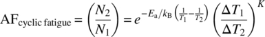
For solder fatigue, an alternate model was proposed by Norris and Lanzberg [5]. This model is Equation (B.9) with the frequency effect factor added for the amount of cycles per unit time observed:

The use of this model for the frequency effect is as follows. For lead-free SAC (Sn/Ag/Cu) solder, if the maximum upper cycle temperature is greater than 1/2 of the melting temperature (c. 216°C/2 = 108°C) and if the cyclic frequency is longer that about 17 min, the frequency effect is said to come into play. Below this temperature there is little effect on fatigue (we ignore the frequency effect) as creep plays less of a role.
For non-solder fatigue (where the frequency effect is not used), most users ignore the temperature Arrhenius factor which we found should be added in Chapter 4.
B.4.1 Example B.6: Using the Temperature Cycle Model
A temperature-cycle test is performed for 200 cycles from –25°C to +125°C. How many cycles is this in the field at 1 or 2 cycles a day for delta use of 0–35°C? Assume a conservative temperature cycle exponent of 2.0.
Analysis: The temperature cycle ΔT factor is (dfrsoft, module 7, row 42 [1])
 .
. For the Arrhenius part we use the upper temperature for field and use condition of 35°C and 125°C. The activation energy commonly used for solder fatigue is 0.123 eV. We have not really specified what we are actually testing. Often we may not know the actual Arrhenius activation energy. If we are concerned with creep and fatigue as in Equation (B.18), then perhaps this would be a good number. Using it we find the Arrhenius part is 2.85 (dfrsoft, module 7, row 81 [1]).
Then we can compare with and without the Arrhenius factor. Without the Arrhenius factor the field years = 18.4 × 200/365 = 10 years and with it the field years = 28.5 years.
Now if the product was exposed to 2 cycles per day in the field, this would be equivalent to 14.25 years.
B.5 Vibration Acceleration
There are two main types of vibration tests where one simulates field use conditions; these are sine or random vibration.
Sine vibration testing has products exposed to sinusoidal vibrations as for type shown in Figure B.5. Sine vibration is usually specified in terms of G where the unit G denotes acceleration of gravity (9.8 m/s2). If for example a system is in free fall, then this is 1 G. In sine vibration testing, products are mounted on an electrodynamic shaker and often certain specifications pertain. For example, MIL-STD 810E is one of the most common specifications. There are two main types of sine tests: these are a sine sweep and the other is a resonance dwell. Often one use sine sweep to look for resonances.

Figure B.5 Sine vibration amplitude over time example
Typically, the motivation for doing sine testing is to simulate field use conditions that are sinusoidal-like. Highly periodic sine-like vibrations occur for say electric motors, helicopter periodic blade motion, or other similar propeller-type aircraft. Some vibration types such as helicopters are mixed and require both sine and random vibration testing. This is often termed sine on random (dfrsoft, module 5, row 24 [1]).
Random vibration testing is usually performed to simulate field use condition. As the name suggests, the vibration is truly random. This is displayed in Figure B.6. Unlike sine vibration where the amplitude is known with a specific G-level, random amplitude happens with a probability of occurrence. A common type of random vibration often observed in the field is Gaussian. Table B.3 displays the probabilities for Gaussian vibration. For example, the amplitudes will be above 3σ about 0.27% of the time and above 4σ just 0.006% of the time. Note Gaussian vibration has a mean of zero so σ (which is the Grms content for Gaussian vibration) is the actual amplitude in terms of Grms. For a random vibration of 60 s the amount of the time at which the amplitude will be greater than 1σ is 60 s × 0.3173 = 18.22 s; the amount of time at which the amplitude will be less than 1σ is 60 s × 0.683 = 41 s.

Figure B.6 Random vibration amplitude time series example
Table B.3 Gaussian probabilities (%)
| 1σ | 2σ | 3σ | 4σ |
| Two-sided probability | |||
| 68.27 | 95.45 | 99.73 | 99.99 |
| Percent above | |||
| 31.73 | 4.55 | 0.27 | 0.006 |
Another aspect of random vibration is the concept of going from the time series spectrum in Figure B.6 and performing a Fourier transform to obtain the frequency spectrum graph shown in Figure B.7 (dfrsoft, module 25, row 71 [1]). The frequency spectrum plot is termed the PSD plot. This graph looks a lot easier to interpret than the time domain plot; test specifications are often provided in the frequency domain for this reason. The area under the PSD curve is the Grms content. When doing accelerated testing one can use either the PSD peak levels or the Grms content. The equations are almost the same. For the interested reader this is the difference between using Equations (4.39) and (4.45), where the exponent is divided by two resulting from finding the area under the PSD curve. For example, the value of b ≈ 5 is commonly used for electronic boards. However, a conservative value for the fatigue parameter b is about 8 (e.g., Mb = 4). MIL STD 810E (method 514.4−46) recommends b = 8 for random loading.
Figure B.7 PSD of the random vibration time series in Figure B.6
Random vibration is also performed on an electrodynamic shaker which is capable of accelerated testing on products requiring either sine or random vibration. Often specifications from MIL STD 810 are used. Alternately, one can design their own test to simulate field conditions.
B.5.1 Example B.7: Accelerated Testing Using Sine and Random Vibration
An accelerated test is required to simulate 10 years of life for sine testing at resonance occurring at 100 Hz. The accelerated test is specified for 4 G of sine vibration where in the field the product is only exposed to a 1.5 G level at a resonance of about 2% of the time. Use a sine vibration exponent of 5.
Estimate the time to simulate 10 years of life for an assembly that is to be tested at a PSD level of 0.12 G2/Hz from 0 to 2000 Hz. It is estimated that the assembly will undergo a worst case of 1% exposure of 0.03 G2/Hz over this bandwidth. Use MIL STD 810 Mb = 8.
Sine Vibration Analysis
The sine vibration acceleration factor is that of Equation (4.39), also given in Section B.2.4 is

The test for 10 years in the field is about 10 × 8760 × 2%/335.5 = 5.22 h (dfrsoft, module 25, row 158, col B [1]).
Random Vibration Analysis
The random vibration acceleration factor is from Equation (4.45):

The test for 10 years in the field is about 10 × 8760 × 1%/256 = 3.4 h (dfrsoft, module 25, row 158, col C [1]).
B.6 Multiple-Stress Accelerated Test Plans for Demonstrating Reliability
Multiple test demonstration testing of the type shown in Figure B.2 is set up to demonstrate an overall failure rate with a certain level of confidence that helps determine the sample size for each test. The overall goal is to demonstrate a certain failure rate over multiple stresses that the product might be subjected to in the field. The most common stress that are tested for microelectronics is high-temperature operating bias (see Section B.1), humidity–temperature bias (see Section B.3), and temperature cycle (see Section B.4). Further, if we are concerned with vibration (Section B.5) than this must be included as well. One of the key obstacles in designing such a test is to allocate the failure rate among the tests. For example, if the desired overall failure rate is say 0.6 FMH, than one possible scenario is to allocate a portion of the failure rate evenly among the tests; in this case that would be 0.2 FMH. Another possible scenario is to optimize the sample size (see example below) among the three tests given constraints on the failure rate and the total sample size. The following example illustrates these methods.
B.6.1 Example B.8: Designing Multi-Accelerated Tests Plans: Failure-Free
An example of equal-failure-rate test allocation is provided in Table B.4. The three stress environments that a product is exposed to are accelerated to demonstrate a failure rate of 0.6 FMH. Using the method in Section B.1.4, one can verify these numbers. The reader may wish to check the values in the table as an exercise (dfrsoft, module 8, row 28, col C, and row 41, col. B [1]). The test constraints are as follows.
- Total failure allowed = 0;
- Confidence level = 90%;
- Failure rate objective = 0.6 FMH;
- High-temperature operating life (HTOL): 1000 h, Tuse = 50°C, Tstress = 125°C, Ea = 0.7 eV;
- Temperature cycle (TC): 200 cycles, ΔTuse = 30°C, ΔTstress = 150°C, exponent 2;
- Temperature–humidity bias (THB): 1000 h, RHuse = 40%, RHstress = 85%, Tuse = 35°C, Tstress = 85°C.
Table B.4 Multiple stress accelerated test to demonstrate 0.6 FMH
| Stress | Chapter example number | Acceleration factor | Test time | FMH | Minimum sample size |
| HTOL | B.1 | 114 | 1000 h | 0.2 | 79 |
| THB | B.5 | 295 | 1000 h | 0.2 | 39 |
| TC | B.6 | 25 | 200 cycles | 0.2 | 96 |
| Total | 0.6 | 236 |
Courtesy: DfR Software company.
Table B.5 below provides another example where equal allocations are not used but we instead seek to optimize for a minimum sample size among the three tests given the same test conditions and constraint of 0.6 FMH objective. As an exercise, the reader may wish to check the optimized results in the table (dfrsoft, module 8, row 28, col C, and row 39, col. L [1]). Comparing Tables B.4 and B.5 we see the optimized results saved about 10 devices.
- Total failure allowed = 0;
- Confidence level = 90%;
- Estimate life each test greater than 10 years;
- Failure rate objective = 0.6 FMH;
- HTOL 1000 h, Tuse = 50°C, Tstress = 125°C, Ea = 0.7 eV;
- TC 200 cycles, ΔTuse = 30°C, ΔTstress = 150°C, exponent 2;
- THB: 1000 h, RHuse = 40%, RHstress = 85%, Tuse = 35°C, Tstress = 85°C.
Table B.5 Optimized multiple stress accelerated test for 0.6 FMH
| Stress | Example number | Acceleration factor | Test time | FMH | Minimum sample size |
| HTOL | B.1 | 114 | 1000 h | 0.233 | 87 |
| THB | B.5 | 295 | 1000 h | 0.144 | 54 |
| TC | B.6 | 25 | 200 cycles | 0.226 | 85 |
| Total | 0.6 | 226 | |||
Courtesy: DfR Software company.
B.7 Cumulative Accelerated Stress Test (CAST) Goals and Equations Usage in Environmental Profiling
In Section 4.4 we described cumulative accelerated stress test (CAST) goals, listed in Table 4.3. To illustrate this for accelerated testing, one needs to estimate the field use conditions. Often, stresses in the field vary over time. For example, a product during a year in the field might be temperature-profiled over say 1 year as indicated in Table B.5.
When this occurs, what stress temperature do we use for an accelerated test and how do we plan it? To this end we now provide an example.
B.7.1 Example B.9: Cumulative Accelerated Stress Test (CAST) Goals and Equation in Environmental Profiling
Consider the 1 year profile in Table B.5 worked out prior to an accelerated test. The reliability engineer needs to figure out a CAST goal for the accelerated test equivalent to infant mortality of 1 year and a life test goal for 10 years. He now uses the temperature CAST goal equation in Table 4.3 that allows him to do so, which is
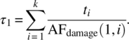
First he defines τ1 as 1 year infant mortality time. Then he starts by estimating a reference stress, let’s try 50°C for AF(1, i). Next he uses the Arrhenius acceleration factor with an activation energy of 0.7 eV for the above equation. With this he simply plugs in the values in Table B.5 to come up with the actual results for τ1 which is equivalent to 8474 h at 50°C. The reader should verify this time (dfrsoft, module 9, row 8, col A, [1]). He can then iterate and refine the reference stress; the actual temperature in this case is very close and is 49.57°C for exactly 1 year. The results of the above equation are shown in Table B.6. For example, dividing the acceleration factor AF (30°C, 49.57°C) = 5.08, shown in column 4, into 2190 gives 431 hours equivalent, as show in column 5. That is, if our environment is profiled at 49.57°C and we did a test at 30°C for 2190 hours, it would equate to 431 hours at 49.57°C. We continue this and note that the sum in column 5 is indeed 1 year equivalent. That is, only this unique profiled temperature equates to 1 year. The reader should verify this temperature. We wanted to simplify the explanation so we used this iterative method.
Table B.6 Profile of a product’s temperature exposure per year
| Temperature | Time/year | Percent of time (%) | AF to 49.57°C | Profiled time at 49.57°C |
| 30 | 2190 | 25 | 5.08 | 431 |
| 40 | 2628 | 30 | 2.16 | 1219 |
| 50 | 2190 | 25 | 0.97 | 2258 |
| 60 | 1314 | 15 | 0.46 | 2891 |
| 70 | 438 | 5 | 0.22 | 1962 |
| Sum | 8760 | 100 | 8760 |
Next the engineer wants to design a 10 year life test. We can simply multiply up the profile in Table B.5 to a 10 year CAST goal and the results will yield the same reference temperature requirement of 49.57°C. With this CAST goal, we can estimate the device hours needed in an accelerated 10 year life test at any reasonable test temperature to achieve enough device hours to verify the 10 year goal relative to the reference temperature of 49.57°C. For example, using the chi-squared method in Section A.8, we have for an accelerated test at 120°C

This is then subject to the restriction that AF × test time = 10 years. We now can trade off between the sample size n and the failure rate λ objective we might need given a certain level of confidence γ and allowed failures y (usually 0 or 1; see Table B.6).
References
- [1] Author’s software, download at http://www.dfrsoft.com (see Section A.1.1 for details) to follow along with examples.
- [2] O’Connor, P. and Kleyner, A. (2012) Practical Reliability Engineering, 5th edn, John Wiley & Sons, Ltd, Chichester.
- [3] Feinberg, A., Crow, D. (eds) Design for Reliability, M/A-COM 2000, CRC Press, Boca Raton, 2001.
- [4] Peck, D.S. Comprehensive model for humidity testing correlation. In Proceedings of the 24th IEEE International Reliability Physics Symposium, April 1986, Anaheim, CA, pp. 44–50.
- [5] Norris, K.C. and Landzberg, A.H. (1969) Reliability of controlled collapse interconnections. IBM Journal of Research and Development, 13 (3), 266–71.