
1
Equilibrium Thermodynamic Degradation Science
1.1 Introduction to a New Science
Thermodynamic degradation science is a new and exciting discipline. Reviewing the literature, one might note that thermodynamics is underutilized for this area. You may wonder why we need another approach. The answer is: in many cases you do not. However, the depth and pace of understanding physics of failure phenomenon, and the simplified methods it offers for such problems, is greatly improved because thermodynamics offers an energy approach. Further, systems are sometimes complex and made up of many components. How do we describe the aging of a complex system? Here is another possibility where thermodynamics, an energy approach, can be invaluable. We will also see that assessing thermodynamic degradation can be very helpful in quantifying the life of different devices, their aging laws, understanding of their failure mechanisms and help in reliability accelerated test planning [1–4]. One can envision that degradation is associated with some sort of device damage that has occurred. In terms of thermodynamics, degradation is about order versus disorder in the system of interest. Therefore, often we will use the term thermodynamic damage which is associated with disorder and degradation. One clear advantage to this method is that:
thermodynamics is an energy approach, often making it easier to track damage due to disorder and the physics of failure of aging processes.
More importantly, thermodynamics is a natural candidate to use for understanding system aging.
Here the term “system” can be a device, a complex assembly, a component, or an area of interest set apart for study.
Although most people who study thermodynamics are familiar with its second law, not many think of it as a good explanation of why a system degrades over time. We can manipulate a phrasing of the second law of thermodynamics to clarify our point [1, 4].
Second law in terms of system thermodynamic damage: the spontaneous irreversible damage processes that take place in a system interacting with its environment will do so in order to go towards thermodynamic equilibrium with its environment.
There are many phrasings of the second law. This phrasing describes aging, and we use it in this chapter as the second law in terms of thermodynamics damage occurring in systems as they age. We provide some examples in Chapter 2 (see Sections 2.10 and 2.11) of this statement in regards to aging to help clarify this.
When we state that degradation is irreversible, we mean either non-repairable damage or that we cannot reverse the degradation without at the same time employing some new energetic process to do so. We see there is a strong parallel consequence of the second law of thermodynamics associated with spontaneous degradation processes.
The science presents us with a gift, for its second law actually explains the aging processes [1, 4].
We are therefore compelled to look towards this science to help us in our study of system degradation. Currently the field of physics of failure includes a lot of thermodynamic-type explanations. Currently however, the application of thermodynamics to the field of device degradation is not fully mature. Its first and second laws can be difficult to apply to complex aging problems. However, we anticipate that a thermodynamic approach to aging will be invaluable and provide new and useful tools.
1.2 Categorizing Physics of Failure Mechanisms
When we talk about system damage, we should not lose sight of the fact that that we are using it as an applicable science for physics of failure. To this end, we would like to keep our sights on this goal. Thermodynamic reliability is a term that can apply to thermodynamic degradation physics of a device after it is taken out of the box and subjected to its use under stressful environmental conditions. We can categorize degradation into categories [1, 2] as follows.
The irreversible mechanisms of interest that cause aging are categorized into four main categories of:
forced processes;
activation;
diffusion; and
combinations of these processes yielding complex aging.
These are the key aging mechanisms typically of interest and discussed in this book. Aging depends often on the rate-controlling process. Any one of these three processes may dominate depending on the failure mode. Alternately, the aging rate of each process may be on the same time scale, making all such mechanisms equally important. Figure 1.1 is a conceptualized overview of these processes and related physics of failure mechanisms.

Figure 1.1 Conceptualized aging rates for physics-of-failure mechanisms
In this chapter, we will start by introducing some of the parallels of thermodynamics that can help in our understanding of physics of degradation problems. Here fundamental concepts will be introduced to build a basic framework to aid the reader in understanding the science of thermodynamic damage in physics of failure applications.
1.3 Entropy Damage Concept
When building a semiconductor component, manufacturing a steel beam, or simply inflating a bicycle tire, a system is created which interacts with its environment. Left to itself, the interaction between the system and environment degrade the system of interest in accordance with our second law phrasing of device degradation. Degradation is driven by this tendency of the system/device to come into thermodynamic equilibrium with its environment. The total order of the system plus its environment tends to decrease. Here “order” refers to how matter is organized, for example disorder starts to occur when: the air in the bicycle tire starts to diffuse through the rubber wall; impurities from the environment diffuse into otherwise pure semiconductors; internal manufacturing stresses cause dislocations to move into the semiconductor material; or iron alloy steel beams start to corrode as oxygen atoms from the atmospheric environment diffuse into the steel. In all of these cases, the spontaneous processes creating disorder are irreversible. For example, the air is not expected to go back into the bicycle tire; the semiconductor will not spontaneously purify; and the steel beam will only build up more and more rust. The original order created in a manufactured product diminishes in a random manner, and becomes measurable in our macroscopic world.
Associated with the increase in total disorder or entropy is a loss of ability to perform useful work. The total energy has not been lost but degraded. The total energy of the system plus the environment is conserved during the process when total thermodynamic equilibrium is approached. The entropy of the aging process is associated with that portion of matter that has become disorganized and is affecting the ability of our device to do useful work. For the bicycle tire example, prior to aging the system energy was in a highly organized state. After aging, the energy of the gas molecules (which were inside the bicycle tire) is now randomly distributed in the environment. These molecules cannot easily perform organized work; the steel beam, when corroded into rust, has lost its strength. These typical second-law examples describe the irreversible processes that cause aging.
More precisely:
if entropy damage has not increased, then the system has not aged.
Sometimes it will be helpful to separately talk about entropy in two separate categories.
Entropy damage causes system damage, as compared to an entropy term we refer to as non-damage entropy flow.
For example, the bicycle tire that degraded due to energy loss did not experience damage and can be re-used. Adding heat to a device increased entropy but did not necessarily cause damage. However, the corrosion of the steel beam is permanent damage. In some cases, it will be obvious; in other cases however, we may need to keep tabs on entropy damage. In most cases, we will mainly be looking at entropy change due to device aging as compared to absolute values of entropy since entropy change is easier to measure. Entropy in general is not an easy term to understand. It is like energy: the more we learn how to measure it, the easier it becomes to understand.
1.3.1 The System (Device) and its Environment
In thermodynamics, we see that it is important to define both the device and its neighboring environment. Traditionally, this is done quite a bit in thermodynamics. Note that most books use the term “system” [5, 6]. Here this term applies to some sort of device, complex subsystem, or even a full system comprising many devices. The actual term system or controlled mass is often used in many thermodynamic text books. In terms of the aging framework, we define the following in the most general sense.
- The system is some sort of volume set apart for study. From an engineering point of view, of concern is the possible aging of the system that can occur.
- The environment is the neighboring matter, which interacts with the system in such a way as to drive it towards its thermodynamic equilibrium aging state.
- This interaction between a system and its environment drives the system towards a thermodynamic equilibrium lowest-energy aging state.
It is important to realize that there is no set rule on how the system or the environment is selected. The key is that the final results be consistent.
As a system ages, work is performed by the system on the environment or vice versa. The non-equilibrium process involves an energy exchange between these two.
- Equilibrium thermodynamics provides methods for describing the initial and final equilibrium system states without describing the details of how the system evolves to a final equilibrium state. Such final states are those of maximum total entropy (for the system plus environment) or minimum free energy (for the system).
- Non-equilibrium thermodynamics describes in more detail what happens during the evolution towards the final equilibrium state, for example the precise rate of entropy increase or free energy decrease. Those parts of the energy exchange broken up into heat and work by the first law are also tracked during the evolution to an equilibrium final state. This is a point where the irreversible process virtually slows to a halt.
1.3.2 Irreversible Thermodynamic Processes Cause Damage
We can elaborate on reversible or irreversible thermodynamic processes. Sanding a piece of wood is an irreversible process that causes damage. We create heat from friction which raises the internal energy of the surface; some of the wood is removed creating highly disordered wood particles so that the entropy has increased. The disordered wood particles can be thought of as entropy damage; the wood block has undergone an increase in its internal energy from heating, which also increases its entropy as well as some of the wood at the surface is loose. Thus, not all the entropy production goes into damage (removal of wood). Since we cannot perform a reversible cycle of sanding that collects the wood particles and puts them back to their original state, the process is irreversible and damage has occurred. Although this is an exaggerated example:
in a sense there are no reversible real processes; this is because work is always associated with energy loss.
The degree of this loss can be minimized in many cases for a quasistatic process (slow varying in time). We are then closer to a reversible process or less irreversible. For example, current flowing through a transistor will cause the component to heat up and emit electromagnetic radiation which cannot be recovered. As well, commonly associated with the energy loss is degradation to the transistor. This is a consequence of the environment performing work on the transistor. In some cases, we could have a device doing work on the environment such as a battery. There are a number of ways to improve the irreversibility of the aging transistor: improve the reliability of the design so that less heat is generated; or lower the environmental stress such as the power applied to the transistor. In the limit of reducing the stress to zero, we approach a reversible process.
A reversible process must be quasistatic. However, this does not imply that all quasistatic processes are reversible.
In addition, the system may be repairable to its original state from a reliability point of view.
A quasistatic process ensures that the system will go through a gentle sequence of states such that a number of important thermodynamic parameters are well-defined functions of time; if infinitesimally close to equilibrium (so the system remains in quasistatic equilibrium), the process is typically reversible.
A repairable system is in a sense “repairable-reversible” or less irreversible from an aging point of view. However, we cannot change the fact that the entropy of the universe has permanently increased from the original failure and that a new part had to be manufactured for the replaceable part. Such entropy increase has in some sense caused damage to the environment that we live in.
1.4 Thermodynamic Work
As a system ages, work is performed by the system on the environment or vice versa. The non-equilibrium process involves an energy exchange between these two. Measuring the work isothermally (constant temperature) performed by the system on the environment, and if the effect on the system can be quantified, then a measure of the change in the system’s free energy can be obtained. If the process is quasistatic, then generally the energy in the system ΔU can be decomposed into the work δW done by the environment on the system and the heat δQ flow.
The bending of a paper clip back and forth illustrates cyclic work done by the environment on the system that often causes dislocations to form in the material. The dislocations cause metal fatigue, and thereby the eventual fracture in the paper clip; the diffusion of contaminants from the environment into the system may represent chemical work done by the environment on the system. We can quantify such changes using the first and second law of thermodynamics. The first law is a statement that energy is conserved if one regards heat as a form of energy.
The first law of thermodynamics: the energy change of the system dU is partly due to the heat δQ added to the system which flows from the environment to the system and the work δW performed by the system on the environment (Figure 1.2a):
(1.1)
In the case where heat and work are added to the system, then either one or both can cause damage (Figure 1.2b). If we could track this, we could measure the portion of entropy related to the damage causing the loss in the free energy of the system (which is discussed in Chapter 2).

Figure 1.2 First law energy flow to system: (a) heat-in, work-out; and (b) heat-in and work-in
If heat flows from the system to the environment, then our sign convention is that ![]() . Similarly, if the work is done by the system on the environment then our sign convention is that
. Similarly, if the work is done by the system on the environment then our sign convention is that ![]() . That is, adding δQ or δW to the system is positive, increasing the internal energy. In terms of degradation, the first law does not prohibit a degraded system from spontaneous repair which is a consequence of the second law.
. That is, adding δQ or δW to the system is positive, increasing the internal energy. In terms of degradation, the first law does not prohibit a degraded system from spontaneous repair which is a consequence of the second law.
Because work and heat are functions of how they are performed (often termed “path dependent” in thermodynamics), we use the notation δW and δQ (for an imperfect differential) instead of dW and dQ, denoting this for an infinitesimal increment of work and heat done along a specific work path or way of adding heat  . We see however that the internal energy is not path dependent, but only depends on the initial and final states of the system so that
 ![]() . The internal energy is related to all the microscopic forms of energy of a system. It is viewed as the sum of the kinetic and potential energies of the molecules of the system if the system is subject to motion, and can be broken down as
. The internal energy is related to all the microscopic forms of energy of a system. It is viewed as the sum of the kinetic and potential energies of the molecules of the system if the system is subject to motion, and can be broken down as ![]() . In most situations, the system is stationary and
. In most situations, the system is stationary and ![]() so that
so that ![]() . Furthermore, in the steady state the internal energy is unchanged, often expressed as
. Furthermore, in the steady state the internal energy is unchanged, often expressed as ![]() . When this is the case we can still have δQ/dt and δW/dt non-zero. For example, this can occur with a quasistatic heat engine, if heat enters into the system and work is performed by the system, in accordance with the first law, leaving the system unchanged during the process, then the internal energy dU/dt = 0. However, if damage occurs to the system during a process, then disorder will occur in the system and the internal energy will of course change.
. When this is the case we can still have δQ/dt and δW/dt non-zero. For example, this can occur with a quasistatic heat engine, if heat enters into the system and work is performed by the system, in accordance with the first law, leaving the system unchanged during the process, then the internal energy dU/dt = 0. However, if damage occurs to the system during a process, then disorder will occur in the system and the internal energy will of course change.
During the quasistatic process, the work done on the system by the environment has the form
Each generalized displacement dXa is accompanied by a generalized conjugate force Ya. For a simple system there is but one displacement X accompanied by one conjugate force Y. Key examples of basic conjugate work variables are given in Table 1.1 [1, 4].
Table 1.1 Generalized conjugate mechanical work variables
Source: Feinberg and Widom [1], reproduced with permissions of IEEE; Feinberg and Widom [2], reproduced with permission of IEST.
| Common systems δW | Generalized force (intensive) Y | Generalized displacement (extensive) X | Mechanical work δW = YdX |
| Gas | Pressure (–P) | Volume (V) | −P dV |
| Chemical | Chemical potential (μ) | Molar number of atoms or molecules (N) | μ dN |
| Spring | Force (F) | Distance (x) | F dx |
| Mechanical wire/bar | Tension (J) | Length (L) | J dL |
| Mechanical strain | Stress (σ) | Strain (e) | σ de |
| Electric polarization | Polarization (p) | Electric field (E) | −p de |
| Capacitance | Voltage (V) | Charge (q) | V dq |
| Induction | Current (I) | Magnetic flux (Φ) | I dΦ |
| Magnetic polarizability | Magnetic intensity (H) | Magnetization (M) | H dM |
| Linear system | Velocity (v) | Momentum (m) | v dm |
| Rotating fluids | Angular velocity (ω) | Angular momentum (L) | ω dL |
| General electrical resistive | Power (voltage V × current I) | Time (t) | VI dt |
1.5 Thermodynamic State Variables and their Characteristics
A system’s state is often defined by macroscopic state variables. This can be at a specific time or, more commonly, we use thermodynamic state variables to define the equilibrium state of the system [5, 6]. The equilibrium state means that the system stays in that state usually over a long time period. Common equilibrium states are thermal (when the temperature is the same throughout the system), mechanical (when there is no movement throughout the system), and chemical (the chemical composition is settled and does not change). Common examples of state variables are temperature, volume, pressure, energy, entropy, number of particles, mass, and chemical composition (Table 1.2).
Table 1.2 Some state variables
| State variables | Symbol |
| Pressure | P |
| Temperature (dT = 0 isothermal) | T |
| Volume | V |
| Energy (internal, Helmholtz, Gibbs, enthalpy) | U |
| Entropy | S |
| Mass, number of particles | m, N |
| Charge | q |
| Chemical potential | μ |
| Chemical composition | X |
| System noise (Chapter 2) | σ |
We see that some pairs of state variables are directly related to mechanical work in Table 1.1. These macroscopic parameters depend on the particular system under study and can include voltage, current, electric field, vibration displacements, and so forth.
Thermodynamic parameters can be categorized as intensive or extensive [5, 6]. Intensive variables have uniform values throughout the system such as pressure or temperature. Extensive variables are additive such as volume or mass. For example, if the system is sectioned into two subsystems, the total volume V is equal to the sum of the volumes of the two subsystems. The pressure is intensive. The intensive pressures of the subsystems are equal and the same as before the division. Extensive variables become intensive when we characterize them per unit volume or per unit mass. For example, mass is extensive, but density (mass per unit volume) is intensive. Some intensive parameters can be defined for different materials such as density, resistivity, hardness, and specific heat. Conjugate work variables δW are made up of intensive Y and extensive dX pairs. Table 1.3 is a more complete list of common intensive and extensive variables.
Table 1.3 Some common intensive and extensive thermodynamic variables [1, 4]
Source: Feinberg and Widom [1], reproduced with permissions of IEEE; adapted from Swingler [4].
| Intensive (non-additive) | Symbol | Extensive (additive) | Symbol |
| Pressure | P | Volume | V |
| Temperature | T | Entropy | S |
| Chemical potential | μ | Particle number | N |
| Voltage | V | Electric charge | Q |
| Density | ρ | Mass | M |
| Electric field | E | Polarization | P |
| Specific heat (capacity per unit mass C, at constant volume, pressure, cp = cv for solids and liquids), c = C/m | c v, cp | Heat capacity Cp, Cv of a substance |
C p, Cv |
| Magnetic field | M | Heat | Q |
| Compressibility (adiabatic) | β K | Length, area | L, A |
| Compressibility (isothermal) | β T | Internal energy | U |
| Hardness | h | Gibbs free energy | G |
| Elasticity (Young’s modulus) | Y | Helmholtz free energy | F, A |
| Boiling or freezing point | T B, TF | Enthalpy | H |
| Electrical resistivity | ζ | Resistance | R |
Lastly, Table 1.4 provides a table with definitions of common thermodynamic processes that can be helpful as a quick reference.
Table 1.4 Common thermodynamic processes
| Process | Definition |
| Isentropic | Adiabatic process where |
| Adiabatic | A process that occurs without transfer of heat |
| Isothermal | A change to the system where temperature remains constant, that is, dT = 0, typically when the system is in contact with a heat reservoir |
| Isobaric | A process taking place at constant pressure, dP = 0 |
| Isochoric | A process taking place at constant volume, dV = 0 |
| Quasistatic | A gentle process occurring very slowly so the system remains in internal equilibrium; any reversible process is quasistatic |
| Reversible | An idealized process that does not create entropy |
| Irreversible | A process that is not reversible and therefore creates entropy |
1.6 Thermodynamic Second Law in Terms of System Entropy Damage
We have stated that as a device ages, measurable disorder (degradation) occurs. We mentioned that the quantity entropy defines the property of matter that measures the degree of microscopic or mesoscopic disorder that appears at the macroscopic level. (Microscopic and mesoscopic disorder is better defined in Chapter 2.) We can also re-state our phrasing for system aging of the second law in terms of entropy when the system–environment is isolated.
Second law in entropy terms of system degradation: the spontaneous irreversible damage process that takes place in the system–environment interaction when left to itself increases the entropy damage which results from the tendency of the system to go towards thermodynamic equilibrium with its environment in a measurable or predictable way, such that:
This is the second law of thermodynamics stated in terms of device damage. We use the term “entropy damage” which is unique to this book; we define it here as we feel it merits special attention [1, 2]. Some authors refer to it as internal irreversibility [7, 8]. We like to think of it as something that is measurable or predictable, so we try to differentiate it (see the following section). For example, we discuss the fatigue limit in Section 1.6.1 (see Figure 1.3) which necessitates an actual entropy damage threshold. Once entropy damage occurs, there is no way to reverse this process without creating more entropy. This alternate phrasing of the second law is another way of saying that the total order in the system plus the environment changes towards disorder. Degradation is a natural process that starts in one equilibrium state and ends in another; it will go in the direction that causes the entropy of the system plus the environment to increase for an irreversible process, and to remain constant for a reversible process. If we consider the system and its surroundings as an isolated system (where there is no heat transfer in or out), then the entropy of an isolated system during any process always increases (see also Equation (1.7) with δQ = 0) or, in the limiting case of a reversible process, remains constant, so that

Figure 1.3 Fatigue S–N curve of cycles to failure versus stress, illustrating a fatigue limit in steel and no apparent limit in aluminum
1.6.1 Thermodynamic Entropy Damage Axiom
Entropy is an extensive property, so that the total entropy between the environment and the system is the sum of the entropies of each. The system and its local environment can therefore be isolated to help explain the entropy change. We can write that the entropy generated Sgen in any isolated process as an extension of Equation (1.4):
For any process, the overall exchange between an isolated system and its neighboring environment requires that the entropy generated be greater than zero for an irreversible process and equal to zero for a reversible process.
This is also a statement of the second law of thermodynamics. However, since no actual real process is truly reversible, we know that some entropy increase is generated; we therefore have the expression that the entropy of the universe is always increasing (which is a concern because it is adding disorder to our universe). However, if the system is not isolated and heat or mass can flow in or out, then entropy of the system can in fact increase or decrease. This leads us to the requirement of defining entropy damage and non-damage entropy flow related to the system.
In a degradation process, the system and the environment can both have their entropies changed, for example matter that has become disorganized such as a phase change that affects device performance. Not all changes in system entropy cause damage. In theory, “entropy damage” is separable in the aging process related to the device (system) such that we can write the entropy of the system:
where ![]() or
or ![]() . Combining equations (1.6) and (1.5), we can write
. Combining equations (1.6) and (1.5), we can write
We require that entropy damage is always equal to or greater than zero, as indicated by Equation (1.3). However, ΔSnon-damage may or may not be greater than zero. The term ΔSnon-damage is often referred to by other authors [7, 8] as entropy exchanged or entropy flow with the environment. If the change in the non-damage entropy flow leaves the system and is greater than the entropy damage, then the system can actually become more ordered. However, we still have the entropy damage which can only increase and create failure.
Entropy can be added by adding mass for example, which typically does not cause degradation. Measurements to track entropy damage that generate irreversibilities in a system can be helpful to predict impending failure. The non-damage entropy flow term helps us track the other thermodynamic processes occurring and their direction.
Damage can also have stress thresholds in certain materials. For example, fatigue testing has shown that some materials exhibit a fatigue limit where fatigue ceases to occur below a limit, while other materials have no fatigue limit. If there is damage occurring in materials below their fatigue limit, it is outside our measurement capability; it is therefore not of practical concern and we are not inclined to include it as entropy damage. Figure 1.3 illustrates what is called an S–N curve for stress S versus number of cycles N to failure for steel and aluminum. We note that steel has an apparent fatigue limit at about 30 ksi, below which entropy damage is not measureable. Although there is resistance in the restoring force, meaning that heat is likely given off, damage is not measurable.
We can think of the fatigue limit as an entropy damage threshold.
Entropy damage threshold occurs when the entropy change in the system is not significant enough to cause measurable system damage until we go above a certain threshold.
Another example of a subtle limit is prior to yielding, there is an elastic range as shown in Figure 1.4 at point 1. In the elastic range, no measurable damage occurs. For example, prior to creep, stress and strain can be thought of as a quasistatic process that is approximately reversible. Stress σe (=force/area) below the elastic limit will cause a strain ΔL/L0 that is proportional to Young’s Modulus E:
Figure 1.4 Elastic stress limit and yielding point 1
Above this elastic limit, yielding occurs. Once the strain is removed in the elastic region, the material returns to its original elongation L0 so that ![]() and no measurable entropy damage was observed. In alternate thermodynamic language it might be asserted that, since no process of this sort is in fact reversible, some damage occurred. In this book we would like to depart slightly from that convention and look at practical measurable change rather than be bothered by semantics. If change is not measurable or predictable, then entropy damage can be considered negligible.
and no measurable entropy damage was observed. In alternate thermodynamic language it might be asserted that, since no process of this sort is in fact reversible, some damage occurred. In this book we would like to depart slightly from that convention and look at practical measurable change rather than be bothered by semantics. If change is not measurable or predictable, then entropy damage can be considered negligible.
Non-damage entropy flow increase ΔSnon - damage can occur in many system processes, and may be thought of as more disorganization occurring in the system that is not currently affecting the system performance or its energy is eventually exchanged to the local environment.
Entropy Damage Axiom: While non-damage entropy flow can be added or removed from a system without causing measurable and/or easily predictable degradation, such as by adding or removing heat in the system, damage system entropy can only increase in a likely measurable or predictable way to its maximum value where the system approaches failure.
We have now clarified what we mean by entropy damage. We recognize the fact that system entropy increase can occur and we might not have the capability to measure it or at least predict it. However, defining entropy damage in this way presents us with the challenge of actually finding a way to measure or predict what is occurring; after all, that is an important goal.
1.6.2 Entropy and Free Energy
Prior to aging, our system has a certain portion of its energy that is “available” to do useful work. This is called the thermodynamic free energy. The thermodynamic free energy is the internal energy input of a system minus the energy that cannot be used to create work. This unusable energy is in our case the entropy damage S multiplied by the temperature T of the system. At this point we may sometimes drop the notation for entropy damage when it is clear that system degradation will refer to an increase in entropy damage and a decrease in the free energy of the system due to entropy damage. It is important to keep this in mind as, in some thermodynamic systems, the free energy decrease is due to a loss of energy such as fuel or work done by heat; the system free energy decrease is therefore not entirely due to system aging. Here we need to rethink our definitions in terms of system degradation. With that in mind, we discuss the common free energies used and later in Chapter 2 (Section 2.11) provide an example relating to system degradation measurements.
There are two thermodynamic free energies widely used: (1) the Helmholtz free energy F, which is the capacity to do mainly mechanical (useful) work (used at constant temperature and volume); and (2) the Gibbs’ energy which is primarily for non-mechanical work in chemistry (used at constant temperature and pressure). The system’s free (or available) energy is in practice less than the system energy U; that is, if T denotes the temperature of the environment and S denotes the system entropy, then the Helmholtz free energy is ![]() , which obeys
, which obeys ![]() (see Section 2.11.1). The free energy is then the internal energy of a system minus the amount of unusable (or useless) energy that cannot be used to perform work. In terms of system degradation, we can rethink the free energy definition in terms of the entropy damage axiom. That is, we might write the free energy change due to degradation as
(see Section 2.11.1). The free energy is then the internal energy of a system minus the amount of unusable (or useless) energy that cannot be used to perform work. In terms of system degradation, we can rethink the free energy definition in terms of the entropy damage axiom. That is, we might write the free energy change due to degradation as ![]() . The unusable energy related to degradation is given by the entropy damage change of a system multiplied by the temperature of the system. If the system’s initial free energy is denoted Fi (before aging) and the final free energy is denoted Ff (after aging), then
. The unusable energy related to degradation is given by the entropy damage change of a system multiplied by the temperature of the system. If the system’s initial free energy is denoted Fi (before aging) and the final free energy is denoted Ff (after aging), then ![]() . The system is in thermal equilibrium with the environment when the free energy is minimized. We can also phrase the second law for aging in terms of the free energy as follows.
. The system is in thermal equilibrium with the environment when the free energy is minimized. We can also phrase the second law for aging in terms of the free energy as follows.
Second law in free energy terms of system degradation: the spontaneous irreversible damage process that takes place over time in a system decreases the free energy of the system toward a minimum value. This spontaneous process reduces the ability of the system to perform useful work on the environment, which results in aging of the system.
The work that can be done on or by the system is then bounded by the system’s free energy (see Section 2.11.5).
(1.8)
If the system’s free energy is at its lowest state, then (1) the system is in equilibrium with the environment, so
and (2) the entropy is at a maximum value with a maximum amount of disorder or damage created in the system, so
(see Table 1.5).
Table 1.5 Thermodynamic aging states [1, 2, 4]
Source: Feinberg and Widom [2], reproduced with permission of IEST; Feinberg and Widom [1], reproduced with permissions of IEEE; adapted from Swingler [4].
| Entropy damage* definitions | Measurement damage definition | Free energy definitions |
| Non-equilibrium aging | ||
|
|
|
|
| Equilibrium non-aging state (associated with catastrophic failure) | ||
|
|
|
|
| Parametric equilibrium aging state (associated with parametric failure) | ||
|
|
|
|
| Relative equilibrium aging state (associated with activated failure) | ||
|
|
|
|
* The subscript for entropy damage has been dropped.
Note also that when the work ![]() Free energy of the system, it occurs in a quasistatic reversible process. As the entropy damage increases, the free energy decreases (see Figure 2.20) as does the available work. The relation between the free energy, entropy, and work is described in detail in the next chapter (see Sections 2.10 and 2.11 and examples in Chapter 4).
Free energy of the system, it occurs in a quasistatic reversible process. As the entropy damage increases, the free energy decreases (see Figure 2.20) as does the available work. The relation between the free energy, entropy, and work is described in detail in the next chapter (see Sections 2.10 and 2.11 and examples in Chapter 4).
1.7 Work, Resistance, Generated Entropy, and the Second Law
Work is done against some sort of resistance. Resistance is a type of friction which increases temperature and creates heat and entropy. In the absence of friction, the change in entropy is zero. We think of mechanical friction as the most common example but we can include electrical resistance, air resistance, resistance to a chemical reaction, resistance of heat transfer, etc. Real work processes always have friction generating heat. If heat flows into a system, then the entropy of that system increases. Heat flowing out decreases the entropy of the system. Some of the heat that flows into a system can cause entropy damage, in other words permanent degradation to the system.
Instead of talking about some form of “absolute entropy,” measurements are generally made of the change in entropy that takes place in a specific thermodynamic process. For example:
in an isothermal process, the change in system entropy dS is the change in heat δQ divided by the absolute temperature T:
(1.9)
where T is the temperature at the boundary and δQ is the heat exchanged between the system and the environment.
Here the equality holds for reversible processes or equilibrium condition, and the inequality for a spontaneous irreversible process in non-equilibrium (as defined in the next section). Equation (1.9) is a result of what is known as the Clausius inequality:
where

then

which gives Equation (1.9). Note that because the entropy measurement depends on our observation of heat flow, which is a function of the heat dissipation process (often termed path dependent in thermodynamics), we again use the notation δQ instead of dQ.
The equality in Equation (1.9) for a reversible process is associated with entropy flow, and it is non-damage entropy flow ![]() that is the reversible entropy. When the heat flows from the environment to the system it is positive entropy
that is the reversible entropy. When the heat flows from the environment to the system it is positive entropy ![]() and when heat flows from the system out to the environment it is negative
and when heat flows from the system out to the environment it is negative ![]() . We can then replace the inequality sign by including the irreversibility term of what we call here the entropy damage. Instead of an inequality, we can write this as
. We can then replace the inequality sign by including the irreversibility term of what we call here the entropy damage. Instead of an inequality, we can write this as

This now verifies Equation (1.6), obtained by removing the inequality in Equation (1.9) and adding the extra term of entropy damage. By the way, entropy damage, like work, is path-dependent on how work was performed. This is also true of entropy non-damage. Although we refrain from using too many confusing symbols here, we should in reality be mindful of the path dependence and could be writing dSdamage and dSnon-damage as δSdamage and δSnon-damage. Note that in most thermodynamic books the state variable dS is used; dS is not path dependent, that is, it only depends on the initial and final states and not on the path.
1.8 Thermodynamic Catastrophic and Parametric Failure
We have defined the maximum entropy and minimum free energy as equilibrium states. We now use these definitions to formally define failure.
Catastrophic failure occurs when the system’s free energy is as small as possible and its entropy is as large as possible, and the system is in its true final thermodynamic equilibrium state with the neighboring environment such that:
(1.11)
Typically, catastrophic failure occurs due to permanent system degradation caused by maximum entropy damage. We note that there are non-catastrophic intermediate equilibrium states that a system can be in with its environment [9]. Some examples might include when an electrical system is turned off or in a standby state, or if we have a secondary battery that has cycled in numerous charge–discharge cycles where each fatigue cycle represents an intermediate degraded state where the battery has not fully degraded to the point where it cannot perform useful work (see Sections 2.10.2 and 5.1.1). Quasistatic measurements and quasi-intermediate states are discussed more in Section 1.3.2. In such cases, the degraded system has not failed as it is not in its “true final equilibrium state” relative to its stress environment. We therefore have to define what we mean by the equilibrium state relative to looking for a maximum in entropy.
We can also envision a situation in which a device such as a transistor or an engine degrades to a point where it can no longer perform at the intended design level. The transistor’s power output may have degraded 20%, the engine’s efficiency may have degraded 70%. When a parametric threshold is involved, we are likely not at a true final equilibrium state. Therefore, we note that:
parametric failure occurs when the system’s free energy and entropy have reached a critical parametric failure threshold value, such that:
(1.12)
In such cases, parametric failure is also the result of entropy damage.
1.8.1 Equilibrium and Non-Equilibrium Aging States in Terms of the Free Energy or Entropy Change
At this point we would like to define entropy and free energy in equilibrium and non-equilibrium thermodynamics. We have stated that equilibrium thermodynamics provides methods for describing the initial and final equilibrium system states, without describing the details of how the system evolves to final state. On the other hand, non-equilibrium thermodynamics describes in more detail what happens during evolution to the final equilibrium state, for example the precise rate of entropy increase or free energy decrease. Those parts of the energy exchange broken up into heat and work by the first law are also tracked during the evolution to an equilibrium final state. This is a point where the irreversible process virtually slows to a halt.
For example, as work is performed by a chemical cell (a battery with an electromotive force), the cell ages and the free energy decreases. Non-equilibrium thermodynamics describes the evolution which takes place as current passes through the battery, and the final equilibrium state is achieved when the current stops and the battery is dead. “Recharging” can revive a secondary battery. However, this is cyclic work that also degrades the battery’s capacity after each cycle.
Table 1.5 summarizes the key aging states [1, 2, 4].
1.9 Repair Entropy
We now have defined system aging in terms of entropy damage increase and/or free energy decrease (loss of ability to do useful work). We might ask: does it make sense to define a negative entropy term called “repair entropy”? After all, there are many repairable systems. In reliability science, both non-repairable and repairable systems are often treated separately. For example, the term “mean time between failure” (MTBF) is used for repairable systems, while “mean time to failure” (MTTF) is used for non-repairable systems. Another reason for defining “repair entropy” is that it will provide insight into the entropy damage process.
When we repair a system, we must perform work and this work is associated with reorganizing entropy for the system that has been damaged. The quantity of repair entropy or reorganization needed (in most cases) is approximately equal to (or greater than) the entropy damage quantity that occurred to the degraded system, that is
In the reference frame of the system we must have that:
That is our understanding of entropy; the damage system under repair will become reorganized and can again do useful work. Therefore, the systems change in entropy has essentially decreased and its free energy has increased again. There is no free ride however; by the second law (Equation (1.5)) the repair process generated at least this same amount of entropy damage or greater to the environment |ΔSrepair|, often in the form of pollution.
Unlike system entropy damage, which we typically think of as a spontaneous aging process or a tendency for the system under stress to come to equilibrium with its neighboring environment, repair entropy is a non-spontaneous process. It is therefore not a typical thermodynamic term; however, it can be. For example, it is a measure of the quantity of heat needed or its equivalent to perform the repair process (see Section 1.8).
1.9.1 Example 1.1: Repair Entropy: Relating Non-Damage Entropy Flow to Entropy Damage
Consider a repair to a system that requires a certain amount of heat ![]() . This is the repair entropy equivalent. A simple example is a failed solder joint. The repair amount of heat to reflow the solder joint is greater than the equivalent entropy damage created. Essentially, we are equating the entropy flow (or non-damage entropy flow) in this particular case to entropy damage, which is another way of looking at Equation (1.13). That is, when entropy damage occurs, it also creates an amount of entropy heat flow. In this exercise, we note that to carry out a repair we need to reverse the process. This helps to illustrate how, in many situations (of course not all situations), heat loss due to entropy damage creates entropy flow to the environment. This portion of non-damage entropy flow can then be related to entropy damage.
. This is the repair entropy equivalent. A simple example is a failed solder joint. The repair amount of heat to reflow the solder joint is greater than the equivalent entropy damage created. Essentially, we are equating the entropy flow (or non-damage entropy flow) in this particular case to entropy damage, which is another way of looking at Equation (1.13). That is, when entropy damage occurs, it also creates an amount of entropy heat flow. In this exercise, we note that to carry out a repair we need to reverse the process. This helps to illustrate how, in many situations (of course not all situations), heat loss due to entropy damage creates entropy flow to the environment. This portion of non-damage entropy flow can then be related to entropy damage.
The entropy generated in repair is the sum of the environmental entropy and heat needed for repair, given by:
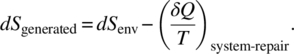
We note this heat can be related to energy cost to manufacture the repaired part. We see that by the second law (Equation (1.4)) ![]() . Therefore, this means that
. Therefore, this means that
This is as suspected that the repair process generates equal or more disorganized energy to the environment than the amount of organized energy needed for the repair process. This is evident in the solder joint example regarding the heat energy repair needed to reflow the solder joint. Sometimes the non-damage entropy flow to the environment is harmless; at other times, it may be very harmful and cause serious pollution issues.
Lastly, we would like to note that Mother Nature is a special case in which spontaneous entropy repair does exist. We have included this in the Special Topic Chapter C called “Negative Entropy and the Perfect Human Engine.”
We have now defined many useful terms, concepts, and key equations for system degradation analysis. The following chapter will provide many examples in equilibrium thermodynamics.
References
- [1] Feinberg, A. and Widom, A. (2000) On thermodynamic reliability engineering. IEEE Transaction on Reliability, 49 (2), 136.
- [2] Feinberg, A. and Widom, A. (1995) Aspects of the thermodynamic aging process in reliability physics. Institute of Environmental Sciences Proceedings, 41, 49.
- [3] Feinberg, A., Crow, D. (eds) Design for Reliability, M/A-COM 2000, CRC Press, Boca Raton, 2001.
- [4] Feinberg, A. (2015) Thermodynamic damage within physics of degradation, in The Physics of Degradation in Engineered Materials and Devices (ed J. Swingler), Momentum Press, New York.
- [5] Reynolds, W.C. and Perkins, H.C. (1977) Engineering Thermodynamics, McGraw-Hill, New York.
- [6] Cengel, Y.A. and Boles, M.A. (2008) Thermodynamics: An Engineering Approach, McGraw-Hill, Boston.
- [7] Khonsari, M.M. and Amiri, M. (2013) Introduction to Thermodynamics of Mechanical Fatigue, CRC Press, Boca Raton.
- [8] Bryant, M. (2015) Thermodynamics of ageing and degradation in engineering devices and machines, in The Physics of Degradation in Engineered Materials and Devices (ed J. Swingler), Momentum Press, New York.
- [9] Feinberg, A. and Widom, A. (1996) Connecting parametric aging to catastrophic failure through thermodynamics. IEEE Transactions on Reliability, 45 (1), 28.