
6
Thermal Activation Free Energy Approach
6.1 Free Energy Roller Coaster
Thermally activated processes are one of the four main types of aging described in Chapter 1. We now ask: how does the free energy change as degradation work occurs? Sometimes, the system path to the free energy minimum is smooth and downhill all the way to the bottom. For other systems, the path may descend to a relative minimum, but not an absolute minimum, something resembling a roller coaster. The path goes downhill to what looks like the bottom and faces a small uphill region. If that small hill could be scaled, then the final drop to the true minimum would be just over the top of the small hill. The small climb before the final descent to the true minimum is called a free energy barrier. The system may stay for a long period of time in the relative minimum before the final decay to true equilibrium.
Often the time spent in the neighborhood of the relative minimum is the lifetime of a fabricated product, and the final descent to the true free energy minimum represents the catastrophic failure of the product.
The estimated lifetime τ over which the system stays at the relative minimum obeys the Arrhenius law in Equation 5.21 as ![]() where Δφ is the height of the free energy barrier (φc).
where Δφ is the height of the free energy barrier (φc).
The activation energy can be thought of as the amount of energy needed for the degradation process. This defines a special relative equilibrium aging state
(6.1)
where the subscript B refers to the barrier and Δφ is the barrier height.
6.2 Thermally Activated Time-Dependent (TAT) Degradation Model
When activation is the rate-controlling process, Arrhenius-type rate kinetics applies. In this section, the parametric time-dependence of an Arrhenius mechanism is addressed. Parametric degradation is often termed “soft failure” or “device drift over time,” for example slow power loss of a transistor or creep change. This thermal activation mechanism explains logarithmic-in-time aging of many key device parameters described here. Such a mechanism, with temperature as the fundamental thermodynamic stress factor, leads to this predictable logarithmic-in-time-dependent aging on measurable parameters. Here the thermodynamic work is evident in the free energy path.
There are two thermally activated time-dependent (TAT) device degradation models [1, 2]. If degradation is graceful over time, then many instances occur in which logarithmic-in-time aging results for one or more device parameters. This aging and examples are described below. Degradation leading to catastrophic failure using the TAT model is presented at the end of this chapter, while applications for the TAT model are provided in the next chapter.
In Arrhenius processes, the probability rate dp/dt to surmount the relative minimum free energy barrier φ as in Figure 6.1 can be written
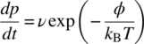
where ν is a rate constant; kB is Boltzmann’s constant; T is the temperature; and t is time. More information on this probability distribution is given in Section 6.3. We wish to associate the thermodynamic aging kinetics in the material with measurable parametric changes. Therefore, we model the above as a fractional rate of parametric change given by

where a is the fractional change of the measurable parameter. We can let a be dimensionless, defined ![]() . For example, ΔP could be a parameter change that is of concern such as resistance change, current change, mechanical creep strain change, voltage transistor gain change, and so forth, such that a is then the fractional change.
. For example, ΔP could be a parameter change that is of concern such as resistance change, current change, mechanical creep strain change, voltage transistor gain change, and so forth, such that a is then the fractional change.
In the TAT model the aging process is closely related to the parametric change. The assumption is that the free energy itself will be associated with the parameter through the thermodynamic work.

Figure 6.1 Arrhenius activation free energy path having a relative minimum as a function of generalized parameter a.
Source: Feinberg and Widom [1]. Reproduced with permissions of IEEE
Thus, φ will be a function of a as indicated in Equation (6.3). Then the free energy can be expanded in terms of its parametric dependence using a Maclaurin series (with environmental factor held constant for the moment). The free energy is defined:
where y1 and y2 are given by
6.2.1 Arrhenius Aging Due to Small Parametric Change
When a << 1, the first and second terms in the Maclaurin series yield

where  .
.
Rearranging terms, and solving for a as a function of t and integrating, provides a logarithmic-in-time aging TAT model where
where A and B are defined
Logarithmic-in-time aging is an important process since the origin of this aging kinetics can mathematically be tied to the Arrhenius mechanisms of which numerous examples exist [1, 2]. Figure 6.2 illustrates typical logarithmic-in-time aging. One notes that aging is highly non-linear for early time. This curve is representative of many aging and kinetic processes such as crystal frequency aging drift [3], corrosion of thin films, chemisorption processes [4], early degradation of primary battery life [5], activated creep (see Section 7.3), activated wear (see Section 7.2), transistor key parameter aging (see Section 7.4), and so forth. The significance of parametric logarithmic-in-time aging can further be put in perspective as it can be tied to catastrophic lognormal failure rates. As to why there is a connection in particular to the catastrophic lognormal failure rate distribution is explained in detail in Section 9.2 [1, 2].

Figure 6.2 Examples of ln(1 + B time) aging law, with upper graph similar to primary and secondary creep stages and the lower graph similar to primary battery voltage loss
Logarithmic-in-time aging has a similar form to a power law when the exponent of the time is between 0 and 1. For example
and
can both model the same physical degradation process. As an example, consider when A = 1.45, k = 0.5 in Equation (6.9) and when B = 2.2, a = 0.7 in Equation (6.10). Results in Figure 6.3 show how these two equations overlap graphically in modeling appearance.

Figure 6.3 Log time compared to power law aging models
The point is that many degradation processes in the literature, such as secondary creep, use empirical power-law models instead of the logarithmic model. However, a logarithmic-in-time model may equally be suitable for which a TAT model could be found. In this case, we might have a better understanding of the degradation process when physics can be applied to the degradation process to help understand what is occurring. Applications for the TAT model are provided in the next chapter.
6.3 Free Energy Use in Parametric Degradation and the Partition Function
Here we wish to describe more information on the probability distribution used in Equation (6.2). In statistical mechanics the Boltzmann distribution gives the probability that a system will be in a certain state as a function of the state’s energy and the temperature of the system.
In 1868 Ludwig Boltzmann formulated what is now a popular distribution for describing the probability for a system to be in a particular energy state as a function of the state’s temperature. The distribution is given by

where the system has a probability pi of being in the ith state; kB is the Boltzmann constant; T is the temperature of the system; N is the number of possible states that the system can be in; and the denominator Z is known as the partition function.
Just as the entropy has a statistical definition, the Helmholtz free energy is also related to the partition function
or we can write, from Equations (6.11) and (6.12), that the partition function is

The sum, often referred to as an ensample, can have a number of different internal energy states as shown in Figure 6.4a. The partition function near a true equilibrium state will have the free energy at a minimum; when the free energy is at a minimum, the value and the partition function will be at a maximum value. However, complex systems can have numerous degradation mechanisms each with their own relative minimum free energy equilibrium state, with relative maximum value for the partition function which for the ensemble of states are really the only contributing state in the sum that contribute to the value of Z as shown in Figure 6.4b. Therefore, the probability for a state to be occupied near an equilibrium state according to the ith relative minimum (where in Figure 6.4 i = 1, 2, or 3) is


Figure 6.4 (a) Continuous function with numerous energy states. (b) Relative minimum energy states having different degradation mechanisms
The activation energy of the ith failure mechanism, Ea,i, is related to the relative minimum barrier height (see Figure 6.1) which, using the partition function method and Figure 6.4b and according to Equation (6.12) is
The probability of a defect occurring then requires enough energy to surmount the free energy barrier created by the relative minimum in the free energy for the particular thermally activated failure mechanism, and is given by Equation (6.2):

We now can identify φ = F as the Helmholtz free energy, described in more detail by the activation energy through the Boltzmann distribution statistical mechanics. This identifies Equation (6.2) as useful in terms of a system’s free energy near either a relative minimum or a true equilibrium thermodynamic state. Note that the free energy can also be written in terms of the Gibbs free energy (see Equation (5.42), for example).
Now if the degradation of a system is a thermally activated mechanism, it is likely to have a relative minimum in the free energy. This can occur whether one is concerned with soft degradation over time having a parametric failure mechanism or even a catastrophic failure mechanism. Table 6.1 lists a number of different failure mechanisms with their typical known historical activation energies which have been observed. The method for measuring the activation free energy barrier height is exemplified in the Special Topics B section of this book. Systems are typically at a relative minimum for most of the lifetime of the product and do not catastrophically fail until enough defects have accumulated by gaining enough energy to jump over the free energy barrier. As defects accumulate at some point, the system loses its strength and catastrophically fails. This is the point where the system’s free energy has descended to its true minimum value which is its final equilibrium state, and the point where catastrophic failure occurs.
Table 6.1 Failure mechanisms and associated thermal activation energies
| Failure mechanism | Stress | Activation energy (eV) |
| Dielectric breakdown | Electric field, temperature | 0.2–1.0 |
| Corrosion | Temperature, humidity, voltage | 0.3–1.1 |
| Electromigration | Temperature, current density | 0.5–1.2 |
| Au–Al intermetallic growth | Temperature | 1.0–1.05 |
| Hot carrier injection | Electric field, temperature | 0.9–1.1 |
| Slow charge trapping | Electric field, temperature | 1.0–1.3 |
| Mobile ionic contamination | Temperature | 1.0–1.05 |
6.4 Parametric Aging at End of Life Due to the Arrhenius Mechanism: Large Parametric Change
In Section 6.2.1 we found aging due to small parametric change. Here we consider the second case for larger parametric change. A second TAT model can be obtained for both the initial aging period and end of life using both terms in the Maclaurin expansion in Equations (6.3) and (6.4) and performing the integration. The results obtained [1, 2] can be written:

where erf and erf−1 are the error function and its inverse, respectively, and
This model is a parametric aging phenomenon that ages similar to logarithmic-in-time models and quickly goes catastrophic at the end of its life due to Arrhenius degradation. This is illustrated in Figure 6.5. The figure shows that aging starts off similar to logarithmic-in-time aging, but then quickly goes catastrophic at the critical corresponding time tc [1, 2].

Figure 6.5 Aging with critical values tc prior to catastrophic failure.
Source: Feinberg and Widom [1]. Reproduced with permissions of IEEE
Figure 6.5 illustrates a number of rate processes that start off with log(time) aging then suddenly go catastrophic. Some examples exhibiting forms of this dependence over time are batteries [1], the three phases of creep, and cold-worked metals recrystallizing. What is interesting in this model is that the rate of initial aging is mathematically connected to its rate of final catastrophic behavior in this model. This suggests that, if the initial aging process is truly understood, a catastrophic prognostic may be possible.
References
- [1] Feinberg, A. and Widom, A. (2000) On thermodynamic reliability engineering. IEEE Transaction on Reliability, 49 (2), 136.
- [2] Feinberg, A. and Widom, A. (1996) Connecting parametric aging to catastrophic failure through thermodynamics. IEEE Transaction on Reliability, 45 (1), 28.
- [3] Warner, A.W., Fraser, D.B. and Stockbridge, C.D. (1965) Fundamental studies of aging in quartz resonators. IEEE Transaction on Sonics and Ultrasonics, 12, 52.
- [4] Ho, Y.-S. (2006) Review of second-order models for adsorption systems. Journal of Hazardous Materials, B136, 681–689.
- [5] Linden, D. (ed) (1980) Handbook of Batteries and Fuel Cells, McGraw-Hill, New York.