
4
Applications of NE Thermodynamic Degradation Science to Mechanical Systems: Accelerated Test and CAST Equations, Miner’s Rule, and FDS
4.1 Thermodynamic Work Approach to Physics of Failure Problems
We are now in a position to assess a number of reliability degradation problems. In this chapter we will continue to use the thermodynamic work to assess the entropy damage to the system and the amount of free energy left for numerous key problems in reliability. As we found in Chapter 3, the thermodynamic work is perhaps the most directly measurable and practical quantity to use in assessing a system’s free energy and its degradation [1–3]. This chapter provides many examples for deriving physics of failure aging laws and their acceleration factors in mechanical systems using the thermodynamic work principle.
4.2 Example 4.1: Miner’s Rule
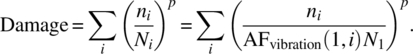
We derived the Miner’s rule using an entropy approach in Section 2.1.1. Here we derive it using the thermodynamic work approach [1–3]. Equation (3.25) for cyclic damage may be used to derive Miner’s empirical rule [4], commonly used for accumulated fatigue damage and a number of other useful expressions in damage assessment of devices and machines.
Consider a system undergoing fatigue as in the paper clip example, where we bend it back and forth a certain distance for three cycles. To find the actual work we need to sum the cyclic work area of each bend cycle since both the stress σ and strain e will change slightly as the paper clip fatigues. If we use Stokes theorem, it demonstrates the work is related to the cyclic area of each:

In Miner’s rule an approximation is actually made. Miner empirically figured that stress σ and cycles n were the main factors of damage.
In our framework this means
Miner also empirically assumed that the work for n cycles of the same cyclic size is all that is needed. In our framework this means
(Miner’s assumption versus reality, as work is reduced each σ cycles.)
Using this assumption, then we average the three cyclic areas of the same stress multiplied by three in our case:
Following this approximation, for any stress level we just count the number of cycles so that the total thermodynamic work is

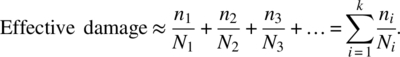
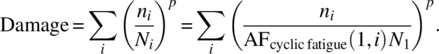
Using this approximation, we obtain effective damage (i.e., not the true damage) where the cumulative effective damage is:

or

Using the approximation above, the total work to failure is the same for each cyclic size type along the same work path so that
So this yields

giving

Therefore, Miner’s rule is an approximation of the cumulative fatigue damage, commonly written
An example of how to use Miner’s rule is given in Section 2.1.2. This is in agreement with what we found in Section 2.1.1 using the entropy approach. Equation (4.4) (also see Equation (3.25)) is a better estimate of the damage, as Equation (4.9) is based on the assumption that the stress is independent of the number of cycles tested. In fact we know from experience that, as the paper clip fatigues, it takes less stress to create the same bend amplitude.
4.2.1 Acceleration Factor Modification of Miner’s Damage Rule
It can be difficult to always know the cycles to failure at any ith stress level in Miner’s application. However, since we are on the same work path, we can often establish a cyclic acceleration factor (see Special Topic B for examples) between stress levels. If AFdamage and N1 are known, then Miner’s rule can be simplified from Equation (4.9) for the ith stress using
Then Miner’s rule can be modified as [3, 4]:

The acceleration factor AFdamage is given in Section 4.3.4 and depends on the type of vibration (sine or random). See also Section 4.5 for use of this equation in fatigue damage spectrum (FDS) analysis. It can also be used in thermal cycling (see Section 4.3.3).
4.3 Assessing Thermodynamic Damage in Mechanical Systems
In this section we will provide examples of how to apply the concept of damage to a number of mechanical systems of creep and wear, as well as an analysis for cyclic vibration and thermal fatigue.
4.3.1 Example 4.2: Creep Cumulative Damage and Acceleration Factors
Creep parameters include the strain (ε) length change ΔL (ΔL/L) due to an applied stress (σ) at temperature (T). In the elastic region, stress causes a strain that is recoverable (i.e., reversible) so that ![]() where Y is Young’s modulus. When stress increases such that the work is irreversible, the permanent plastic strain εp damage is termed plastic deformation. The most popular empirical creep rate equation is [3, 5]
where Y is Young’s modulus. When stress increases such that the work is irreversible, the permanent plastic strain εp damage is termed plastic deformation. The most popular empirical creep rate equation is [3, 5]
where B0 is a material strength constant; p is the time exponent where 0 < p < 1 for primary and secondary creep stages; M (where 0 < 1/M < 1) is strain hardening exponent, dependent on the material type; and Ea is the thermal activation energy for the creep process (see Figure 9.5 for the three stages of creep). We note a linear time dependence is observed in the secondary creep phase where p = 1. Some tabulated values are given in Table 4.1 for M and B0 for the secondary creep rate.
Table 4.1 Typical constants for stress–time creep law
| Material | Temperature (°C) | B0 (in2/lb)N per day | M |
| 1030 Steel | 400 | 48 × 10–38 | 6.9 |
| 1040 Steel | 400 | 16 × 10−46 | 8.6 |
| 2Ni-0.8Cr-0.4Mo Steel | 454 | 10 × 10−20 | 3.0 |
| 12Cr Steel | 454 | 10 × 10−27 | 4.4 |
| 12Cr-3W-0.4Mn Steel | 550 | 15 × 10−16 | 1.9 |
The thermodynamic work causing damage from the creep process of the metal is found from the stress–strain creep area when the stress–strain relation is plotted in Figure 4.1 to demonstrate typical creep data.

Figure 4.1 Creep strain over time for different stresses where σ4 > σ3 > σ2 > σ1
The conjugate work variables for creep are stress σ for force and ε = ΔL/L strain, the length variable. From Figure 4.1 displaying creep, we can see that it is logical to model the strain over time by a power law; the strain will also be a power law as a function of stress. We know from Equation (4.12) that these are good assumptions (see Figure 4.1), so that our general expression is
Furthermore, from Figure 4.1 it is logical that 0 < M < 1 for primary–secondary creep region (Figure 4.2).

Figure 4.2 Example of creep of a wire due to a stress weight
The thermodynamic work causing damage from the creep process depicted in Figure 4.2 is found from the stress–strain creep area when the stress–strain relation is plotted. Assessing the damage is more accurately found if the data were available. Here, we can use the empirical creep rate expression to find this area by integrating the expression above to determine the work in terms of the applied stress, which is more easily known. The creep path is dL (ε = ΔL/L) for the integral limits, so summing the thermodynamic work we have
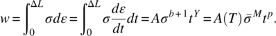
Making comparisons to the original empirical creep equation (Equation (4.12)), we have A(T) is defined within a constant ![]() , while
, while ![]() and Y = p. We have assumed that stress is not time dependent. Note that we prefer to use the term dε/dt for a constant stress to integrate over time to obtain damage in terms of the applied stress.
and Y = p. We have assumed that stress is not time dependent. Note that we prefer to use the term dε/dt for a constant stress to integrate over time to obtain damage in terms of the applied stress.
In order to assess the damage, we need to have some knowledge of the critical damage at a particular stress and temperature. Let’s assume this occurs at time τ1 at stress level σ1 and temperature T1. Then the thermodynamic damage ratio at any other stress σ2 and temperature T2 at time t2 along the same work path is

where ![]() and
and ![]() . Here, τi is time to failure (a constant) at stress i and ti is work time at stress level i. Again, this is valid for stresses 1, 2 along the same work path ΔL. If damage is 1, failure occurs (at t2 = τ2) and we can then write this as
. Here, τi is time to failure (a constant) at stress i and ti is work time at stress level i. Again, this is valid for stresses 1, 2 along the same work path ΔL. If damage is 1, failure occurs (at t2 = τ2) and we can then write this as

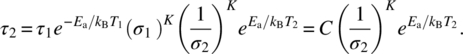
This is the creep acceleration factor (see Special Topic B on Acceleration Factor usage). Recall that ![]() (i.e., work to failure stress 2 and 1; see Equation (4.6)), so their ratio will be 1. Here M/p = K and Q = Ea/p. Often it is helpful to write the linear form for time to failure for a particular stress. This is deduced as follows from the above equation
(i.e., work to failure stress 2 and 1; see Equation (4.6)), so their ratio will be 1. Here M/p = K and Q = Ea/p. Often it is helpful to write the linear form for time to failure for a particular stress. This is deduced as follows from the above equation
Writing the time to failure tfailure for τ2 we have
where the constant C can always be written in terms of another stress if we know that ![]() ; however, it also equates to the factored-out constant in Equation (4.15) C = ln(1/A).
; however, it also equates to the factored-out constant in Equation (4.15) C = ln(1/A).
Lastly, it should be noted that if a number of different i stresses are applied, the general creep damage ratio can be written by accumulating the thermodynamic damage along the same work path (Equation (4.15)) as

In Section 4.5 and Special Topics B.7 we illustrate how this equation can be used for environmental profiling in order to find a cumulative accelerated stress test (CAST) goal.
4.3.2 Example 4.3: Wear Cumulative Damage and Acceleration Factors
Wear nicely exemplifies the thermodynamic approach. There are many different types of wear, including abrasive, adhesive, fretting, and fatigue wear. The most common wear model used for adhesive and sometimes abrasive wear of the softer material between two sliding surfaces is the Archard’s wear equation [6, 7]:
where D is removed depth of the softer material; PW is normal load (lb); l is the sliding distance (feet); H is hardness of the softer material (psi); A is contact area; and k is Archard’s wear coefficient (dimensionless). In the adhesive wear of metals [6–8], wear coefficient k varies between 10−7 and 10−2 depending on the operating conditions and material properties. It should be recognized that a wear coefficient k is constant typically only within a certain adhesive wear-rate range.
We define this as our system as shown in Figure 4.3, consisting of the weight, contact area, hardness, and k value and which is traveling at some velocity. Next we need to provide the environment which is responsible for doing work on our system which causes the movement so that wear can occur. We introduce an external force PE as shown in Figure 4.3.

Figure 4.3 Wear occurring to a sliding block having weight PW
PF creates the sliding and induces the thermodynamic wear work. Some of the external work goes into creating the wear velocity while some causes wear. Work is simply the integral of the force times distance or ![]() and dx is the sliding distance. It is logical that PF is proportional to PW, but since we are causing wear we write it as
and dx is the sliding distance. It is logical that PF is proportional to PW, but since we are causing wear we write it as ![]() . The distance dx can be written as
. The distance dx can be written as ![]() , where C2 is a constant related to the surface wear friction
, where C2 is a constant related to the surface wear friction

Note that the integral is over x1 to x2, the work path in the time t1 to t2, which is linear with wear amount. Since we have substituted vt for the sliding distance, we need to keep this in mind. Here we have introduced the knowledge of Archard’s wear model by identifying that our constant C2 is k/AH times some constant ![]() that is related to the work type. This constant is needed as without it we would just have Archard’s equation which has units of distance not work.
that is related to the work type. This constant is needed as without it we would just have Archard’s equation which has units of distance not work.
At some time t = τ1 we may consider that too much damage has occurred in a stress environment we call 1 as compared to stress environment 2. Then we can assess the damage ratio between environments 1 and 2, where 1 has caused failure and in 2 failure has not yet occurred:

where τ1 is the time for critical wear failure in stress environment 1. Note that for the two environments (1 and 2) the materials are the same so H and k cancel out. We must also stay on the same work type to make comparisons between environments; therefore kP are the same.
When failure occurs (the amount of wear is the same for both environments), the thermodynamic work in environment 2 equals that of environment 1, the damage ratio is 1, and ![]() . This occurs at time τ2 in environment 2, so we can then write the wear acceleration factor as
. This occurs at time τ2 in environment 2, so we can then write the wear acceleration factor as

(See Special Topics B for how to apply acceleration factors in testing.) The subscript DF indicates that we have created the same wear amount causing failure in both environments. One thing we note is that Archard’s type of wear is not easily accelerated as it is linear with weight and velocity.
It is helpful to write the linear form for time to failure for a particular stress. This is deduced to within a constant from the above equation

Then the time to failure for wear can be written tfailure = τ:
where C is a constant that can be written in terms of another stress level if known. However, it also represents the ratio of the factored-out constant ![]() .
.
If a number of different i stresses are applied along the same work path (Equation (4.22)). The general wear damage ratio can be written by accumulating the thermodynamic damage at each stress level as

In Section 4.3 and Special Topic B.7 we illustrate how this equation can be used for environmental profiling in order to find a CAST goal.
If the external force causes oscillator motion so that we are doing cyclic work for n cycles, we can replace t by n and τ by N to obtain Miner’s Rule for Archard’s type wear.
4.3.3 Example 4.4: Thermal Cycle Fatigue and Acceleration Factors
In thermal cycling, a temperature change ΔT in the environment from one extreme to another causes expansion and/or contraction (i.e., strain) in a material system. The plastic strain (ε) caused by the thermal cyclic stress (σ) in the material can be written similar to Equation (4.12) as:
where we have substituted σM ~ ΔT b for the non-linear stress and n for thermal cycles instead of time.
The thermodynamic work causing damage from thermal cycle stress is found from the stress–strain creep area if the stress–strain relation could be plotted. Then, similar to creep work above, the cyclic work is still over the path ΔL to Equation (4.14). However, the work path is not much of an issue in say solder joint expansion contraction or other joints that may have different expansion–contraction rates. The main concern is keeping the system, such as the solder joint, consistent during analysis. We have

where ![]() . We need to have some knowledge of the critical damage at a particular cyclic stress and along this work path. Let’s assume this occurs at N1 at stress level ΔT1. Then, similar to Equation (4.15), the damage ratio at another stress ΔT2 for n2 cycles is
. We need to have some knowledge of the critical damage at a particular cyclic stress and along this work path. Let’s assume this occurs at N1 at stress level ΔT1. Then, similar to Equation (4.15), the damage ratio at another stress ΔT2 for n2 cycles is

If damage is 1 then ![]() , failure occurs and we write the acceleration factor
, failure occurs and we write the acceleration factor

where ![]() and
and ![]() . The non-Arrhenius ratio is called the “Coffin-Manson” acceleration factors [9–11], or Equation (4.30) is the Modified Coffin-Manson acceleration factor. When the activation energy Ea is small then the Arrhenius effect can be neglected. For example, in solder joint testing, K = 1.9 for lead-free solder and about 2.5 for lead solder. The activation energy is about 0.123 eV that is typically used. For example, if use condition is stress level 1 cycle between 20 and 60 (ΔT = 40°C, Tmax = 60°C), while test stress condition is stress level 2 cycled between −20 and 100°C (ΔT = 120°C, Tmax = 100°C), then Arrhenius AF = 1.58 while the Coffin-Manson AF = 9 with an overall AF of 14.2. In the case where we have 1 cycle per day in use condition, we see that 10 years of use condition is about 260 test cycles (see Special Topics B for more applications).
. The non-Arrhenius ratio is called the “Coffin-Manson” acceleration factors [9–11], or Equation (4.30) is the Modified Coffin-Manson acceleration factor. When the activation energy Ea is small then the Arrhenius effect can be neglected. For example, in solder joint testing, K = 1.9 for lead-free solder and about 2.5 for lead solder. The activation energy is about 0.123 eV that is typically used. For example, if use condition is stress level 1 cycle between 20 and 60 (ΔT = 40°C, Tmax = 60°C), while test stress condition is stress level 2 cycled between −20 and 100°C (ΔT = 120°C, Tmax = 100°C), then Arrhenius AF = 1.58 while the Coffin-Manson AF = 9 with an overall AF of 14.2. In the case where we have 1 cycle per day in use condition, we see that 10 years of use condition is about 260 test cycles (see Special Topics B for more applications).
Equation (4.30) is also similar to the Norris–Lanzberg [12] thermal cycle model which also includes a thermal cycle frequency effect (see Equation (B18) for details and uses of their model).
It is helpful to write the linear form for cycles to failure for a particular stress. This is deduced as

The thermal cycles to failure is therefore
where C can be written in terms of the other stress factor if known, ![]() . However, it can also be found as the factored-out ratio constant C = ln(1/B).
. However, it can also be found as the factored-out ratio constant C = ln(1/B).
Lastly, it should be noted that if a number of different stresses are applied the general damage ratio can be written by accumulating the thermodynamic damage along the same work path (Equation (4.29)) as in Miner’s rule:
In Section 4.4 and Special Topics B.7 we illustrate how this equation can be used for environmental profiling in order to find a CAST goal.
4.3.4 Example 4.5: Mechanical Cycle Vibration Fatigue and Acceleration Factors
In a similar manner to the above argument for thermal cycle, we can find the equivalent mechanical vibration cyclic fatigue damage. In a vibration environment, a vibration level depends on the type of exposure. In testing two types of environments are typically used: sinusoidal and random vibration profiles. In sinusoidal vibration the stress level is denoted Gs, where G is a unitless quantity equal to the sinusoidal acceleration A divided by the gravitational constant g. In random vibration, a similar quantity is used termed Grms (defined below). Consider first the plastic strain (ε) caused by a sinusoidal vibration level G stress (σ) in the material. The strain can be written similarly to Equation (4.27):
The cyclic work is then found, similar to Equation (4.28), as

where Y = j + 1. Similar to the above arguments, to assess the damage we need to have some knowledge of the critical damage at a vibration stress. Let’s assume this occurs at N1 at stress level G1. Then, as in Equation (4.29), the thermodynamic damage ratio at any other stress G2 level at n2 cycle is

If damage is 1, n2 = N2, and failure occurs. Following the arguments of the other examples, we find the acceleration factor is

where b = Y/P. Since the number of cycles is related to cycle frequency f and the time τ according to
then if f is constant AFdamage is a commonly used relationship for cyclic compression where

This is commonly used for the acceleration factor in sinusoidal testing. For random vibration above, we substitute for G the random vibration Grms level [13] (see Special Topics B for examples).
It is helpful to write the linear form for cycles to failure for a particular stress. This is deduced to within a constant from the above equation
where ![]() is treated as a constant. This is essentially the relation that holds for what is called the S–N curves (see Figure 1.3). Note that if we write the cyclic equation with G ∝ S where S is the stress, we have
is treated as a constant. This is essentially the relation that holds for what is called the S–N curves (see Figure 1.3). Note that if we write the cyclic equation with G ∝ S where S is the stress, we have
where ![]() , C is the proportionality constant when going from G to S, and K is a constant similar to C. Note that some authors write this as proportional to the strain instead of the stress. The relationship is generally used to analyze S–N data. b and C are often referred to as Basquin’s equation, commonly written as
, C is the proportionality constant when going from G to S, and K is a constant similar to C. Note that some authors write this as proportional to the strain instead of the stress. The relationship is generally used to analyze S–N data. b and C are often referred to as Basquin’s equation, commonly written as
Note that since stress and strain are conjugate variables, one can write this alternately in terms of the strain. However, it is usually written this way as the experimental number of cycles to failure N for a given stress S level constitutes S–N curve data in fatigue testing of materials. Such data are widely available in the literature. The slope of the S–N curve (see Figure 1.3) provides an estimate of the exponent b above. S–N data are commonly determined using sinusoidal stress. Often we do not know b. Typical values of b are 4 < b < 8. Some guidance is provided in MIL-STD-810F. For example, it recommends b = 8 for broadband random (discussed below) and b = 6 where for profiles. A conservative test is obtained by setting b = 4. Testing can of course can determine b for a particular failure mode.
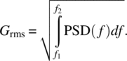
Most device vibration testing is typically either sinusoidal or random. The goal is to try and accelerate the type of vibration occurring under use conditions. For automotive, for example, this is random vibration. For a piece of equipment undergoing cyclic motion, this is more likely sinusoidal. The relation for random data is b/2 when using the power spectral density (PSD) (Grms2/Hz) level instead of Grms. This is evident from the fact that the Grms level is found as the square root of the area under the PSD spectrum:
In the simple case of random vibration, white noise for example, we have
Here the time compression expression above for random vibration is over the same bandwidth ![]() , then inserting Equation (4.44) into Equation (4.39) we have
, then inserting Equation (4.44) into Equation (4.39) we have

This is a common form used for the random vibration acceleration factor [13] (see Special Topics B for examples). The general form for the cycles to failure for a particular stress is then
Finally, it should be noted that if we have applied a number of different stresses, the general damage ratio can be written by accumulating the thermodynamic damage along the same work path (Equation (4.36)) as
This equation turns out to be extremely useful. In Section 4.4 and Special Topics B.7 we illustrate how this equation can be used for environmental profiling in order to find a CAST goal.
4.3.5 Example 4.6: Cycles to Failure under a Resonance Condition: Q Effect
When a product has a built-in resonance that is causing a higher stress level, the fatigue life will be shortened due to magnification of the resonance. In order to model the resonance condition for fatigue life, we first need to explain some common resonance terms to aid the unfamiliar reader. Resonance is commonly quantified using an amplitude magnification factor denoted Q which is typically measured in a number of ways. Figure 4.4 illustrates a resonance. The most common way to measure a resonance is through the transmissibility. The transmissibility is the output divided by the input peak G or Grms level. This is illustrated for sinusoidal vibration in Figure 4.4, giving

Figure 4.4 Graphical example of a sine test resonance
An alternate way to measure Q when the resonance curve is available but the input level is not known is by assessing the resonance value f0 divided by the resonance width Δf at the maximum amplitude, divided by the square root of 2 as illustrated in Figure 4.4, and given by
Since we have already quantified the cycles to failure in terms of the G or Grms level, then under a resonance condition the output G level is simply multiplied by the Q magnification level at resonance so the time to failure is
Here Grms(Q) indicates that the Grms level is a function of Q. We see the cycles to failure generally goes as the input G-level multiplied by Q for sinusoidal vibration to an inverse power, so that larger Q and/or G values yield a smaller number of cycles to failure. Recall that since time is related to cycles through the frequency of vibration as time = N-cycles/frequency, then we can put this in terms of time to failure if needed.
If we have a random vibration input then the Grms level is not easily assessed. The simplest instructional way to estimate the Grms level from the input PSD level at resonance is to use the well-known Miles’ equation [14, 15], defined:

Miles’ equation is applicable for a single degree of freedom. It is an approximate formula that assumes a flat power spectral density in the neighborhood of the resonance f0. As a rule of thumb, it may be used if the power spectral density is flat over at least two octaves centered at the natural frequency. To ensure narrow band resonance over a flat portion of the spectrum, a Q ~ 10 or higher is often recommended.
As an example for using the Miles’ equation, if we have a single degree of vibration system with an 80 Hz resonance having a Q of 12 and a random 0.04 Grms2/Hz input level then the Grms resonance level at resonance is estimated as:

Random vibration is not simple to understand. As the term suggests, the input vibration levels are not constant but are random in nature. Therefore, there is a probability of occurrence in amplitude. The Miles’ equation above is written in terms of a 1-sigma response which means then when the random vibration is roughly Gaussian that this Grms level occurs about 68.27% of the time. Since Miles’ equation stipulates that the PSD be approximately flat near the resonance condition, then this is atypical for a Gaussian-like input in the frequency domain.
Using Miles’ equation, the time to failure can therefore be written for a single degree of freedom where the natural frequency response to a random vibration input can be approximated as above for a Q ∼ 10 or higher and a flat PSD input near f0 and, under these conditions, will occur about 67% of the time (1-sigma) as
It is important to note that Q is the inverse of damping as
where ξ is the damping factor and η is the loss factor. Often materials are characterized using the loss factor [3] and it is helpful to know which materials can be used to reduce resonances. Table 4.2 provides a list of typical well-known loss factors for different materials.
Table 4.2 Damping loss factor examples for certain materials
| Material | Damping loss factor (η) |
| Metals | <0.01 |
| Steel | 0.001–0.002 |
| Aluminum | 0.007–0.005 |
| Rubber (depends on type) | 0.01–0.05 |
| Frictional spring | 0.1–0.5 |
4.4 Cumulative Damage Accelerated Stress Test Goal: Environmental Profiling and Cumulative Accelerated Stress Test (CAST) Equations
A very important use of the cumulative stress equations in this chapter is in accelerated testing goals by doing proper environmental profiling of fielded stress conditions. These equations can help as they already define the cumulative stress damage equations. To that end, we would like to define a new term here called the CAST goal. The CAST goal depends on the work path, that is, the type of stress, and the total fielded use time τ1 (or N1 cycles) needed to design a test for 10 years or 20 000 cycles, for example. We may not know the time to failure N1 or t1, but we may only need 10 years of life or equivalent cycles. If we survive this equivalent damage time on an accelerated test, then we have proven that our product can survive the fielded use time it is designed for by doing a properly designed accelerated test using the CAST goal.
The issue is that a product in the field is typically exposed to varying stresses over time, so how do we specify one CAST goal and at what equivalent stress level? We do this by cumulating all the i stresses and associated times at each ith environmental stress relative to one particular reference stress of interest we call Stress 1. If this were say temperature with numerous estimated temperature profiles in the field, we collapse it to something like 10 years at 50°C. Obviously if there is only one constant temperature, for example 50°C, that a product is exposed to in the field, we do not need to cumulate the fielded environments and collapse them as we already know the fielded stress and simply define the time goal of say 10 years. Table 4.3 provides some very common CAST goals for different fielded stress work path types. Note that we have included Equation (5.10) from the next chapter for completeness. To illustrate how to use CAST goals, an example is provided in Section B7.1.
Table 4.3 Cumulative stress test goals: CAST equations
| Stress (work path) | Original equation | CAST equations and goal* (survival time or no. cycles) |
| Fatigue (Miner’s Rule) | (4.11) |  |
| Creep | (4.19) |  |
| Wear | (4.26) |  |
| Thermal cycle | (4.33) | 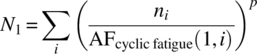 |
| Vibration | (4.33) |  |
| Temperature (corrosion) | (5.10) |  |
* AFdamage is the damage acceleration factor defining the work path.
4.5 Fatigue Damage Spectrum Analysis for Vibration Accelerated Testing
In vibration theory, the method for assessing damage has broadened to the use of spectral information. Often we would like to accelerate field data in vibration testing to simulate product life in the lab in a short time frame. However, field data spectrums are difficult to reproduce and accelerate correctly as, in reality, a product experiences lots of different types of vibration during its life. A great tool was developed to help reproduce potential field data damage to representative field spectra, called fatigue damage spectrum (FDS). Once FDS field data are obtained, a test engineer can statistically simulate the end-use environment to test their product. Once the end-use environment is simulated, the test engineer can accelerate a test to a desired test duration value more accurately. In addition, a test engineer can predict the life expectancy of a product by adjusting the target life to produce a desired spectral excitation for a test. Such FDS software is now available [16].
FDS is based on Miner’s Rule for damage where fatigue damage accumulates in a product until it fails. In FDS theory, using Miner’s rule the total damage a product experiences in a particular time can be calculated from field data and plotted for a specific range of frequencies. The resulting plot of fatigue damage versus frequency is the FDS, a means by which to quantify the stress–strain loads placed on a product.
Field data are collected by accelerometers that record the vibration levels at a number of positions on the product in the field under use condition of concern (i.e., likely worst-case fatigue conditions). The fatigue damage dosage for each maneuver is calculated using an FDS, which effectively plots damage versus frequency. The damage from each field use condition of concern is summed over the usage profile of the product to estimate the likely life accumulated damage. From this profile we determine a statistically representative vibration test which contains at least the same damage content as the product’s lifetime, but over a short test period.
FDS theory exists for both sine and random vibration testing. We start with sine vibration as it is typically easier to illustrate, then we explain it for random vibration.
The use of random vibration for testing is often used instead of sine vibration as it more often than not represents real-world situations. Random vibration is mostly analyzed by a spectrum in the frequency domain rather than the time domain. Random vibration is then as the name indicates: random. Its actual distribution depends on test requirements.
4.5.1 Fatigue Damage Spectrum for Sine Vibration Accelerated Testing
In sine vibration, we create cyclic fatigue. The input G level will cause a stress on the components and can cause cyclic fatigue that we described in Equation (3.23). The G stress level even in sine vibration will vary with frequency, and Equation (3.25) cyclic damage can be written

If we knew the cyclic work area at each test frequency point, perhaps with the use of a strain gage, we could accumulate the amount of work that was done in some period of time where cycles n = f × (test time). Often it is approximated using Miner’s rule, so we can write the damage over a resonance point due to frequency test from fmin < fn < fmax as:

where di is the damage at the ith stress level which varies with frequency. This of course is an alternate form of Miner’s Rule (Equation (4.9)). For example,

where we have used Equation (4.42) (N = CS−b) as in Equation (4.11). The stress level will go as the vibration amplitude, denoted here as Z(f) (function of frequency f) to within a K factor, S(f) = KZ(f), so we write the fatigue damage spectra as [17–20]

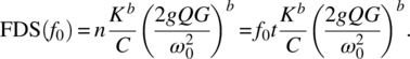
4.5.1.1 Example 4.7: Fatigue Damage Spectrum for Sine Vibration at and across Resonance
At resonance, we only have one stress level i so that n simply equates to ![]() (where t is the test time). Next in sine testing the displacement is defined
(where t is the test time). Next in sine testing the displacement is defined ![]() , where ω0 is the resonance frequency. The acceleration is the second derivative so the maximum acceleration = Zω02 and the acceleration in terms of Gs is gG, so that
, where ω0 is the resonance frequency. The acceleration is the second derivative so the maximum acceleration = Zω02 and the acceleration in terms of Gs is gG, so that ![]() . However, the peak to peak displacement is what is needed so this is a factor of 2 difference; furthermore, since we are at resonance we must take into account the amplification factor Q at resonance (see Figure 4.4) so
. However, the peak to peak displacement is what is needed so this is a factor of 2 difference; furthermore, since we are at resonance we must take into account the amplification factor Q at resonance (see Figure 4.4) so ![]() . Then Miner’s rule for fatigue testing at a sinusoidal resonance yields the following FDS spectrum:
. Then Miner’s rule for fatigue testing at a sinusoidal resonance yields the following FDS spectrum:
If we are testing across the resonance, then the amplitude is given by

The denominator is found from the harmonic oscillator amplitude equation which is found in numerous books and articles. It is not reproduced here as it is easily referenced.
4.5.2 Fatigue Damage Spectrum for Random Vibration Accelerated Testing
In a very similar manner we can use the concepts for random vibration. We will consider looking at the general damage spectrum (GDS) near a resonance (that will be related to FDS shortly) in random vibration. Then we will have, similar to Equation (4.58),
In random vibration FDS theory, the stress is proportional to the relative displacement of the single degree of freedom (SDOF) (i.e., single axis) multiplied by a constant K:
When the test vibration distribution is Gaussian, Mile’s equation is in many cases a good estimate for the Grms displacement that takes place. That is, there is a certain probability for displacement amplitudes. Using Mile’s equation (Equation (4.51)), this is:

By inserting Equations (4.63) and (4.62) into (4.61), we have for the general damage fatigue spectrum for any ith SDOF narrow-band random vibration Gaussian

Finally, the FDS differs from the GDS theory by what is called the expected values for the amplitude for a narrow-band Gaussian, which only differs by a gamma numeric factor that goes with b as shown below

These data in the field are collected over the ith WPSD-input narrow-band Gaussian areas of frequency, as these are worst cases. Then the FDS is generated for the environment. In general, the constants are taken as K = C = 1, the exponent b = 4, 8, or 12 (see discussion in Section 4.3.4) and the amplification factor Q = 10, 25, or 50. The inverse of this equation reproduces the test spectrum and is written

Once we have the test profile, W(f) the actual test-level W(f)-Test is specified by changing the t to teq for the test to accelerated time. This is consistent with Equation (4.46) when time is put in terms of cycles to failure. Typical values for b or G according to the Mil-Std 810F are around 8.
References
- [1] Feinberg, A. and Widom, A. (2000) On thermodynamic reliability engineering. IEEE Transaction on Reliability, 49 (2), 136.
- [2] Feinberg, A. Using Thermodynamic Work for Determining Degradation and Acceleration Factors. ASTR 2015 (available also at http://www.dfrsoft.com, accessed 5 May 2016).
- [3] Feinberg, A. (2015) Thermodynamic damage within physics of degradation, in The Physics of Degradation in Engineered Materials and Devices (ed J. Swingler), Momentum Press, New York.
- [4] Miner, M.A. (1945) Cumulative damage in fatigue. Journal of Applied Mechanics, 12, A159–A164.
- [5] Collins, J.A., Busby, H. and Staab, G. (2010) Mechanical Design of Machine Elements and Machines, 2nd edn, John Wiley & Sons, Inc., New York.
- [6] Archard, J.F. (1953) Contact and rubbing of flat surface. Journal of Applied Physics, 24 (8), 981–988.
- [7] Archard, J.F. and Hirst, W. (1956) The wear of metals under unlubricated conditions. Proceedings of the Royal Society, A-236, 397–410.
- [8] Hirst, W. (1957) Proceedings of the Conference on Lubrication and Wear, Institution of Mechanical Engineers, London, p. 674.
- [9] Coffin, L.F. (1954) A study of the effects of cyclic thermal stresses on a ductile metal. Transactions of the ASME, 76, 923–950.
- [10] Coffin, L.F. (1974) Fatigue at high temperature: prediction and interpretation. James Clayton Memorial Lecture. Proceedings of the Institution of Mechanical Engineers (London), 188, 109–127.
- [11] Manson, S.S. (1953) Behavior of Materials under Conditions of Thermal Stress, NACA-TN-2933 from NASA, Lewis Research Center, Cleveland.
- [12] Norris, K.C. and Landzberg, A.H. (1969) Reliability of controlled collapse interconnections. IBM Journal of Research and Development, 13 (3), 266–71.
- [13] MIL-STD-810G. 2008. Method 514.6, Military Standard 810G, Annex A, 31 October 2008.
- [14] Miles, J.W. (1954) On structural fatigue under random loading. Journal of the Aeronautical Sciences, 21, 753.
- [15] Steinberg, D.S. (2000) Vibration Analysis for Electronic Equipment, Wiley-Interscience, New York.
- [16] Vibration Research Corporation is one good source that provides FDS software and helps implement the process. See http://www.vibrationresearch.com, accessed on 4 May 2016.
- [17] Downing, S.D. and Socie, D.F. (1982) Simple rainflow counting algorithms. International Journal of Fatigue, 4, 31–40.
- [18] Bishop, N.W.M. and Sherratt, F. (1989) Fatigue life prediction from power spectral density data. Part 2: recent development. Environmental Engineering, 2 (1 and 2), 5–10.
- [19] Halfpenny, A., Kihm, F. Mission profile and testing synthesis based fatigue damage spectrum. Proceedings of the 9th International Fatigue Congress, 2006, Atlanta.
- [20] McNeill, S.I. Implementing the Fatigue Damage Spectrum and Fatigue Equivalent, Vibration Testing, Sound and Vibration. Proceedings of the 79th Shock and Vibration Symposium, October 26–30, 2008, Orlando, FL, pp. 1–20.