5.1 Corrosion Damage in Electrochemistry

We have noted that the Helmholtz free energy equated to work at constant temperature (T) and sometimes we also used constant volume (V) (see Equation (2.99)). Similarly, for constant temperature and pressure (P) corrosion processes, the change in the Gibbs free energy G bounds the ability to do useful work (see Section 2.11.3).

In detail, the change in the Gibbs free energy is given by

From the first law we have that the internal energy is the heat minus any type of work, which we describe as compressive and non-compressive:

Then substituting this equation into ΔG for quasistatic isothermal processes we can write as in Equation (2.108)

(5.1)

Therefore, the Gibbs free energy bounds the work process. In actuality, for many corrosion processes we will be able to determine the corrosion damage from the thermodynamic work done as they are reasonably quasistatic, so that

The equality for a reversible process in Equation (5.1) indicates that the free energy is the reversible work. As we found in Chapter 3, we can therefore interpret the above equation as a statement for the thermodynamic work in the form

In this section we provide some examples of how to use the concept of work damage in electrochemistry. We include examples for Miner’s rule for secondary batteries, chemical corrosion processes, corrosion current in primary batteries, and corrosion rate in microelectronics. In Chapter 1 we described four main types of aging. Corrosion is in the category of a complex aging process. It often involves thermal activation, forced electrical excitation, and can also include mechanical issues such as stress corrosion cracking. We can often separate these by looking at the rate-controlling mechanism. There are a number of ways to look at corrosion processes in electrochemistry. We start with an unusual treatment in the following example by applying a Miner’s rule application.

5.1.1 Example 5.1: Miner’s Rule for Secondary Batteries

Miner’s rule is not limited to mechanical stress; it can be applied to many types of cyclic fatigue situations.

For example, one interesting application is to chemical cells of secondary batteries [1, 2]. Here the cyclic work from Table 1.1 for k charge–discharge cycles is

(5.2)

In an analogous manner, battery manufacturers plot something similar to S–N curves found in mechanical stress–strain application. This is depth of discharge percent (DoD%) versus charging–discharging cycles to failure N. However, by comparison, in this case the DoD strain variable, charge is plotted using the DoD% (which is a percent of the charging capacity). This is plotted instead of the stress cycles to failure by battery manufacturers for an apparent stress failure threshold of voltage as shown in Figure 5.1.

In an application of Miner’s rule for secondary batteries using such available data the sum is over the DoD% ith level for battery life pertaining to a certain failure (permanent) voltage drop (such as 10%) of the initially rated battery voltage. Then the effective damage done in n_i DoD% can be assessed when N_i is known for the ith DoD level. For k-types of DoD% for various ith levels, Miner’s rule for secondary battery takes on the familiar form

(5.3)

where n and N are related to the number of DoD taken for the ith DoD level. The S–N type of DoD% curve is modeled [1, 2] as chemical rate where activation plays a role in battery N cycle life:

(5.4)

This is plotted in Figure 5.1. Here we assume the activation free energy is a linear function of depth of discharge [1, 2] (see Equation (5.26) and Chapter 6 for details of the activation free energy):

(5.5)

where ν is the activation damage voltage; Q_j is the value for which the battery manufacturer assumes the chemical cell to be fully discharged for the jth battery type (see Equation (5.2)); and φ is a damage activation energy. We then define

(5.6)

5.2 Example 5.2: Chemical Corrosion Processes

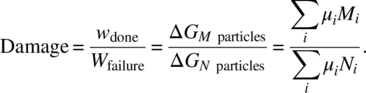
In a corrosion process we have from Table 1.1 that the Gibbs work is μ dN where we have N_i particles (or mole) of species i reacting. If the total reaction is consumed after N_i particles, and the reaction proceeds to the point where only M_i < N_i particles have reacted, then we can immediately determine the damage from the thermodynamic work. The resulting work done on the chemically reacting system may be described in terms of the chemical potential μ_i of the species k. That is, under constant temperature and pressure, the work is directly related to the Gibbs free energy change so the damage is defined, from Table 1.1 and Equation (2.114),

(5.7)

However, chemical potentials are not easily assessed. Further, this says very little about the rate of the reaction. The expression is therefore not easily quantified. We need to work with measurable parameters that are available. For example, we may know the corrosion rate or corrosion current under a certain stress condition. Then instead of using the chemical potential approach to assess damage, we can default to the thermodynamic work rule. For example, using the corrosion current (Table 1.1), the work is . A primary battery is an example where the V and I are known and the battery degradation is due to chemical cell corrosion. If V–I is not a rate-controlling stress and temperature is instead, we will show how to use this. Although we do not have cyclic work, we can think of it in terms of corrosion time for a single cycle. Then considering the corrosion time, we write the corrosion damage

(5.8)

where for the ith stress condition (e.g., temperature stress i), t_i is the corrosion time and τ_i time to fail. We find the expression simplifies and we do not actually need to know the corrosion current–voltage at any stress level if we know the time to failure τ_i at each ith stress level, similar to Miner’s rule. We can view this for general, galvanic, or specific corrosion processes such as primary batteries.

It can be difficult to always know the failure time at any ith stress level. However, since we are on the same work path, we can often establish an acceleration factor between stress levels. If AF_C (C for corrosion acceleration factor) and r₁ are known, then the above equation can be simplified for the ith stress using

The term AF_{corr damage} will be related to the corrosion rate which, in the most general form from above, will be between the ith and jth stress environment. Similar to how we found the acceleration factors in Chapter 4, using Equation (5.7) we find

(5.9)

Note that the corrosion current in general will also be a function of the ith stress temperature T_i. That is, temperature may need to be added to the acceleration factor (see Equation (5.20)). Below we develop a number of other expressions for AF_damage that may be of interest. Then the damage equation for corrosion can be simplified as

(5.10)

The equation turns out to be extremely useful. In Section 4.4 and Special Topics B.7 we illustrate how this equation can be used for environmental profiling in order to find a cumulative accelerated stress test (CAST) goal in the form of

(5.11)

When our product is subjected to multiple stresses in the field, we will find a certain amount of corrosion damage at τ₁ (say 5 years). If we wanted to design an accelerated test to simulate this damage, how do we select one equivalent stress? Equation (5.11) will allow us to profile and find one overall representative equivalent stress that would equate to this same amount of damage observed at τ₁. Once we have one equivalent stress for the damage amount at τ₁ we have an environmental profile and can design an accelerated test that will accelerate time and create the same damage amount in a shorter period of test time as observed in the field (at 5 years). An example is provided in Special Topics B.7.1.

Now consider the case when the damage value is 1; failure occurs and we can derive a useful expression for the acceleration factor in terms of the stress. However, in this case we will first need an expression for the corrosion rate.

A common expression for the corrosion rate in terms of mass transferred in the reaction [3] is given according to Faraday’s Law (dM/dt) as proportional to the net current I(T), a function of the reaction rate in temperature (discussed below) as

(5.12)

where dM is the mass of metal dissolving (g) and

(5.13)

Thus, A_m is the atomic mass. The corrosion rate (dM/dt) is then

(5.14)

5.2.1 Example 5.3: Numerical Example of Linear Corrosion

It can be confusing to use the equation. As a simple example, consider iron corroding in air-free acid at an electrochemical corrosion rate of 1 μA/cm². It dissolves as ferrous ions (Fe⁺²) and therefore n = 2. We can obtain the corrosion rate in mils per year (mpy) using the above expression

(5.15)

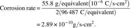
To convert the corrosion rate to mpy, first divide by the density of iron (7.86 g/cm³). Additionally there are 3.15 × 10⁷ s/year and 393.7 mils/cm (=1 inch/2.54 cm × 1000 mils/inch), then

(5.16)

Corrosion rate = 0.456 mpy.

Here mpy is a common corrosion rate unit. Table 5.1 provides relative values for estimating corrosion resistance of materials. From the table, note that 0.46 mpy is an outstanding corrosion rate, indicating an excellent corrosive resistive material. Note this table of relative values is established under a certain set of environmental conditions.

Relative corrosion resistance	Mils per year (mpy)	Micrometer per year (µm/year)
Outstanding	<1	<25
Excellent	1–5	25–100
Good	5–20	100–500
Fair	20–50	500–1000
Poor	50–200	1000–5000
Unacceptable	200+	5000+

When the corrosion rate is linear, the rate can be found by simply dividing the mass corroded by the corrosion time. In units of R (cm/h), this is the mass W with exposed area A in a laboratory experiment, defined

(5.17)

Here, the expression can be checked using its units. Now converting to a mixed unit expression, the conversion factor R(cm/h)(3.44 × 10⁶ mils/cm × h/year) gives R in mpy. Thus, R(cm/year) = 1/(3.44 × 10⁶) R(mpy). Since A(cm²)(inch²/(2.54 cm)²) gives A in inch², then A(cm²) = 6.45 A(inch²). Similarly, W(g)/1000 = W(mg). Inserting these values into the above equation, we have

(5.18)

This is one common mixed unit expression used in corrosion engineering.

5.2.2 Example 5.4: Corrosion Rate Comparison of Different Metals

Using Faraday’s law we can make a comparison of the corrosion amount and rate for different metals. Consider an experimental set-up as shown in Figure 5.2. Let the anode be various metals. The cathode can be say stainless steel (iron). Let us consider a corrosion current flowing of 5 mA for 1 year. Table 5.2 provides the calculated results using Faraday’s linear law of corrosion.

As an example of one of the calculations, the amount of metal removed for iron in 1 year at 5 mA is 45.6 g. This is found as

If we were trying to find an electrode with the least amount of corrosion mass, we note that titanium is the best choice. However, if cost was a consideration, stainless steel (iron) would likely be the second-best choice.

Metal	Atomic weight (g/mol)	Outer shell electrons	Density (g/cc)	Rate (mpy)	Corrosion amount (g)
Copper	63.55	1	8.96	4558	103.8
Iron	55.8	2	7.874	2277	45.6
Brass*	64.15	2	8.3561	2467	52.4
Titanium	47.88	2	4.54	3389	39.1
Nickel	58.69	2	8.9	2119	48.0
Tin	118.71	4	7.31	2609	48.5
Zinc	65.39	2	7.13	2947	53.4
Indium	114.8	3	7.31	3364	62.5
Lead	207.2	4	11.35	2933	84.7
Tungsten	183.85	2	19.25	3069	150.2
Iridium	192.22	2	22.4	2757	157.1
Silver	107.86	1	10.5	6602	176.3

* 67Cu.33Zn.

5.2.3 Thermal Arrhenius Activation and Peukert’s Law

The corrosion current is dependent on the actual situation, but in general is thermally activated across a free energy barrier

(5.19)

This is the well-known Arrhenius dependence which can be written either using R, the gas constant, given as 8.31 J/K mole and E_R is in joules, or using k_B, the Boltzmann constant (8.6173 × 10⁻⁵ eV/K) with E_a in electron-volts (eV). The gas constant is more commonly used in electrochemistry than the Boltzmann constant. I₀ is current rate constant for generalized corrosion current. We can now consider two different environments at different temperatures. If we have obtained a damage value of 1 between these two stress environments, then from Equations (5.8) and (5.19):

(5.20)

Here we have let V₁ = V₂ since temperature often dominates the corrosion process. This is the well-known Arrhenius acceleration factor (see Special Topics B for application of this factor). The rate for any one stress is

(5.21)

where ν is a rate constant (which could be written in terms of another rate using the acceleration factor in Equation (5.20) if known, e.g., ). We note that E_a is often thought of as a barrier height. The barrier height is a property of the system’s free energy related to the type of material (see Chapter 6 for more details). The expression is often written in linear Y = ax + b form so that the time to failure can be plotted for regression analysis as

(5.22)

where C is simply ln(1/ν).

Note that the voltage potential usually does not factor in different stress temperatures; only the current (often a function of voltage) will likely change or dominate in the corrosion process so

(5.23)

The reader should note that in general the current rate constant I₀ cancels out but, depending on the way Equation (5.19) is written and the test conditions, this may not always be the case.

An alternate expression for primary batteries is based on Peukert’s law [3–5]

(5.24)

where C_p is the battery capacity at a one-ampere discharge rate (expressed in Ampere-hours); I is the discharge current in Amperes; Y is the Peukert constant (typically between 1.05 and 1.15); and t is the time of discharge in hours. The acceleration factor for two different cell types would then be

(5.25)

5.3 Corrosion Current in Primary Batteries

Even simple corrosion is a complex aging process. A chemical battery is similar to that shown in Figure 5.2, which exemplifies some fundamentals of the process. This illustrates the four elements necessary for corrosion to occur: a metal anode; cathode; electrolyte; and a conductive path. If any one of these is removed, corrosion can be prevented.

Figure 5.3 illustrates how one can visualize this same electrochemical general corrosion process on a simple metal surface when an electrolyte is present. Small irregularities on the surface can form cathode C and anode A areas, usually due to differences in oxygen concentration.

The exchange of matter can be described in non-equilibrium thermodynamics in terms of the currents at the electrodes. Corrosion involves two separate processes of half-reactions, oxidation, and reduction. At the anode, oxidation reaction consumes metal atoms when they corrode, releasing electrons. These electrons are used up in the reduction reaction at the cathode. A common expression for the corrosion current in aqueous corrosion is from the Butler–Volmer equation [4] which gives the anode and cathode currents I_a, I_c respectively for each electrode

(5.26)

Here we have identified the barrier height in terms of the Gibbs free energy. The thermodynamic work to change the free energy or equivalently the barrier height equates to where ; H is the Faraday constant; and z is the stoichiometric number of electrons in the reaction, that is,

(5.27)

where M is the metal-forming M^Z+ ions in solution. The anode and cathode work is distributed (i.e., n_a = nα, n_c = n(1–α), often α = 0.5) so that the anode work amount is for example

(5.28)

For E > 0 the reaction is spontaneous and no applied potential is required for the reaction to occur. In the case of a battery in steady state with reasonable current flow, anodic reaction can dominate. The AF would be modified, so if a non-spontaneous reaction is forced the potential is expressed in the acceleration factor as

(5.29)

5.3.1 Equilibrium Thermodynamic Condition: Nernst Equation

When I_a = I_c = I₀ there is no net corrosion current and the equilibrium condition yields

(5.30)

Here we substitute into Equation (5.26) the anode and cathode amplitudes [3] I_0a = C_0aK⁰_a nFA and I_0c = C_0cK⁰_c nFA. K⁰_a and K⁰_c are temperature-dependent rate constants, C₀ = C_0a is the concentration of the reducing agent at the anode and C_R = C_0c is that of the oxidizing agent at the cathode electrode surface.

Collecting terms yields the famous Nernst thermodynamic equilibrium condition

(5.31)

where the ratio C_R/C₀ is often called the reaction quotient. E⁰ is the standard open-circuit cell potential and ΔG⁰ is the standard free energy, defined

(5.32)

The Nernst equation enables the calculation of the thermodynamic electrode potential when concentrations are known. It can also indicate the corrosive tendency of the reaction. When the thermodynamic free energy of the process is negative, there is a spontaneous tendency to corrode (as we have discussed in Section 2.11.3).

5.4 Corrosion Rate in Microelectronics

In aqueous corrosion (above) the currents are easier to measure than they are in microelectronics, occurring arbitrarily on a circuit board. In this instance, the concept of adding the local percent relative humidity (%RH) at or near the surface has been found to aid in describing the potential for corrosion to occur. The rate of corrosion and the rate of mass transport are related then to the local %RH present at the surface which enhances the electrolyte at the surface for conducting the corrosion currents. The corrosion current is not well defined, but is proportional to the rate kinetics and this local %RH as

(5.33)

In microelectronics, failures due to corrosion are accelerated under higher-temperature and -humidity conditions than normally occur during use. In accelerated testing, the acceleration factor between the testing stress and use environment, having different temperature and humidity conditions, can be found from the ratio of the currents:

(5.34)

This is the temperature–humidity acceleration factor used in humidity testing, with examples provided in Special Topics B. The temperature acceleration factor was found in Equation (5.20) and is defined for each factor as:

(5.35)

where E_a is the activation energy related to the failure mechanism. This is called the Peck’s acceleration model [6]. Typically, E_a and M are not found in testing, but are estimated based on historical data; often values of M = 2.66 and E_a = 0.7 eV are used. We note that in microelectronic failure due to corrosion this accelerated factor can be a large number as it has two components AF_T × AF_H (see examples of its use in Special Topics B).

From Equation (5.33), we can write the corrosion current with stress as

(5.36)

The time to failure goes as t_failure ~ 1/I_stress and, combining the above with Equations (5.22) and (5.34), we have for the time to failure

(5.37)

5.4.1 Corrosion and Chemical Rate Processes Due to Temperature

Here we provide more details of the simple overview in Section 5.4. In microelectronics, surface corrosion is a function of the local %RH. The rate of corrosion and the rate of mass transport is related to the local %RH present at the surface. The reaction rate depends on concentration C according to the chemical differential rate law (also the law of mass action [4, 5]). For example, in reaction

(5.38)

the differential rate law may have concentrations [A], [B], and [D]. The rate is defined

(5.39)

where n and m are power exponents with orders of A and B, respectively. The square brackets, such as those around [A], indicate the concentration in moles per liter of A; K(C) is then the reaction rate as a function of concentration. The overall order of the reaction (n and m) cannot be predicted from the reaction equation but must be found experimentally.

In terms of microelectronics, surfaces have an affinity for local %RH near the surface. This feeds the thin-film electrolyte which affects the reaction rate, both in terms of concentration in the anodic and cathodic reactions and also in terms of the rate of mass transport. For many corroding metals the cathodic reduction of water itself in the electrolyte (2H₂O → OH^– + H₂ – e^–) is a rate-controlling process [2, 3].

The overall chemical reaction rate, if it could be described in simple terms as provided above, is thus some function of the local %RH. We will therefore use a somewhat naive approach by assuming that the %RH, similar to the formulation for K(C) in the chemical differential rate law, has an overall rate that goes as a power functional form with the local %RH itself as

(5.40)

where rh = RH/100. We will see that this assumption is consistent with corrosion kinetics of Peck’s expression where Peck’s expression is applicable [6]. Applicability may be as high as greater than 60%RH, depending upon the corrosion occurring. Some metals, such as iron, do not corrode below a certain %RH value. To show that this expression is consistent with Peck’s expression, we first insert this assumption for K(C) into our expressions for the corrosion currents as

(5.41)

(note that when rh = 1, the original expression results). The net current I = I_forward + I_backward is zero under equilibrium conditions. For situations where the net current is not zero, the net current approaches that of either the forward or backward current, depending on the dominating mechanism. For example, anodic corrosion usually dominates a corrosion process. In this case, I is approximately I_forward and the corrosion current is (Table 5.2)

(5.42)

In accelerated testing the acceleration factor between a stress and use environment, having different temperature and humidity conditions, can be found from the rate ratio

(5.43)

This is another way of writing Equation (5.34), where and

(5.44)

as described in Equation (5.35).

References

1. [1] Feinberg, A. and Widom, A. (2000) On thermodynamic reliability engineering. IEEE Transaction on Reliability, 49 (2), 136.
2. [2] Feinberg, A., Widom, A. Thermodynamic extensions of Miner’s Rule to chemical cells. In Proceedings of Annual Reliability and Maintainability Symposium, January 24–27, 2000, Los Angeles, CA, pp. 341–344.
3. [3] Linden, D. (ed) (1980) Handbook of Batteries and Fuel Cells, McGraw-Hill, New York.
4. [4] Fontana, M.G. and Greene, N.D. (1978) Corrosion Engineering, McGraw-Hill, New York.
5. [5] Uhlig, H.H. (1967) Corrosion and Corrosion Control, McGraw-Hill, New York.
6. [6] Peck, D.S. Comprehensive model for humidity testing correlation. In Proceedings of the 24th IEEE International Reliability Physics Symposium, April 1986, Anaheim, CA, pp. 44–50.
7. [7] DfRSoftware, http://www.dfrsoft.com, author’s software, see A.1.1 for details.