13
Financial Issues: Real Estate Values and Selected Contracting Costs of Repairs, Assessment, or Mitigation Activities for Unconventional Oil and Gas Production Areas
13.1 Introduction
In this chapter financial issues associated with real estate are reviewed including the operational timing of unconventional oil and gas operations, mineral rights, the concept of split estate, and landowner production royalty estimates. Several studies related to property values and perceptions of unconventional oil and gas production and nearby real estate are presented. Selected consulting and contracting costs that might be considered in areas with unconventional oil and gas production are described.
Additional subjects are covered as follows: Possible environmental impacts, whether permanent or temporary, mitigated or not, and the length of the duration that impacts can possibly create nuisance, health issues, and concerns over real estate valuation near unconventional oil and gas drilling and operations.
Some of the Possible Impacts Related to Proximity to Unconventional Oil and Gas Drilling and Operations
- Areas of Impact
- Air quality.
- Noise.
- Hazardous materials and waste sites.
- Energy.
- Transportation, traffic, and access.
- Socioeconomic issues:
- Community services
- Emergency services
- Neighborhood cohesion
- Job opportunities
- Housing opportunities
- Availability of public services
- Environmental justice.
- Economics.
- Land use and planning.
- Right‐of‐way.
- Parks and recreation.
- Historical and archeological sites.
- National register of historic places.
- Aesthetics and visual resources.
- Aquatics.
- Vegetation and terrestrial habitats.
- Wetlands.
- Wildlife:
- Endangered and threatened, rare, and other protected species
- Topographic issues.
- Geologic issues.
- Engineering and infrastructure issues.
- Water quality.
- Hydrology, floodplains, and floodways.
- Possible Mitigation Activities
- Description of selected mitigation method.
- List of alternatives.
- Record of decision on selected mitigation method.
- Implementation schedule.
- List of measurable goals and milestones.
- List of verification monitoring activities.
- List of required reporting duties.
- Agreement on mitigation success.
- Identification of project closure criteria.
13.2 Valuation of Real Estate
Real estate valuation is a complex process, and the impacts of a temporary, albeit industrial process taking place near or adjacent to a property could potentially impact house prices.
The following real estate issues will be covered:
- Operational timing.
- Split estate.
- Future use.
- Oil and gas production 2000–2015.
- Perception of unconventional oil and gas operations.
- Real estate value surveys.
The following water supplies issues will be covered:
- Domestic water well installation.
- Municipal water connection.
- Home water treatment systems.
- Neighborhood water treatment systems.
- Municipal water treatment systems.
The following mitigation of subsurface impact issues will be covered:
- Orphan well location.
- Orphan well destruction.
- Subsurface investigation.
The following other mitigation cost issues will be covered:
- Soundproofing equipment sheds.
- Road construction projects.
13.2.1 Real Estate
The value of real estate nearby industrial activities has been of concern to residents who may be proximal to a well pad with a drilling rig or hydraulic fracture operations. The amount of time to drill and complete one unconventional oil or gas well is shown below.
13.2.2 Operational Timing
The drilling, hydraulic fracturing, and setting up of the production facilities are temporary activities that give way to oil or gas production (Table 13.1). Gas production is typically quiet, except near compressor stations, which are frequently enclosed in soundproofed buildings. Operators may service gas wells once every month or so. Well pads are designed to minimize surface disturbance. Well pads with dozens of horizontal wells could take years to complete the drilling and hydraulic fracture operations.
Table 13.1 Estimate of various unconventional oil and gas operations.
| Operation: Install one unconventional oil or gas well | Estimated duration | |
| Low estimate | High estimate | |
| Site assessment and preparationa | 56 days | 84 days |
| Build access roadsb | 3 days | 7 days |
| Site preparation and well pad constructionb | 7 days | 14 days |
| Well drillingb | 28 days | 35 days |
| Hydraulic fracturingb | 2 days | 5 days |
| Other completion activities (depends on target zone, local conditions, etc.) | 28 days | 35 days |
| Production | Years | Decades |
| Well closurea | 14 days | 28 days |
| Site restoration | 14 days | 60 days |
13.2.3 Split Estate
In many countries, the subsurface rights, including the mineral resources, generally belong to the government. At a time when agricultural production was a primary employer and a major force in the national economy, thoughts of great wealth from subsurface resources were not even considered. Driven by historic agricultural land development in the United States and without much consideration of the potential mineral wealth below the surface, in some states the federal government land grants gave the title to the subsurface rights to the owner of the surface rights. Later, in some states across the West, the federal government granted homestead status to ranchers and farmers but retained subsurface mineral rights. Over time, when some landowners sold their ranches and farms, they kept the mineral rights.
Eventually, those mineral rights were sold to mining or oil companies, creating a split estate, wherein the property rights to the surface and the property rights to underground resources are divided between two parties. A split estate is created when the original property owner owning both surface and subsurface rights sells or loses ownership of the subsurface, also called the mineral estate. Many of the economic issues associated with the development of unconventional oil and gas resources on property owned by those who do not enjoy the financial benefits of the subsurface rights can be traced to the severance of the surface and mineral estates. Although federal and state laws give subsurface rights owners the right to the reasonable use of the surface to extract the minerals, which include oil, gas, and coalbed methane, the act of drilling and oil and gas production can create disruption and nuisance conditions for the surface rights owner and conflicts can arise due to the split estate (Bell and Bell 2017).
13.2.4 Landowner Royalty Payments
For those landowners in rural areas with sizeable acreage, owning both surface and mineral rights can provide significant income. For a farmer in Washington County in southwest Pennsylvania, Marcellus Shale gas wells have been lucrative. A simple annual royalty payment (ARP) calculation using data from Table 13.2 can be made:
where
- RR = royalty rate (%)
- DP = daily production (Mcf)
- AWP = average wellhead price ($ per Mcf)
- Mcf = 1000 ft3 of natural gas
- MMcf = million cubic feet of natural gas
- AO = acres owned (acres)
- TA = total acres in well production unit (acres)
- ARP = annual royalty payment ($)
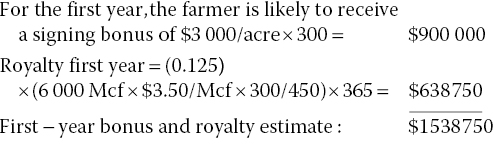
Table 13.2 Data for landowner royalty calculation.
| Natural gas royalty calculation | Rates |
| Signing bonus | $3000 per acre |
| Royalty rate | 12.5% |
| Average wellhead natural gas price | $3.50 per thousand cubic feet (Mcf) |
| Average well production rate (entire production unit) | 6 million cubic feet per day |
| Acres (owned by farmer) within the well production unit | 300 acres (121 ha) |
| Total number of acres within the well production unit | 450 acres (182 ha) |
The initial decline as measured in a decrease in gas production over the 12 months of operation of a Marcellus Shale well is key in estimating the potential for future production. First‐year gas production decline rates in Pennsylvania range from 60 to 80% (Figure 13.1). Unconventional production declines sharply, within the first few years, and then the gas production will level off or decline steadily but continue to produce for decades. Typical Marcellus Shale gas wells have an estimated lifetime of 20–30 years of production (Ladlee 2017).
Figure 13.1 Marcellus Shale gas production and decline curves
(Source: Modified after Ladlee (2017)).
13.2.5 Future Use
High‐volume hydraulic fracturing (HVHF) operations are an industrial process and may preclude or limit certain surface uses nearby by the surface rights owner. Examples of land use limitations might include residential, child day care, hospital, retirement homes, or other facilities where exposure to noise, windblown dust, or methane leakage can create a health risk. Once production is established and drilling and HVHF operations have been completed, surface use restrictions should be reevaluated by properly trained professionals.
13.2.6 Oil and Gas Production 2000–2015
The US Energy Information Administration (2016) has documented oil production in the United States. The new oil production has mainly been produced from black shales and other tight rocks in the Eagle Ford formation of south and east Texas, the Permian Basin of west Texas, and the Bakken and Three Forks formations of the Williston Basin in North Dakota and Montana. The increase in producing unconventional oil wells is mirrored in the number of producing unconventional gas wells with main production from black shales and other tight rocks in the following basins: 1) Marcellus and Utica formations of the Appalachian Basin, 2) the Bakken Formation in Williston Basin in North Dakota and Montana, 3) the Eagle Ford formation in east and south Texas, and 4) the stacked Permian Basin formations in Texas and New Mexico (US EIA 2016). There are 1.7 million active oil and gas wells that have been drilled since August 2015 in the United States (Kelso 2015). In the United States, as of 2013, more than 15.3 million people in 11 states live within 1 mile (1.6 km) of the hundreds of thousands of unconventional oil and gas wells drilled since 2000. Diagrams showing total crude oil production (Figure 13.2) and total natural gas production (Figure 13.3) from 2000 to 2015 show that in 2015, unconventional production methods represent 51 and 67% of the total production, respectively. Combined production figures from the same time period are summarized in Table 13.3.

Figure 13.2 Crude oil production from hydraulically fractured wells (US EIA 2016).

Figure 13.3 Natural gas production from hydraulically fractured wells (US EIA 2016).
Table 13.3 US crude oil and natural gas production (2000–2015).
Source: US EIA (2017), data from Drillinginfo and IHS Global Insight.
| Year | Number of hydraulically fractured wells | Oil production (bpd) | Percent from hydraulically fractured wells to total output (%) | Oil production (m 3 /d) |
| 2000 | 23 000 | 102 000 | <2 | 16 217 |
| 2015 | 330 000 | 4.3 million | 51 | 683 645 |
| Year | Number of hydraulically fractured wells | Gas production (Bcf/d) | Percent from hydraulically fractured wells to total output (%) | Gas production (m 3 /d) |
| 2000 | 26 000 | 3.6 billion | 7 | 101 million |
| 2015 | 300 000 | 53 billion | 67 | 1501 million |
Bcf/d, billion cubic feet per day natural gas; bpd, barrels per day crude oil; m3/d, cubic meters per day natural gas.
13.2.7 Value of Residential Real Estate
In general, residential property in close proximity to industrial activities is less valued than similar properties without those nearby uses. However, area‐wide increases in real estate value may relate to a shortage of housing supplies as well as the improving health of the local economy, greater local employment opportunities, and higher local and state revenues from operators and vendors. The sales comparison approach is the best method to determine residential real estate value (ILAC 2016). Income capitalization is often used for commercial property in conjunction with the sales comparison approach. The impacts of unconventional oil and gas production, if any, on residential real estate values should be determined by real estate experts in an unbiased and professional manner to objectively use the established appraisal valuation practices described in the Uniform Standards of Professional Appraisal Practices (Bell and Bell 2017). Real estate values relate to site‐specific conditions, and a licensed real estate appraiser should be contacted for detailed information.
13.2.8 Perceptions
In the popular press, in non‐peer‐reviewed articles about real estate prices in areas of unconventional oil and gas production, photos featuring flaming gases burning at the nozzle end of the kitchen faucet are common. Although the gas is likely methane, the sources for methane in water are numerous. Methane can be of biogenic origin, related to anaerobic decay of organic matter. Methane can also be naturally occurring in groundwater aquifers sourced from deeper coal seams or black shale units. Unconventional oil and gas production activities can also be a possible source of methane in tap water. In order to accurately confirm the source of methane in tap water, isotope geochemistry can be used to identify the origin of the dissolved methane. Nonetheless, photos of gas flames in tap water and thousands of articles, videos, and documentary films have created negative perceptions for real estate near unconventional drilling operations, regardless of the source of the methane.
Real estate values have a lot to do with perceived risks, and in one real estate study (Muehlenbachs et al. 2015a), the authors estimate home value declines in Pennsylvania from April 2011 to April 2012 in areas undergoing unconventional shale gas drilling and production. In the study, the authors noted that groundwater‐dependent homes may have large and negative local impacts on house prices in areas with unconventional oil and gas development. They argue that groundwater contamination can cause severe financial impacts to homeowners without the access to a piped water system. The number of homes with groundwater wells impacted by unconventional oil and gas production in the study area or nationally was not reported. At present, many of the unconventional oil and gas production areas tend to be rural. Rural houses next to or near gasoline stations, dry cleaners, cement plants, or other industrial facilities likewise may have similar potential risks of contaminated groundwater or industrial activities. The importance of the study (Muehlenbachs et al. 2015a) is that the perception by home buyers of the risk of possible contamination from unconventional oil and gas drilling and production, not the actual damages, impacts the home values (Table 13.4).
Table 13.4 Pennsylvania real estate.
Source: April 2011 to April 2012; from Muehlenbachs et al. (2015a).
| Proximity to shale gas well | Description | Loss in value |
| Very close: 0.9 miles (1.5 km) or closer | Perceptions of home buyers: significant groundwater contamination risk | −9.9 to −16.5% |
| Groundwater‐dependent homes | $30.167 average annual loss | |
| Homes with piped‐in water | $4802 average annual gain |
Rents in in economically booming Marcellus Shale gas area of Pennsylvania, as compared to New York which has a drilling moratorium (control area) vary dramatically over the spread of unobservable factors; the large effects were confined only to the higher rental market segments (Muehlenbachs et al. 2015b).
13.2.9 Property Value Survey
In a 2013 telephone survey of 550 homeowners in the Houston, Texas, area and the Alabama–Florida panhandle conducted by business researchers at the University of Denver (Throupe et al. 2013), a majority said they would decline to buy a home near a drilling site. The study also showed that homeowners bidding on similar homes near active unconventional oil and gas drilling and production locations reduced their hypothetical offers by 5–25%. Those surveyed were instructed to consider that they were going to be offered to bid on a home near unconventional oil and gas activities, including drilling, hydraulic fracture operations, and production. The authors described horizontal drilling, hydraulic fracturing methods, and production activities, as well as the potential risks of surface and subsurface impacts. Case studies of contamination claims were also discussed. Those surveyed by telephone were also provided a summary of federal and state disclosure regulations and management requirements for the oil and gas field operators.
The surveyed Texans, generally more comfortable with the oil and gas industry, discounted their real estate bids by about 6%. From the panhandle of Florida to southern Alabama, where the oil and gas industry is not as popular as in Texas, the real estate bids were reduced by 2.5 times the Texan amount, to about 15%. The importance of the study (Throupe et al. 2013) is that it shows the variations in comfort level of homeowners with the oil and gas industry operations, which reflects the perceptions of the risks of hydraulic fracturing operations in two different populations.
13.2.10 Home Prices near Well Sites
A 2010 real estate study (IRR 2010) was conducted using four criteria in the town of Flower Mound, Denton County, Texas. The study area lies within the Barnett Shale area where unconventional drilling and production of natural gas has been ongoing and is located in the Lewisville–Flower Mound real estate submarket, northwest of the Dallas–Fort Worth International Airport, about 28 miles (45 km) northeast of Dallas and 25 miles (40 km) northeast of Fort Worth, Texas (IRR 2010). Home prices near well sites in the Lewisville–Flower Mound real estate submarket are summarized in Table 13.5.
Table 13.5 Town of Flower Mound, Texas, and home prices near well sites.
Source: From IRR (2010).
| Criteria | Description | Data | Comments |
| Price–distance relationship | Sales price of houses on $ per square foot compared with distance to well site in feet | Linear trend developed and relationship noted | Sales of houses outside ½ mile (0.8 km) were used for comparison |
| Comparable sales analysis | Sales adjacent to well sites compared with four comparable properties | Actual sales price of house adjacent to well is compared with estimated value of same house not adjacent to well site | Sales of houses outside ½ mile (0.8 km) were used for comparison, where possible |
| Statistical analysis | Analysis of all sales with a comparison of distance from well site | To isolate the influence of home prices to proximity to well sites, linear regression analysis was performed | Estimate of the influence on home prices and estimate of statistical significance of the distance to the well site |
| Survey of market participants | Interview real estate agents in locale and surrounding area | Determine whether buyers considered home price related to the proximity to well sites | Evaluate pricing criteria for homes next to well sites for marketing purposes |
Conclusions from the study (IRR 2010) can be made regarding home values relating to the proximity to well sites:
- Many study participants believe the proximity of unconventional gas wells negatively impact home values.
- The prices of upscale homes are affected more significantly by the proximity to well sites than lower priced homes.
- Homes with small lots such as patio homes or zero lot line properties are less likely to be impacted in price than homes on larger lots.
- The largest price impacts are to houses immediately adjacent to a well site.
- The only property subset to be negatively impacted were houses valued higher than $250 000:
- The value of properties in this category were negatively impacted about −3 to −14% of total value.
- The range of property value decline found in price–distance relationships was about −2 to −7%.
- No statistically significant diminution in value was noted using statistical regression methods.
- Values of upscales homes adjacent to well sites or within 700 ft (213 m) of the wellhead were impacted.
- Visual and sound buffers such as vegetation, other houses, or sufficient distance greatly reduces impact on home values.
- Without buffers between the home and well site, the negative proximity effect disappears at around 1000 ft (305 m) distance.
- After the drill rig is removed, hydraulic fracture operations have ceased, and gas production is ongoing, the negative impacts on home prices decrease with time.
- Once wells or gas compressors with sound‐deadening containment structures are producing, no discernable difference in home values was noted.
Notes: No homes in the Flower Mound, Texas, study area were closer than 1000 ft (305 m) to soundproofed compressor stations.
The conclusions of the Texas study (IRR 2010) noted that in general, once the drill rigs and fluid tanks, the most obvious aspects of gas operations, are removed from the well pads, the negative impacts on home values are significantly reduced with no discernable differences in house prices between homes proximal to producing wells and those further away.
Differences in home values related to proximity to wellheads, compressor stations, pipelines, or other facilities may vary with region and home‐specific circumstances.
13.3 Water Supplies
13.3.1 Domestic Water Well Costs
Although it is unlikely that large‐scale groundwater impacts will occur related to a particular well pad spill or specific hydraulic fracturing chemical injection at an unconventional oil or gas well, domestic water wells can certainly be impacted by industrial activities. Depending on the size of the spill or injection and the characteristics of the chemicals released into the environment, as well as the subsurface conditions and the effectiveness of the emergency responders, a release is likely to be limited to one or a few domestic wells near the well pad. Other large sources of potential leaks related to unconventional oil and gas activities, such as pipeline breaks or railcar spills, can also have a large radius of impact and can contaminate domestic water wells.
Poor groundwater quality in many rural areas is not necessarily related to unconventional oil and gas operations. Natural conditions in aquifers or conditions of domestic water wells change over time and should be tested and compared with water quality standards. If unconventional oil and gas activities are suspected of contributing to water quality degradation in a domestic well, geochemical studies using isotope analysis and chemical ratios among other tests can be used to confirm the sources of impacts.
The replacement of impacted domestic water wells can cost a few thousand dollars to tens of thousands of dollars, depending on market conditions in the area where the drilling is proposed, site‐specific access issues, target depth, well casing diameter, cost of supplies at the time of installation, variations in permit fees, and other variables. Well plugging of the impacted well should also be factored into the cost of well replacement. For new domestic water wells, the contractor should test the well for its well‐sustained water yield (gallons per minute or liters per minute) to estimate the quality of the well. The water depth or drawdown during the pump test should be recorded as well as the time it takes for the water level to recover back to pretest levels. The well should be sampled for water quality parameters and disinfected. A professional geologist or professional engineer with expertise in hydrogeology should design the water well to optimize well performance. A checklist for well installation and maintenance (see Table 13.6 , Appendix I) provides suggestions on inspections and maintenance for well owners. Domestic well installation costs are estimated based on depth and other factors (Table 13.7).
Table 13.7 Estimate of the range of costs ($2017) for domestic well installation.
| Range of costs $2017 | 4‐in‐diameter well (10 cm) | 6‐in‐diameter well (15 cm) |
| Cost per foota ($) | 25–35 | 30–40 |
| Well depth | Estimate | |
| 200 ft (61 m) ($) | 5 000–7 000 | 6 000–8 000 |
| 500 ft (152 m) ($) | 12 500–17 500 | 15 000–20 000 |
| 1000 ft (305 m) ($) | 25 000–35 000 | 30 000–40 000 |
| 2000 ft. (610 m) ($) | 50 000–70 000 | 60 000–80 000 |
| Extremely difficult access or geologic conditions (add surcharge) ($) | 5–25 per footsurcharge | |
| Example of other costs | Estimate | |
| Submersible pump or other pump system ($) | 3 000–7 500+ | |
| Storage tank, piping, water line to house | Site specific, budget $5 000–7 500+ | |
| Other costs: permits, well surveying, if needed, etc. | Site specific, budget $1 000–3 500+ | |
| Water treatment, if needed | $1 000–15 000+ depending on treatment | |
| Well plugging or abandonment of impacted domestic water well, disposal of wastes | Site specific, budget $2 000–12 500+ | |
Various sources of contractor costs were used, including the National Groundwater Association 2016 NGWA Contractors Survey (NGWA 2016) and CostHelper (2017).
13.3.2 Public Water Supplies
Regardless of the source of degraded water quality, connecting into a city or other municipal water supply or public water system may be one way to mitigate impacted domestic wells. A public water system, as defined by the US Safe Drinking Water Act (SDWA), provides potable water for human consumption through a piping system. The system has to have (i) at least 15 service connections or (ii) serves an average of at least 25 people for at least 60 days annually. A public water supply can be a large production well with water treatment system, or other sources of water can be utilized. Both municipal and public water supplies have requirements for analytical testing and reporting. In areas where a municipal or a public water supply is available, general estimated connection costs are listed in Table 13.8.
Table 13.8 Estimated costs (2017) for water supplies.
Site‐specific costs will vary.
| Water line | Estimated low cost $2017 ($) | Estimated high cost $2017 ($) |
| Water lines PVC | <4 per feet | 10 per feet |
| Small excavator to trench: daily rental | 500 per day | 2500 per day |
| Additional supplies | 500 | 3500 |
| Contractors: laborers, supervisors, etc. | 50 per hour per person | 100 per hour per person |
| Municipal water hook‐up fee | <1000 | 5000+ |
| Oversight by licensed professional | 500 | 5000+ |
13.3.3 Water Treatment Systems
Water sampling and analysis of the well water and tap water is necessary to identify whether water quality is acceptable or if water treatment is necessary. Small water treatment systems are available and should be properly sized based on water flow and contaminant load based on the laboratory analysis. The system should be designed to include enough treatment media to prevent contaminant breakthrough for a specific amount of time and flow. Water treatment systems require maintenance and cleaning or replacing consumable media filters. Regular laboratory analysis is recommended to monitor the contaminant load. Estimated costs for water treatment systems (Table 13.9) vary greatly.
Table 13.9 Estimated costs for small domestic to large municipal water treatment systems.
| Small water treatment system for house | Estimated low cost $2017 ($) | Estimated high cost $2017 ($) |
| Laboratory analysis to test tap water and well water | 250 | 1500 |
| Filtration system (sediment filter, granular activated carbon filter, post carbon filter) | 200 | 1250 |
| Storage tank | 500 | 2500 |
| Water softener | 500 | 2500 |
| Reverse osmosis membrane | 200 | 1500 |
| Disinfection unit (ozone) | 100 | 750 |
| Disinfection unit (ultraviolet) | 500 | 2000 |
| Acid neutralization | 500 | 1500 |
| Air injection units to remove iron, sulfur, and manganese | 500 | 2000 |
| System design and installation | 500 | 1000 |
| Small‐scale water treatment facilities can be designed for under $50 000 but can cost well over $500 000 for neighborhood water treatment systems. Larger municipal water treatment systems are multi‐million‐dollar capital improvement projects | ||
| Water treatment system | Estimated low cost $2017 ($) | Estimated high cost $2017 ($) |
| Small neighborhood water treatment system | 150 000 | >500 000 |
| Municipal water treatment system | 1 million to 10+ million | 50 million to >100+ million |
| Larger water treatment systems typically use many of these processes: | ||
| General treatment sequence | Description | |
| Preliminary treatment | Removal of debris, grit, suspended sediment, and turbidity | |
| Coagulation and flocculation | Get larger particles to bind together using additives (alum) | |
| Sedimentation basin | Floc particles settle out of water and into basin | |
| Softening and stabilization | Aeration for removal of iron, hydrogen sulfur, and manganese | |
| Filtration | Sand, granular activated carbon (GAC), and gravel to filter the water | |
| Disinfection | Chlorine, ultraviolet (UV) light, ozone, or reverse osmosis membranes to remove pathogens and disinfect water | |
| Public health additives | Fluoridation at low levels to prevent tooth decay | |
| Tower or storage tank | Water storage for future use | |
| Pumps | Distribute water into system | |
| Other chemical additives | Corrosion control using a phosphorus compound to reduce pipe corrosion and chloramine (chlorine and ammonia) for biological pathogens | |
13.4 Other Mitigating Costs
13.4.1 Soundproofing Equipment Shed
Soundproofing of sheds containing industrial equipment reduces noise levels (Table 13.10).
Table 13.10 Estimated costs for soundproofing equipment sheds.
| Soundproofing equipment sheds | Estimated low cost $2017 ($) | Estimated high cost $2017 ($) |
| Insulation and soundproofing panels (depends on size of shed and sound levels) | 2 000 | 10 000 |
13.4.2 Road Construction Projects
Unconventional oil and gas development requires building new roads to the well pads. Damage to roads is affected by many factors, including age of road, truck weight and type, traffic patterns, road construction material, road subbase, drainage, environmental conditions, and other factors.
13.4.2.1 Truck Trip Estimates
An approach used for evaluating truck trips to unconventional oil and gas operation sites relies on understanding the effects of weight loads on roadway pavement and to express all truck loads as equivalent single axle loads (ESAL). For a variety of different roadway types, vehicle weights, and axle combinations, the load equivalency factor (LEF) is the way of estimating roadway damage caused by a single pass of each vehicle relative to the damage per single pass of an ESAL (Abramzon et al. 2014). An estimate of the number of truck trips to unconventional gas sites in Pennsylvania for each operation is summarized in Table 13.11. A study on New York HVHF data is presented in Table 13.12.
Table 13.11 Assumed heavy truck trips used for the construction and operations of a single unconventional gas well in Pennsylvania.
Source: From Abramzon et al. (2014).
| Well pad activity | High range: number of heavy truck trips for early well pad development | Low range: number of heavy truck trips for peak well pad development |
| Drill pad construction (worker and supply transportation) | 45 | 45 |
| Rig delivery | 95 | 95 |
| Drilling fluids delivery | 45 | 45 |
| Non‐rig drilling equipment | 45 | 45 |
| Drilling (worker transportation) | 50 | 50 |
| Completion chemical delivery | 20 | 20 |
| Completion equipment delivery | 5 | 5 |
| Hydraulic fracturing equipment (trucks and tanks) | 175 | 175 |
| Hydraulic fracturing water hauling | 500 | 60 |
| Hydraulic fracturing sand delivery | 23 | 23 |
| Produced water disposal | 100 | 17 |
| Final pad prep activities (worker transportation) | 45 | 45 |
| Miscellaneous | 12 | 5 |
| Total one‐way, loaded heavy truck trips per well | 1160 | 630 |
Table 13.12 Examined truck trips per HVHF well and multiple wells.
| Description | Truck trips | Additional truck trips to haul equipment, materials, and workers | Maximum number of truck trips | Study |
| Single HVHF well | 3 000 | 220–364 | 3 364 | Moss (2008)a |
| 1 760–1 904 | 1 904 | Podulka and Podulka (2010) | ||
| 1 800–2 600 | 2 600 | NY SEIGC (2011) | ||
| 8 HVHF wells | 14 400–20 800 | 20 800 | NY SGEIS (2011) | |
a Moss (2008) describes the potential development of the natural gas resources in the Marcellus Shale for New York, Pennsylvania, West Virginia, and Ohio as part of a National Park Service, US Department of the Interior study. The other studies estimated potential truck trips for unconventional gas extraction in New York.
13.4.2.2 Cost of Road Construction
The cost per mile of roadway depends on a variety of factors:
- Topography along road.
- Area economics (expensive versus lower cost).
- Access to area.
- Available labor and equipment.
- Conditions (urban versus rural).
- Terrain (mountainous versus flat).
- Climate.
- Type of road construction.
- Length of roadway.
- Width of roadway.
- Anticipated traffic.
- Weight of vehicles.
- Durability of construction materials.
- Underlying geology.
- Geotechnical stability.
- Stormwater control and number of culverts.
- Number of special structures such as bridges or tunnels.
A general range of estimates for roadway construction and repair (Table 13.13) varies.
Table 13.13 Range in price for new road construction and repair per mile (1.6 km).
Source: Data from Elswick (2016).
| New road construction | Low estimate ($2017) | High estimate ($2017) |
| Rural or suburban area construction; 2 lane, undivided | $2 million per mile | $3 million per mile |
| Urban area construction; 2 lane, undivided | $3 million per mile | $5 million per mile |
| Road repair | ||
| Mill and resurface 4‐lane road | $1.25 million per mile |
Costs per mile in Pennsylvania (Table 13.14) show variations in design life. Most of the roadways associated with shale gas are on roads not part of the national highway system. Consumptive road use and cost per lane mile driven by trucks used for the construction and operation of Pennsylvania shale gas wells (Table 13.15) show a 2017 cost ranging from $337 to 621 cost per lane per mile for each HVHF well. Cumulative estimates on a state scale indicate that road destruction or reduction in the useful life of roads related to unconventional oil and gas operations is significant (Table 13.16).
Table 13.14 Characteristics of roads assumed to be used for construction and operation of shale gas wells in Pennsylvania.
Source: From Abramzon et al. (2014).
| PennDOT road maintenance class | A | B | C | D | E |
| Assumed description | Interstate | NHS | NHS | Non‐NHS > 2000 ADT | Non‐NHS < 2000 ADT |
| Design pavement life in EASLs | 65 000 000 | 25 000 000 | 25 000 000 | 21 000 000 | 6 000 000 |
| Lane mile reconstruction costs ($2012) ($) | 3 175 182 | 2 684 367 | 2 684 367 | 2 571 398 | 2 333 664 |
| Lane mile reconstruction costs ($2017) ($) | 3 397 445 | 2 872 273 | 2 872 273 | 2 751 396 | 2 497 020 |
| Average distribution of shale gas activity VMT (%) | 2 | 2 | 22 | 46 | 28 |
Originally calculated in 2012 US dollars, updated to 2017 US dollars (6.9% cumulate rate of inflation).
Road types:
- Interstate.
- NHS = National Highway System Interstate.
- NHS = Non‐interstate.
- Non‐NHS > 2000 average daily traffic (ADT).
- Non‐NHS < 2000 average daily traffic (ADT).
Table 13.15 Estimated consumptive road use and costs per lane mile driven by trucks used for the construction and operation of shale gas wells in Pennsylvania.
Source: From Abramzon et al. (2014).
| Road class | A | B | C | D | E | Total | |
| Low truck trip range | Consumptive roadway use per well (%) | 0.0001 | 0.0001 | 0.0015 | 0.0036 | 0.0077 | |
| Damage costs per lane mile for each well; $2012 ($) | 2 | 3 | 40 | 92 | 180 | 315 | |
| $2017 ($) | 2 | 3 | 43 | 98 | 105 | 337 | |
| High truck trip range | Consumptive roadway use per well (%) | 0.0001 | 0.0002 | 0.0027 | 0.0066 | 0.0142 | |
| Damage costs per lane mile for each well; $2012 ($) | 3 | 5 | 72 | 168 | 331 | 580 | |
| $2017 ($) | 3 | 5 | 77 | 180 | 354 | 621 |
Originally calculated in 2012 US dollars, updated to 2017 US dollars (6.9% cumulate rate of inflation).
Table 13.16 Costs for road degradation based on a state or regional scale. For larger road degradation studies on a state scale, the costs are in hundreds of millions of dollars.
Source: Based on Ritzel (2015).
| State | Cost in study ($) | Cost $2017a ($) | Description | Study |
| Pennsylvania, Dept. of Transportation (PDOT) | 265 million | 283 million | Road damage due to drilling in Marcellus | Christie (2010) and Dutzik et al. (2012) |
| North Dakota | 1 billion | 1 billion | Infrastructure, primarily for roads damaged by heavy energy‐related truck traffic | Gunderson (2012) and White (2013) |
| Arkansas | 450 million | 474 million | Road damage due to HVHF truck traffic | Heinberg (2013) and Rogers (2013) |
| New York | 378 million | 413 million | Road maintenance costs to mitigate impacts from trucks servicing 40 000 proposed HVHF wells | NY SGEIS (2011) |
| Texas Department of Transportation (TDOT) | 4 billion | 4 billion | Cost of maintaining roadway infrastructure degraded by servicing HVHF wells | Heinberg (2013) and Rogers (2013) |
For larger road degradation studies on a state scale, the costs are in hundreds of millions of dollars.
a 6.9% cumulative rate of inflation, for example, 2012–2017.
13.5 Mitigation of Subsurface Impacts
13.5.1 Orphan Well Survey
Orphan wells can be located using a variety of techniques. Estimated costs for locating one or two wells on one or two acres of accessible, vacant land in a relatively level rural area is summarized in Table 13.17.
Table 13.17 Estimated costs for locating orphan wells.
| Orphan well survey | Estimated low cost $2017 ($) | Estimated high cost $2017 ($) |
| Locate wells from historic documents, building department files, well permits, historic aerials, investigating local well driller files, etc. | 500 | 3500 |
| Oversight by licensed professional | 500 | 1000 |
| Site inspection with ground‐penetrating radar (GPR) and magnetic tools | 1000 | 3500 |
| Total | 2000 | 8000 |
13.5.2 Orphan Well Destruction
Protecting groundwater resources by sealing off surface or subsurface contamination of oil and gas activities, salt water, or poor quality water zones is the primary objective of proper well destruction. Orphan wells, which include permanently inactive oil, gas, water, and dewatering wells, are unplugged and abandoned and can create subsurface conduits for contaminants to migrate. Due to the potential of compromised well integrity, gases and fluids can be conveyed up or down orphan wells and impact drinking water sources. Variations in well destruction methods exist between different agencies. A general diagram for properly destroyed wells (Figure 13.4) shows the California Department of Water Resources approach toward destroying orphan wells (DWR 1981).

Figure 13.4 General diagram showing properly destroyed wells
(Source: Modified after DWR (1981)).
Pennsylvania has countless abandoned historic oil and gas wells, and the 1999 Environmental Good Samaritan Act protects landowners, groups, and individuals who volunteer to perform environmental restoration projects from civil and environmental liability. This law is intended to encourage landowners and others to plug and destroy orphan oil and gas wells and abate the associated water contamination. The act also covers volunteer actions caused by abandoned mining operations, including coal mines, which can cause acid mine drainage (PDEP 2017). Estimated costs for properly destroying orphan wells are summarized in Table 13.18.
Table 13.18 Cost for destroying orphan wells.
| Task | Depth | Estimated low cost $2017 ($) | Estimated high cost $2017 ($) |
| Destroy orphan wells | Up to 3000 ft (914 m) | <20 000 | 50 000 |
The range of well destruction costs relate to many variables, including:
- Availability of drilling rigs.
- Depth to the bottom of the well.
- Well diameter.
- Well fluids (oil, gas, water, etc.).
- Obstructions in well.
- Weight and size of downhole pump, if present.
- Access to well site.
- Type of well construction.
- Regulatory agency requirements.
- Cost of permits.
- Area economics (expensive versus lower cost).
- Cost of professional oversight.
13.5.3 Subsurface Investigations
A Phase II Subsurface Investigation is used to collect soil, soil vapor, and groundwater samples. If the investigation relates to surface leaks or spills, the investigation typically starts evaluating conditions at shallow depths. For larger releases, the study area might enlarge from the known contamination source area and move toward areas with possible exposure pathways, toward areas with lower surface topography, in the direction of shallow groundwater flow, or toward areas having subsurface utilities or other conduits.
The general costs listed below are for an initial one day of soil, soil vapor, or groundwater sampling with a direct push technology (DPT) or probe rig with a probe operator and geologist or engineer supervision (Table 13.19). Shallow groundwater monitoring well installation is usually performed using a hollow stem auger rig. Variations in costs exist for rig rates, professional service hourly rates, permit charges, laboratory fees, and other costs, depending on local conditions.
Table 13.19 Estimated costs for subsurface investigations and samplinga.
| Phase II Subsurface Investigation | Estimated low cost $2017 a ($) | Estimated high cost $2017 a ($) |
| Direct push rig sampling: one‐day sample to 30 ft (9 m) | 2000 | 3 000 |
| Work plan stamped by licensed professional | 500 | 3 500 |
| Drilling permits | No charge | 1 500 |
| Laboratory budget | 500 | 2 500 |
| Professional services | 2000 | 5 500 |
| Total Phase II Subsurface Investigation | 5000 | 16 000 |
| Groundwater monitoring well installation | ||
| Cost of installing 3 monitoring wells to 30 ft (10 m) | 20 000 | 30 000 |
| Regulatory discussions, soil disposal, other costs | 10 000 | 15 000 |
| Four quarters of sampling, laboratory costs, reporting (price per year) | 10 000 | 20 000 |
| Well destruction (three wells) by overdrilling, permitting, final well destruction report | 15 000 | 25 000 |
| Well destruction (three wells) by pressure grouting, permitting, final well destruction report | 10 000 | 15 000 |
a Site‐specific prices vary with contractor availability, local regulatory requirements, laboratory costs, professional service hourly rates, etc. ($ year = in 2017 year dollars)
13.5.4 Hypothetical Case: Suspected Pipeline Spill Project
In a hypothetical case, a suspected Bakken crude oil pipeline spill was called in by an anonymous source to have occurred near Fort Madison, Iowa. An inspection by the pipeline operator revealed only spray paint graffiti and no obvious pipeline spill or release. Neighbors were concerned about the vandalism. To be safe, the insurance carrier for the pipeline operator contacted ACME Consulting Co. to inspect and sample the soil with a hand auger by collecting 10 samples in the vicinity of the pipeline in the area of the alleged incident. The insurance carrier asked for 10 discrete soil samples to be analyzed and to run for only total petroleum hydrocarbons (TPH) and volatile organic compounds (VOCs). Carol Rockhammer, a principal geologist at ACME Consulting, was assigned the project and made a scope of work to include:
- Develop a site‐specific health and safety plan.
- Prepare a brief written work plan of field activities, sampling and safety supplies, air or soil monitoring equipment, laboratory analysis, participating staff, schedule, etc.
- Direct the staff geologist or engineer to inspect the site, make a map of area, take photos, interview the pipeline manager (if available), collect 10 soil samples at random depths, and prepare field notes and the laboratory chain of custody forms.
- Authorize laboratory to analyze the samples for TPH by US EPA Method 8015M by gas chromatography–flame ionization detector (GC‐FID) and VOCs by US EPA Method 8260B by gas chromatography–mass spectroscopy (GC‐MS).
- Prepare a report stamped by a licensed geologist or engineer with sampling maps, photos, laboratory reports, chain of custody form, and the findings.
13.5.4.1 Cost of Hypothetical Soil Sampling Project
Planning field budgets vary in different areas, but the overall hourly rates provide a guide to the level of cost for an environmental sampling project (Table 13.20). The hypothetical one‐day hand auger soil sampling project near the Bakken crude oil pipeline requires the cost of a staff geologist or engineer in the field for eight hours, two hours of principal‐level oversight, a lab cost of about $3000 and report preparation of about eight hours of a staff geologist or engineer, two hours of computer‐aided design (CAD) drafting of the figures, and two hours for administrative support. Other costs (Table 13.21) include a vehicle and equipment rental.
Table 13.20 General costs for an environmental sampling project (10 samples).
| Professional staff title/classification | Estimated low cost $2017 ($ per hour) | Estimated high cost $2017 ($ per hour) | Number of hours | Amount (assume average $ per hour cost) |
| Principal engineer/geologist (licensed) | 150 | 250 | 2.00 | 400 |
| Project manager | 125 | 195 | 1.00 | 160 |
| Senior engineer/geologist | 105 | 150 | 0 | 0 |
| Project/associate engineer/geologist | 95 | 125 | 0 | 0 |
| Staff engineer/geologist | 85 | 105 | 16 | 1520 |
| Senior technician | 75 | 95 | 0 | 0 |
| Technician | 65 | 85 | 0 | 0 |
| Drafts person | 105 | 125 | 2.00 | 230 |
| Administrative support | 55 | 75 | 2.00 | 130 |
| Vehicle for the day | 75 | 125 | 1 | 100 |
| Hand auger kit, supplies (sample tubes, cooler, ice, labels, nitrile gloves, etc.) | 50 | 100 | 1 | 75 |
| Laboratory: TPH: EPA 8015M (GC‐FID) | 75 | 125 | 10 | 1000 |
| Laboratory: VOCs: EPA 8260B (GC‐MS) | 175 | 225 | 10 | 2000 |
| Total project cost ($) | 5615 | |||
Table 13.21 Costs of other services.
| Scope of work | Estimated low cost $2017 ($ per hour) | Estimated high cost $2017 ($ per hour) |
| Example work plans (define scope of work) | ||
| Preliminary site assessment work plan | 2 000 | 5 000+ |
| Soil and water subsurface investigation work plan | 3 500 | 10 000+ |
| Interim remediation action plan (IRAP) | 3 500 | 10 000+ |
| Health and safety plan (HSP) | 2 500 | 7 500+ |
| Example field investigation projects and report preparation | ||
| Trench pit or excavation: for 50 ft (15 m) to a depth of 15 ft (5 m) | 10 500 | 15 500+ |
| Cone penetrometer test (CPT): 10 CPT probes to 30 ft (9 m), permits, soil and water samples, laboratory analysis, and report preparation | 25 000 | 35 000+ |
| Soil boring project: 4 soil borings to 30 ft (9 m), permitting, geologist/engineer, driller, laboratory, and reporting | 16 500 | 23 500+ |
| Soil boring project: 8 soil borings to 50 ft (15 m), permitting, geologist/engineer, driller, laboratory, and report preparation | 39 500 | 45 000+ |
| Groundwater sampling: (10) grab groundwater samples to 30 ft (9 m), laboratory, report preparation | 17 750 | 24 500+ |
| Groundwater well installation: (3) borings drilled to 30 ft (9 m) and converted into 2 in (5 cm) PVC monitoring wells, laboratory, drums, disposal, and report preparation | 19 000 | 29 500+ |
| Groundwater well development | 1 500 | 3 000+ |
| Soil vapor test: field activity, laboratory, report preparation | 8 500 | 12 500+ |
| Water well pump test: (two day), data loggers, report preparation, water storage and disposal | 19 000 | 25 500+ |
| Groundwater monitoring event: (3) wells to 30 ft (9 m), low flow groundwater sampling, laboratory, disposal, report preparation | 5 000 | 7 500+ |
| Groundwater monitoring event: (6) wells to 50 ft (15 m), low flow groundwater sampling, laboratory, disposal, report preparation | 8 000 | 10 500+ |
| Technical documents | ||
| Corrective action plan (CAP) | 10 000 | 15 000+ |
| Remedial action plan (RAP) | 12 000 | 17 500+ |
| Site conceptual model report | 5 000 | 15 000+ |
a Costs are for planning purposes only and vary with specific project location, access, site complexity, regulatory agency requirements, and other factors.
13.6 Remediation Strategies
There are many considerations in selecting a remedial technology:
- Space requirements.
- Time constraints.
- Regulatory acceptance.
- Technical considerations.
- Groundwater depth.
- Soil types.
- Contaminant characteristics.
- Consultant specifications.
- Landowner needs.
- Tenant needs.
- Potential long‐term liability.
- Future site use.
- Cost and timing of construction payments.
- Funding sources (banks, loans, US EPA, etc.).
- Financing issues.
- Interest rates.
- Loan terms.
- Tax and accounting implications.
- Price of clean land.
- Deed restrictions.
- Stigma devaluation.
- Others.
SMART Process
In planning remediation projects, the SMART process provides the recommendation to identify the criteria for case closure:
- Specific objectives
- Measurable goals
- Agreement
- Realistic expectations
- Time bound
13.6.1 Risk Management Strategies
The boom‐and‐bust economic cycle in the oil and gas business has created situations where a variety of owners or parties may end up as the responsible party in charge of environmental cleanups or maintenance and repair of aging facilities. Those potentially responsible parties may include operators working on environmental cleanup projects, lenders associated with a foreclosed property where production profits were less than the loan payments, or public agencies taking over remediation obligations from bankrupt companies. As the economics of the unconventional oil and gas fields decline, larger oil and gas companies will likely sell off marginally producing properties to smaller companies or even individuals with less financial resources. In bust cycles, the potential for facility abandonment into orphan sites becomes greater.
13.6.2 Lender Risk Reduction
Banks or private lenders can be involved with underwriting and funding unconventional oil and gas production. There are four ways lenders can better address environmental liabilities and associated financial risks of environmentally impacted properties or properties that require ongoing maintenance and repair:
- Risk avoidance: Stay away from prospect to eliminate or lower risk.
- Risk reduction: Hire better consultants, use better risk management tools, acquire more data, make better decisions, and provide more training to staff reviewing lending opportunities.
- Risk sharing: Transfer or outsource the risks by bringing in other partners, or use insurance to address worst‐case scenarios.
- Risk retention: Accept the risk and budget for the failures by increasing interest rates and fees to cover uncertainties.
13.6.3 Green and Sustainable Remediation
After decades of cleanups that included excavating soils contaminated with low‐level petroleum hydrocarbons and transporting the impacted soil for redeposition in landfills, regulators, consultants, responsible parties, and others decided to evaluate the environmental impacts of the remedial activities themselves (fuel consumption, vehicle exhaust, noise, water consumption for dust control, traffic, etc.) and the entire environmental regulatory decision‐making process (DTSC 2009). The main concept of green remediation is to obtain optimal sustainable revitalization in a project by striving for balance between environmental, economic, and social aspects (DTSC 2009). The evaluation included reviewing the life cycle of activities and the wastes occurring within the process (Figure 13.5). Instead of working with a specific contaminant concentration as a cleanup goal to a spill, a life cycle evaluation framework can be designed by regulators and responsible parties and the community to include other impacts such as ecosystem, or global warming effects, for example (Figure 13.6). For the green and sustainable remediation approach to site cleanup the environmental impacts of site remediation projects are considered as well as economics, effectiveness, and the likelihood of success. A Green Remediation Evaluation Matrix (GREM) was developed for evaluating one cleanup technology or approach compared with remedial alternatives (Table 13.22). A checklist (see Table 13.23, Appendix I) was developed for environmental stressors of remediation by DTSC (2009). As applicable, some of the same environmental impacts (soil disturbance, noise, odor, vibration, air pollution, traffic, etc.) on the environmental remediation checklist may apply to the original unconventional oil and gas drilling and HVHF operations.
Figure 13.5 A schematic showing the process from raw materials to product production to cleanup activities and the potential environmental impacts
(Source: Modified after DTSC (2009)).

Figure 13.6 Diagram showing life cycle framework of resources including inputs (raw materials and resources), remedial technologies, and transportation of products and wastes, outputs, and large‐scale impacts (DTSC 2009).
Table 13.22 Green Remediation Evaluation Matrix Checklist (GREM) (DTSC 2009).
Source: From DTSC (2009).
| Stressors | Affected media | Mechanism/effect | Yes or Noa | Score |
| Substance release/production | ||||
| Airborne NOx and SOx | Air | Acid rain photochemical smog | ||
| Chlorofluorocarbon vapors | Air | Ozone depletion | ||
| Greenhouse gas emissions | Air | Atmospheric warming | ||
| Airborne particulates/toxic vapors/gases/water vapor | Air | General air pollution/toxic air/humidity increase | ||
| Liquid waste production | Water | Water toxicity/sediment toxicity/sediment | ||
| Solid waste production | Land | Land use/toxicity | ||
| Thermal releases | ||||
| Warm water | Water | Habitat warming | ||
| Warm vapor | Air | Atmospheric humidity | ||
| Physical disturbances/disruptions | ||||
| Soil structure disruption | Land | Habitat destruction/soil Infertility | ||
| Noise/odor/vibration/aesthetics | General environment | Nuisance and safety | ||
| Traffic | Land; general environment | Nuisance and safety | ||
| Land stagnation | Land; general environment | Remediation time; cleanup efficiency; redevelopment | ||
| Resource depletion/gain (recycling) | ||||
| Petroleum (energy) | Subsurface | Consumption | ||
| Mineral | Subsurface | Consumption | ||
| Construction materials (soil/concrete/plastic) | Land | Consumption/reuse | ||
| Land and space | Land | Impoundment/reuse | ||
| Surface water and groundwater | Water, land (subsidence) | Impoundment/sequester/reuse | ||
| Biology resources (plants/trees/animals/microorganisms) | Air, water, land/forest, subsurface | Species disappearance/diversity reduction regenerative ability reduction | ||
Each GREM Checklist is designed to be used per one technology or remedial alternative.
a Please note whether the impact applies or does not apply to the alternative and continue GREM Checklist evaluation process.
13.6.3.1 Green and Sustainable Remediation Tools and Software
Numerous remediation optimization and costing tools and spreadsheets are available to evaluate sustainable approaches to soil and groundwater cleanup (US EPA 2017). A few selected tools are listed below.
13.6.3.2 SiteWise™ Tool for Green and Sustainable Remediation
For green and sustainable remediation, SiteWise is an Excel‐based remediation technology selection and optimization tool for a variety of contaminants, developed by the Department of the Navy, Army Corps of Engineers, and Battelle. The SiteWise Green and Sustainable Remediation tool can help users evaluate the following quantifiable metrics in a cleanup project:
- Energy consumption
- Greenhouse gas (GHG) emissions
- Criteria pollutant emissions
- Water impacts
- Ecological impacts
- Resource consumption/waste generation
- Worker safety
- Community impacts
13.6.3.3 Sustainable Remediation Tool (SRT)
The Air Force Center for Engineering and the Environment (AFCEE) and partners have developed the Sustainable Remediation Tool (SRT) to help with (i) planning for future implementation of cleanup technologies and (ii) evaluating remediation system optimization that are already in place or comparing remediation approaches using sustainability metrics. The user can compare SRT sustainability metrics for the following remedial methods: excavation, soil vapor extraction, pump and treat, and enhanced in situ biodegradation.
13.6.4 Natural Attenuation Software (NAS)
Although rapid natural attenuation, the biological and abiotic degradation of contaminants in the environment, does occur when conditions and biochemistry are optimal, frequently, oxygen or other limiting factors exist, which preclude rapid natural attenuation. Nonetheless, Natural Attenuation Software (NAS) is a screening tool to estimate remediation time frames for monitored natural attenuation (MNA) to reduce groundwater contaminant concentrations to regulatory agency approved limits and to assist stakeholders in decision‐making on the level of source zone treatment in conjunction with MNA using site‐specific remediation objectives. According to US EPA (2017), NAS is designed for application to groundwater systems that have porous, relatively homogeneous saturated sands and gravels. The software assumes that groundwater flow is uniform and unidirectional. NAS consists of a combination of analytical and numerical solute transport models. Natural attenuation processes as reflected in the NAS models include advection, dispersion, sorption, nonaqueous phase liquid (NAPL) dissolution, and biodegradation. The software determines redox zonation and estimates and applies varied biodegradation rates from one redox zone to the next (US EPA 2017).
13.6.5 Mass Flux Toolkit
The Mass Flux Toolkit was developed for the Department of Defense ESTCP program. It is a simple software tool for users to learn about different mass flux approaches, calculate mass flux from transect data, and apply mass flux values to optimize groundwater plume management. It also presents the user with three options:
- A module to calculate the total mass flux across one or more transects of a plume, calculate the uncertainty in the calculation, and plot mass flux vs. distance to show the effect of remediation/impact of natural attenuation processes.
- A module allowing users to perform critical dilution calculations for plumes approaching production wells or streams. An additional feature calculates the capture zone of the supply well and compares it with the transect used to calculate the mass flux, directing the user to alter the transect dimensions if the transect does not encompass the capture zone.
- A module that provides a review of theory and methods of estimating mass flux (US EPA 2017).
13.6.6 Federal Remediation Technologies Roundtable Decision Support Tools
Decision support tools are interactive software tools that assist users in data acquisition, spatial data management, technology modeling, and cost estimating. The matrix is a table that provides general information about each decision support tool.
13.6.7 Risk‐Based Decision‐Making
Risk‐based cleanup uses a method to address soil or water impacts that may leave some or a significant amount of contamination in the subsurface so long as the residual concentrations do not pose a risk to human health and the environment. Typically, a more extensive subsurface investigation sampling program and site evaluation are required to verify the conditions. A risk‐based cleanup is commonly used when removal of the contamination may risk more severe damage to a sensitive environment such as a wetland, or remediation would undermine the foundation of a building, or when costs to remove contamination are excessive.
For risk assessments, the conceptual exposures must be identified (Figure 13.7), and the primary environmental concerns (Table 13.24) relate to the contaminant group or chemical family (Brewer 2018).
Figure 13.7 Conceptual exposure scenarios in different media (HIDOH 2017: ITRC 2012).
Table 13.24 Environmental concerns related to chemical family.
Source: After Brewer (2018).
| Environmental concern | Chemical family |
| Leaching | Light petroleum, solvents, pesticides, inorganic salts |
| Direct exposurea | Carcinogen PAHs, PCBs, metals, etc. |
| Vapor emissions | Carcinogenic VOCs |
| Terrestrial ecotoxicity | Noncarcinogenic metals and pesticides |
| Gross contamination | Heavy TPH, noncarcinogenic metals and solvents, phenols, etc. |
a Ingestion and dermal absorption.
Risk‐based decision‐making required the exposure pathways to be identified (Figure 13.8) and various media sampled. Site‐specific sampling, combined with local regulatory guidelines and policies for agencies with a risk‐based environmental management focus, allows for cleanup goals to address site‐specific conditions, intended property use, and to minimize contaminant impacts to human health or the environment. For example, once sampling has been completed, an average soil concentration of 0.15 mg kg−1 for benzene (Figure 13.9) would suggest that the value exceeds the screening level for leaching in the chart. If leaching is a likely regulatory concern at the site, additional risk evaluation, assessment, sampling, or other mitigation steps might be appropriate.
Figure 13.8 Site‐specific assessment is based on regulatory approved media‐specific chemical values. (SFRWQCB 2016).

Figure 13.9 Example of screening levels (SFRWQCB 2016).
13.7 Budgeting for Costs
Costs for cleanup of soil or shallow water vary with the level of contamination, depth of impact, type of soil (clay, silt, sand, gravel, etc.), regulatory requirements, time available, funding limitations, exposure pathways, human receptors, toxicity of contaminants, access, and chemical characteristics of the contaminant (solubility, molecular weight, biotoxicity, pH, volatility, etc.). The estimated cost ranges represent $2017 (the time value of money in 2017 dollars).
13.7.1 Low‐Cost Cleanup Projects
These projects occur in the $2 500–25 000 range.
13.7.2 Medium‐Cost Cleanup Projects
These projects, such as leakage from a 500 to 5000 gal (2–19 m3) aboveground storage tank or underground storage tank leading to 500–3000 cubic yards (382–2294 m3) of impacted soil, are likely to range from about $25 000 to 250 000, with many projects that have 2 000 cubic yards (1 529 m3) of impacted soil or more to be in the $100 000–150 000 range.
13.7.3 Higher‐Cost Cleanup Projects
Higher cleanup cost projects would extend from about $250 000 to $2.5 million or more for a few thousand gallons of petroleum hydrocarbons spilled. The higher costs may relate to a much larger release volume; a much deeper zone of contamination; a comingled plume with recalcitrant chlorinated compounds, such as dry‐cleaning solvent tetrachloroethylene (PCE) or industrial solvent trichloroethylene (TCE); or a more urgent point‐of‐use treatment requirement to protect an underground drinking water source.
13.7.4 Railway Cleanup Costs
Bakken crude oil floats on water, is heavier than air, and has moderate volatility. These chemical and physical characteristics also inform railway cleanup, especially when spills develop near waterways. The estimated costs for railway spill cleanup do not include costs for lawsuits, regulatory fines, or other damages. Photos from the Lynchburg, Virginia, railway spill provide evidence of the event (Figure 13.10). Railway costs related to specific incidents are summarized in Table 13.25.
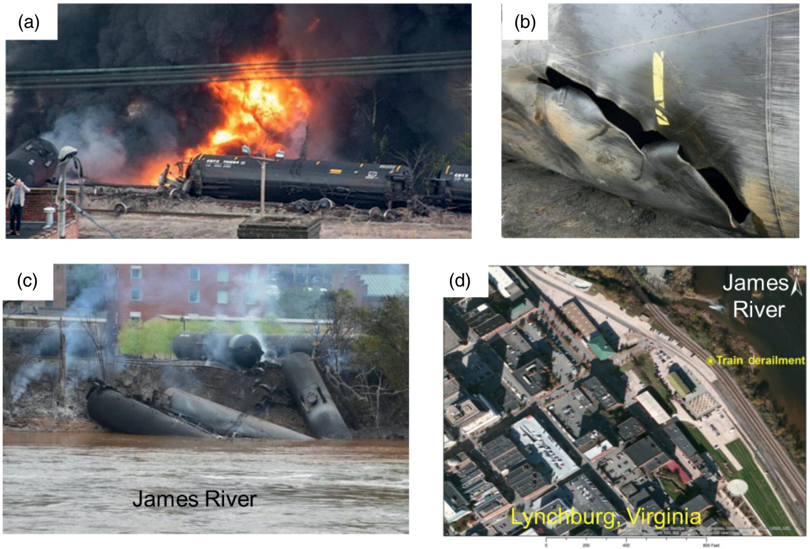
Figure 13.10 Lynchburg, Virginia, railway spill in April 2014: (a) explosion, (b) tear in shell of the tank car, (c) smoldering tank cars in James River, and (d) derailment site
(Photos: NTSB (2017)).
Table 13.25 Description and costs for railway spills.
| Railway spills | Description | Estimated cleanup costs ($) | Cost per gallon spilled |
| Lynchburg, Virginia: 30 April 2014 No injuries |
Major rail or pipeline incidents will cost millions of dollars or more to assess and cleanup. In the CSX spill on 30 April 2014 in Lynchburg, Virginia, 17 tank cars carrying Bakken crude oil derailed out of 105 tank cars. Three of the tank cars were partially submerged in the James River. One of the tank cars was breached and released about 29 868 gal (113 m3) of crude oil into the James River. Some of the oil caught fire | 8.9 million | 29 868 gal = $298/gal |
| Mosier, Oregon: 3 June 2016 No injuries |
A Union Pacific oil train derailment on 3 June 2016 in the Columbia River Gorge near Mosier, Oregon. An estimated 47 000 gal (178 m3) of Bakken crude oil leaked | 8 900 000 | 47 000 gal = $189/gal spilled |
| Mount Carbon, West Virginia: 16 February 2015 No injuries |
A CSX unit train hauling Bakken crude oil from North Dakota to Yorktown, Virginia, derailed on 16 February 2015 near the small town of Mount Carbon along the Kanawha River in Fayette County, West Virginia. Twenty‐seven of the 109 tanker cars derailed, and 19 of the tanker cars caught fire, spilling crude oil into the river. About 378 000 gal (1 431 m3) of crude oil was released. The costs do not include lawsuits or regulatory fines | 23 000 000 | 378 000 gal = $61/gal spilled |
| Casselton, North Dakota: 30 December 2013 No injuries |
Thirteen cars in a westbound BNSF Railway (BNSF) grain train derailed near Casselton, North Dakota/fouling an adjacent main track on 30 December 2013. During the derailment, an eastbound BNSF Bakken crude oil unit train with 106 cars was traveling on the adjacent track. Eighteen of the 21 derailed tank cars ruptured, spilling an estimated 400 000 gal (1 514 m3) of Bakken crude oil | 8 000 000 | 400 000 gal = $20/gal spilled |
| Aliceville, Alabama: 8 November 2013 No injuries |
A 90‐car Bakken crude oil train operated by Alabama & Gulf Coast Railway derailed in a rural Alabama near the town of Aliceville on 8 November 2013. Cleanup costs were estimated at $3.9 million. The spill was characterized as 748 000 gal (2 831 m3) of oil in the derailed tanker cars; 208 952 gal (791 m3) was transferred from the damaged cars, and 19 642 gal (74 m3) of oil was recovered from the water surface. 8000 tons (7257 t) of soil was excavated, and 539 751 gal (2 043 m3) of Bakken crude oil was discharged into the environment | 3 900 000 | 539 751 gal = $7/gal spilled |
13.7.5 Pipeline Leaks
A Bakken crude oil spill was noted by the US EPA On‐Scene Coordinator report (US EPA 2015) for the 17 January 2015 incident in the Yellowstone River pipeline crossing area. The pipeline operator, Bridger Pipeline, observed abnormal pressure readings prior to the release. The pipeline was shut down. A release was discovered four hours later in the river. Estimates for the release from the 12 in (30.5 cm) diameter pipeline range from 300 barrels (12 600 gal; 47.6 m3) to 1200 barrels (50 400 gal; 190.8 m3).
A pipeline leak which occurred on 30 September 2013 released 20 600 barrels (865 200 gal; 3 275.1 m3) of Bakken crude oil in a farm field in Mountrail County, North Dakota, about 900 ft by 1500 ft (274 m × 457 m), with a distance to the nearest surface water estimated at 0.5 mile (0.8 km). Tesoro Logistics Pipeline was the operator of the pipeline and responsible party (NDDH 2013). Lateral extent of contamination was noted as 7.3 acres or 3.0 ha (ha). Field burning occurred on 3 acres (1.2 ha). Monitoring wells were installed.
13.8 Summary
Unconventional oil and gas drilling, completions, and production operations are being performed worldwide on an unprecedented scale. Accidents, leaks and spills, and other environmental impacts are inevitable for the industrial process of extracting, transporting, and refining unconventionally produced oil and gas, even under the best of circumstances. Three aspects of the industrial scale of these possible impacts on water resources can be noted:
- Given the large number of unconventional oil and gas wells, even if only 1% of all wells experience an incident, such as a regulatory violation or reportable spill or leak of contaminants, the number of incidents is large. For example, if 1 million wells are drilled, 1% is 10 000 incidents. Of the number of total incidents, only a small number of incidents or regulatory violations are likely to create environmental or health‐related impacts, but localized impacts to groundwater or other resources have occurred and will continue to occur.
- A generally low regional accident or spill rate per unconventional well drilled does not provide relief for the damaged party impacted by a rare well site‐related incident.
- Rare but large railcar, pipeline, tanker truck, barge, or ship accident spills related to unconventional oil and gas transportation do occur and can have lasting and profound impacts on surface water and groundwater resources and ecosystems.
13.9 Exercises
Table for Exercises 13.1–13.3
| Remedial options | $2017 | Duration of project | Likelihood of success (%) |
| Phytoremediation | $15/cubic yard | 10 years+ | 35 |
| Chemical oxidation | $50/cubic yard | 1–2 years | 60 |
| Enhanced bioremediation | $75/cubic yard | 2–5 years | 45 |
| Thermal treatment | $125/cubic yard | 6 months | 75 |
| Over‐excavation and import of clean fill | $175/cubic yard | 3 months | 95 |
- 13.1 As a consultant, you were called to treat 5000 cubic yards (3823 m3) of contaminated soil. The soil has crude oil mixed with drilling muds. The likelihood of success was based on experience of the contractor and a series of feasibility studies in the laboratory. If your client is interested in the Green and Sustainable Remediation approach, which technology would you use?
- 13.2 Please provide justifications for your answer in Exercise 13.1.
- 13.3 If your client wants to redevelop the property with a K–12 school, which method would you likely select?
- 13.4 Please provide justifications for your answer in Exercise 13.3.
- 13.5 You work for a private lender who is considering funding a multi‐well unconventional oil project in the Williston Basin in eastern Montana. The chances of finding crude oil in economic quantities are high (85%), and the loan will be set at an attractive interest rate. Each well is estimated to cost $6 million each and generate 20 times that amount in gross profit over 30 years. Assuming you are looking at an application for a $60 million loan, explain at least two financial risk strategies in detail to the owner of the private lending company in order to make the loan.
- 13.6 One hundred gallons of waste hydraulic oil was spilled on the drill pad when a backhoe hit two 55 gal drums of waste oil. First responders collected 40 gal (151 l) of fluid and 5 cubic yards of impacted soil for disposal. Due to heavy rains at the time and the natural topography, the remaining waste oil settled in a low area that is designated as a protected wetland. As the environmental regulator for largely rural Salem Township in Westmoreland County in southwestern Pennsylvania, you have to decide whether the 10 discrete soil samples collected from 0.5 to 1.0 ft (0.15–0.3 m) below ground surface showing 50–100 mg kg−1 diesel residual concentrations in soil are worth the impacts to the wetlands to remove the impacted soil.
- 13.7 Please provide justifications for your answer in Exercise 13.4.
- 13.8 As a long‐time real estate agent in Greene County in southwest Pennsylvania, you represent a farmer who wants to sell a 160‐acre (65‐ha) farm on well water. The seller also owns the mineral rights, but no coal mines or gas wells exist on the property. Marcellus Shale wells are currently producing natural gas in the next valley. Assuming the buyer buys the farm with the mineral rights, what disclosures and notifications should be given by the seller to the buyer? What environmental concerns should be addressed?
- 13.9 As the real estate agent, make a chart of disruptions, nuisance issues, timing of well drilling, and possible benefits that a buyer could reasonably expect if 2 Marcellus Shale gas wells are to be drilled 2000 ft (610 m) away from the farmhouse. The buyer should be informed that when the operator moves into the valley to produce gas, the bonus payments for a 160‐acre (65‐ha) farm are $3200 per acre and the gas royalty is 12.5%.
- 13.10 Your uncle owns a farm in Bradford County, Pennsylvania. The operators have contacted him about leasing his land for Marcellus Shale gas production. You were asked to help him consider his first‐year windfall. Assume a signing bonus of $3500 per acre and a production royalty rate of 10% with an average wellhead natural gas price of $3.00 per thousand cubic feet per day. How much will the farmer get in one year of production including the signing bonus?

where
- RR = royalty rate (%)
- DP = daily production (Mcf)
- AWP = average wellhead price ($ per Mcf)
- Mcf = thousand cubic feet of natural gas
- MMcf = million cubic feet of natural gas
- AO = acres owned (acres)
- TA = total acres in well production unit (acres)
- ARP = annual royalty payment ($)
Natural gas royalty calculation Rates Royalty rate 10% Average wellhead natural gas price $3.00 per thousand cubic feet (Mcf) Average well production rate (entire production unit) 10 million cubic feet per day Acres (owned by farmer) within the well production unit 500 acres (202 ha) Total number of acres within the well production unit 800 acres (324 ha)
References
- Abramzon, S., Samaras, C., Curtright, A. et al. (2014). Estimating the consumptive use costs of shale natural gas extraction on Pennsylvania roadways. Journal of Infrastructure Systems 20, 12 p.
- Bell, R.B. and Bell, M.P. (2017). Hydraulic fracturing and real estate issues. The Appraisal Journal, The Appraisal Institute, Winter 85: 9–17.
- Brewer, R. (2018). Environmental Investigation and Development of “Brownfield Sites” in Hawaii, Department of Health Hazard Evaluation and Emergency Response, Brownfield Kauai County Development and Land Reuse Redevelopment Workshop 2018, Kauai, Hawaii, US, 10 July, 6 p.
- California Department of Water Resources (DWR) (1981). Water Well Standards: State of California, Bulletin 74–81. Department of Water Resources, Sacramento, CA, 55 p. https://water.ca.gov/LegacyFiles/pubs/groundwater/water_well_standards__bulletin_74‐81_/ca_well_standards_bulletin74‐81_1981.pdf (accessed 22 October 2018).
- Christie, S. (2010). Protecting our roads. Testimony before the Pennsylvania House Transportation Committee. 10 June.
- CostHelper Home and Garden (CostHelper) (2017). Well drilling cost, how much does well drilling cost? Retrieved 20 September 2017; http://home.costhelper.com/well‐drilling.html.
- Department for Toxic Substances Control (2009). Interim advisory for green remediation. California Environmental Protection Agency, December, 40 p.
- Dutzik, T., Ridlington, E., and Rumpler, J. (2012). The Costs of Fracking: The Price Tag of Dirty Drilling's Environmental Damage. Minneapolis, MN: Environment Minnesota Research & Policy Center.
- Elswick, F. (2016). How much does it cost to build a mile of road? Midwest blog, p. 9.; Retrieved 30 September 2017; http://blog.midwestind.com/cost‐of‐building‐road.
- Gunderson, D. (2012). Oil Boom and the North Dakota Economy. Minnesota Public Radio. 4 January; Retrieved 30 September 2017; http://www.commerce.nd.gov/news/detail.asp?newsID=1063.
- Heinberg, R. (2013). Snake Oil: Chapter 5 – the economics of fracking: who benefits? Resilience. 23 October; Retrieved 30 September 2017; http://www.resilience.org/stories/2013‐10‐23/snake‐oilchapter‐5‐the‐economics‐of‐fracking‐who‐benefits#.
- HIDOH (2017). Evaluation of Environmental Hazards at Sites with Contaminated Soil and Groundwater – Hawaii Edition (Fall 2017): Hawai'i Department of Health, Office of Hazard Evaluation and Emergency Response. Retrieved 23 October 2017; http://eha‐web.doh.hawaii.gov/eha‐cma/Leaders/HEER/EALs.
- Interstate Technology & Regulatory Council (ITRC) (2012). Incremental Sampling Methodology. ISM‐1. Washington, DC: Interstate Technology & Regulatory Council, Incremental Sampling Methodology Team www.itrcweb.org.
- Integra Realty Resources (IRR) (2010). Flower Mound well site impact study, Dallas, TX, p. 108.
- Interagency Land Acquisition Conference (ILAC) (2016). Uniform Appraisal Standards for Federal Land Acquisitions, p. 262.
- Kelso, M. (2015). 1.7 Million Wells in the U.S. – A 2015 Update, Updated National Well Data, FracTracker Alliance, 3 August, 8 p.; Retrieved 29 September 2017; https://www.fractracker.org/2015/08/1‐7‐million‐wells.
- Ladlee, J.R. (2017). Natural Gas Production Decline Curve and Royalty Estimation, Penn State Extension, 8 August, 6 p.; Retrieved 21 October 2017; https://extension.psu.edu/natural‐gas‐production‐decline‐curve‐and‐royalty‐estimation.
- Moss, K. (2008). Potential Development of the Natural Gas Resources in the Marcellus Shale: New York, Pennsylvania, West Virginia and Ohio. Denver, CO: National Park Service, US Department of the Interior, Geologic Resources Division.
- Muehlenbachs, L., Spiller, E., and Timmins, C., 2015a, The Housing Market Impacts of Shale Gas Development, 2015. American Economic Review, Vol. 105, No. 12, Dec., pp. 3633–3659.
- Muehlenbachs, L., Spiller, E., Steck, A., and Timmins, C. (2015b). The Impact of the Fracking eBoom on Rents in Pennsylvania, 15 February, 31 p.; Duke University, Durham, NC. http://public.econ.duke.edu/~timmins/fracking_rents.pdf (accessed 22 October 2018).
- National Groundwater Association (NGWA) (2016). 2016 NGWA Contractors Survey. Columbus, OH: National Groundwater Association, 2 p.
- National Transportation Safety Board (NTSB) (2017). Railroad Accident Brief, CSXT Petroleum Crude Oil Train Derailment and Hazardous Materials Release, DCA14FR008, 30 April 2014, Lynchburg, Virginia, NTSB/RAB‐16/01, report reissued on 3 April2017, 13 p.
- New York State (2011). Supplemental Generic Environmental Impact Statement, (SGEIS). Department of Environmental Conservation, August, 1448 p.
- North Dakota Department of Health (NDDH) (2013). General Environmental Incident Summary, Incident 2056, Environmental Health Section. Report #EIR2056, Incident Date: 9/29/13, Report by Eric Haugstad, Tesoro Logistics Pipeline, 13 p.; Retrieved 18 November 2017; http://www.ndhealth.gov/EHS/FOIA/Spills/Summary_Reports/EIR2056_Summary_Report.pdf
- Pennsylvania Department of Environmental Protection (PDEP) (2017). Environmental Good Samaritan Act, Updated 10/18/2017, 2 p.; Retrieved 27 October 2017; http://files.dep.state.pa.us/OilGas/BOGM/BOGMPortalFiles/OilGasReports/2017/GOOD_SAMARITAN/Good_Sam_Project_List.pdf.
- Podulka, S.G. and Podulka, W.J. (2010). Comments on the Science Advisory Board's 5/19/2010 Draft Committee Report on the US EPA's Research Scoping Document Related to Hydraulic Fracturing Report.
- Ritzel, B. (2015). Critical Assessment of the Literature Regarding the Public Costs of Roadway Damage Due to Fracking, Southern Illinois University, Carbondale, IL, Research Papers, Graduate School, 71 p.
- Rogers, D.L. (2013). Externalities of shales: road damage. Energy Policy Forum. 1 April.
- San Francisco Regional Water Quality Control Board (SFRWQCB) (2016). User's Guide: Derivation and Applications of Environmental Screening Levels (ESLs). Interim Final 2016, 237 p.
- Throupe, R., Simons, R., and Mao, X. (2013). A review of hydro “Fracking” and its potential effects on real estate. Journal of Real Estate Literature 21 (2): 205–232.
- United States Energy Information Administration (US EIA) (2016). Hydraulically fractured wells provide two‐thirds of U.S. natural gas, 5 May, 2 pages; Retrieved 29 September 2017; https://www.eia.gov/todayinenergy/detail.php?id=26112.
- U.S. Environmental Protection Agency (US EPA) (2015). Bridger Pipeline Release, Glendive, Montana, Region VIII, Paul Peronard, On‐Scene Coordinator; Retrieved 18 November 2017; https://response.epa.gov/site/site_profile.aspx?site_id=9708.
- U.S. Environmental Protection Agency (US EPA) (2017). Software Packages and Online Tools, Clu‐In, Contaminated Site Clean‐Up Information; Retrieved 15 October 2017; https://clu‐in.org/software.
- White, N.E. (2013). A tale of two shale plays. 2012 SRSA Fellows Address. The Review of Regional Studies 42 (2): 107–119.
Suggested Reading
- Department of Water Resources (DWR) (1990). Water Well Standards: State of California, Bulletin 74–90 (Supplement to Bulletin 74–81). Sacramento, CA, 93 p. https://water.ca.gov/LegacyFiles/pubs/groundwater/water_well_standards__bulletin_74‐90_/ca_well_standards_bulletin74‐90_1991.pdf: Department of Water Resources accessed 22 October 2018.
- Santa Clara Valley Water District (SCVWD) (2017). A Guide for the Private Well Owner, PUB 605.1; May, Version 18. San Jose, CA: SCVWD, 20 p.
- Underground Storage Tank Cleanup Fund (USTCF) (2014). Cost Guidelines Update January 1, 2014, State Water Resources Control Board (SWRCB), Sacramento, California, 47 p.
- U.S. Army Center for Excellence (USACE) (2012). Conceptual Site Models for Ordnance and Explosives (OE) and Hazardous, Toxic, and Radioactive Waste (HTRW) Projects. EM 200–1‐12. https://www.itrcweb.org/ism‐1/references/EM_200‐1‐12.pdf.