9
Land Use Resources and Socioeconomics
9.1 Introduction
Of all the categories of possible impacts, land use resources and socioeconomics may be the broadest category with impacts that are most noticeable to communities living near well sites and mine sites. These social issues include community quality‐of‐life issues, as well as environmental justice, health and safety for the community and workers, worker training, historic and cultural resource protection, and land use planning. The Shale Gas Roundtable (Gourley et al. 2013) report summarized two main land use concerns and one main land use opportunity in unconventional oil and gas‐producing areas:
- Minimize the acute and cumulative impacts of oil and gas operations on the environment, public health, and local communities.
- Minimize the surface disturbance from oil and gas operations, and optimize the efficiency of resource recovery and transport to market.
- Enhance the use of unconventional oil and gas, and support opportunities for regional and national economic growth based on the full oil and natural gas value chain.
Land use resources and socioeconomics are impacted to varying degrees by all seven phases of the unconventional oil and gas exploration–production life cycle:
- Phase 1 Prospect generation (geochemistry studies and geophysical surveys).
- Phase 2 Planning (lease acquisition and site preparation).
- Phase 3 Drilling.
- Phase 4 Well completion and hydraulic fracture stimulation.
- Phase 5 Fluid recovery and waste management.
- Phase 6 Oil and gas production.
- Phase 7 Well abandonment and site restoration.
Reviewing the seven phases shows that the most intense impacts such as the local generation of dust, noise, odor, light pollution, and heavy traffic occur in the site preparation, drilling, and development phases: phase 2 (planning – site preparation) through phase 5 (fluid recovery and waste management).
Once the first part of phase 6 (oil and gas production) is completed and the pipelines, storage tanks, and other facilities are in place, the routine operations and maintenance of the field production generally require less intense on‐site activities. Most of the regular production phase includes monitoring, inspection, and repair, but production typically does not have the short‐duration, high‐intensity impacts (such as elevated noise and increased traffic), unless there are specific field projects, such as a well workover.
The main land use and socioeconomic impacts from phase 2 through 5 include:
- Community concerns and land use planning.
- Cultural resource protection.
- Environmental justice.
- Historic resource protection.
- Health and safety – community.
- Health and safety – workers.
- Land disturbance.
- Light pollution.
- Noise.
- Odor.
- Social challenges and issues.
- Transportation and traffic.
- Visual aesthetics.
- Worker training and education.
9.2 Community Concerns and Land Use Planning
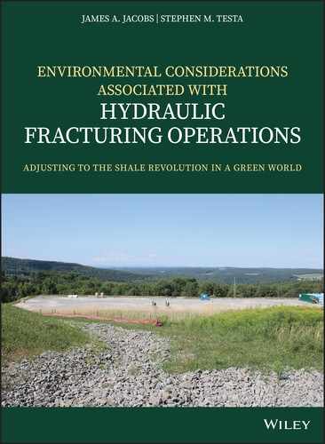
The development of unconventional oil and gas resources changes the overall character of a rural landscape into an industrial setting, but the level of intense 24/7 activity is temporary and only occurs during active operations (Figure 9.1) of phase 2 through the start of phase 6. After the well installation and hydraulic fracturing stimulation and flowback activity ceases and the development starts, the subsequent oil and gas production involves limited activity (Figures 9.2 and 9.3).

Figure 9.1 Active but temporary hydraulic fracturing process at a well in the Marcellus Formation, Pennsylvania, USGS (2017).
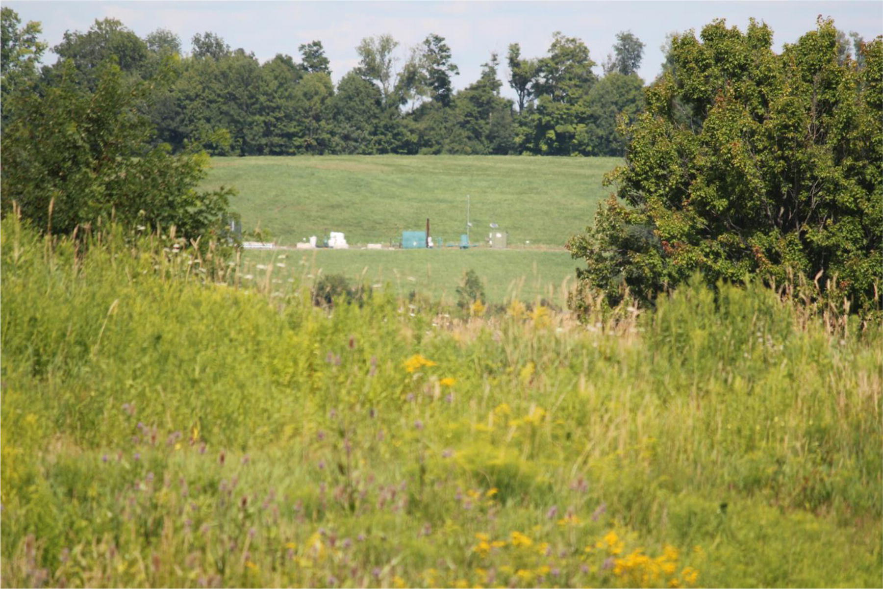
Figure 9.2 Producing gas well in Marcellus Formation, near Dimock, Pennsylvania.
Photo taken from road. Source: Image James A. Jacobs.

Figure 9.3 Unconventional gas production in northeast Pennsylvania. No odors, dust, noise, or erosion were observed.
Source: Image from James A. Jacobs.
9.2.1 Community Issues
Land use and community issues can be addressed in community meetings and public discussions to reduce tension. Some quality‐of‐life issues can be addressed with institutional controls. Institutional controls are administrative or legal controls that prevent or minimize unacceptable human, environmental, or wildlife exposure to hazardous conditions such as contaminants in the air, water, or soil. Institutional controls can also prevent or limit exposure or land use for the purposes of protection. There are four categories of institutional controls for land use planning (ITRC 2008):
- Government controls
- Proprietary controls
- Enforcement and
- Informational devices (see below)
| Institutional controls | Example | Purpose |
| Government controls | Existing ordinances, zoning, building, development, rules, environmental restrictions | Limits or defines the terms of land or resource use |
| Proprietary controls | Deed restrictions, easements, excavation or drilling prohibitions | Controls property activity |
| Enforcement | Permits, administrative orders, and enforcement agreements | Restrict future land use / defines use and consequences of not following rules |
| Informational devices | Deed notices, state registries, public advisories | Notify the public of activity, contamination or other impacts on a property. Sometimes agency websites provide the information. (Example: geotracker.waterboards.ca.gov) |
Governmental agencies can use all four institutional controls to address community issues with unconventional oil and gas development. Existing land use zoning and community plans may be in conflict with the new industrial processes that accompany unconventional oil and gas development. Some community members may suggest that existing lands with agricultural, grazing, mineral extraction, tourism, or recreational uses may not be consistent with the new intended shared use. Specific tracts of lands nearby proposed oil and gas development may have special meaning in the community for educational, religious, or scientific reasons.
9.2.2 Best Management Approach
Implementation of best management practices (BMPs) (Eshleman and Elmore 2013; Gourley et al. 2013) can establish community cooperation through setting operator commitments and goals. Following BMPs can serve to reduce regulatory violations and potential environmental impacts. BMPs in 8 critical areas follow:
1) Field Performance
- Provide rigorous training to all workers.
- Demand excellence from employees.
- Require subcontractors and subvendors to meet high standards and BMPs.
- Strive for overall excellence in project performance.
- Be proactive with regulatory agencies and community leaders.
2) Operator Interactions with Community
- Provide complete transparency with regard to community decisions.
- Allow the public to participate in meetings.
- Secure community consent.
- Hire locally.
- Provide safety and skills training to workers.
3) Environmental Background Studies
- Perform detailed background baseline water sampling of surface water and nearby water wells.
- Document the presence and condition of historic wells.
- Verify water issues prior to drilling.
4) Community Concerns
- Accommodate the rapid influx of workers into rural areas.
- Provide updated skill and safety training so local workers are hired.
- Provide housing for local citizens and new workers.
- Provide and pay for a higher level of public services (police, fire, school, library, etc.) to address changes in the community.
- Maintain or upgrade the condition of local roads and community assets.
- Address public health impacts affecting hospitals, emergency rooms, and health providers.
- Mitigate noise, light, traffic, and other nuisance issues.
- Address tensions between the surface rights owner and the mineral rights owner.
5) Economic Opportunities
- Address the boom‐and‐bust natural resource extraction cycles and their impacts on communities.
- Convert vehicles and other engines to run on natural gas.
- Actively attract new industries and business opportunities focused on low energy costs.
- Create new jobs in the community and encourage local small businesses.
6) Damage and Risk Control
- Create and follow a BMP materials‐ use plan
- Disclose related fines, penalties, and litigation.
- Minimize and disclose air emissions.
- Manage risks transparently and company‐wide at the board level.
- Minimize spillage of hazardous materials by keeping water and fluids in tanks, gas cylinders in flammable storage cabinets, and solids in locked sheds or secured cabinets.
- Inspect hazardous materials regularly, and maintain safety data sheets (SDS) binders.
- Maintain several hazardous materials spill response kits on‐site and train workers.
7) Environmental Disclosure and Recycling
- Reduce and disclose all toxic chemicals used on‐site, including the special chemical additives.
- Use green completions, where possible.
- Avoid natural gas flaring and provide waste gas to local businesses instead.
- Recycle water and fluids.
- Remove wastes from site promptly.
8) Environmental Protection
- Train workers and provide equipment to contain hazardous materials and wastes.
- Prevent site contamination from solid waste and sludge residuals.
- Prevent site contamination from liquid wastes by containment.
- Protect water quality by regular inspections as well as maintaining a groundwater and surface water monitoring program to identify problems promptly.
- Minimize the surface footprint of the well pad and access roads.
- Verify well integrity and fix when detected.
9.2.3 Setbacks
Setbacks may provide the best level of local control to reduce industrial activity exposures of elevated noise, odor, and dust. Setbacks can also provide relief from visual impacts. A minimum of 1000 ft (305 m) between wellheads and compressor stations to any occupied building will reduce noise impacts. Setbacks designed for use in the state of Maryland provide an example of a regulatory standard for setbacks (Table 9.1).
Table 9.1 Example of setbacks.
Source: From Eshleman and Elmore (2013).
| Receptor | Source of exposure or disturbance | Distance between source and receptor | |
| (ft) | (m) | ||
| Aquatic habitat (defined as all streams, rivers, seeps, springs, wetlands, lakes, ponds, reservoirs, and floodplains) | Edge of drill pad disturbance | 300 | 91 |
| Special conservation areas (e.g. irreplaceable natural areas, wildlands) | Edge of drill pad disturbance | 600 | 183 |
| All cultural and historical sites, state and federal parks, trails, wildlife management areas, scenic and wild rivers, and scenic byways | Edge of drill pad disturbance | 300 | 91 |
| Mapped limestone outcrops or known caves | Borehole | 1000 | 305 |
| Mapped underground coal mines | Borehole | 1000 | 305 |
| Historic gas wells | Any portion of the borehole, including laterals | 1320 | 402 |
| Any occupied building | Compressor stations | 1000 | 305 |
| Any occupied building | Borehole | 1000 | 305 |
| Private groundwater wells | Borehole | 500 | 152 |
| Public groundwater wells or surface water intakes | Borehole | 2000 | 610 |
9.2.4 Cultural Resource Protection and Historic Resource Protection
Impacts from oil and gas operations include the potential for the discovery and destruction of significant cultural resources in areas undergoing surface disturbance. Examples would include the geophysical survey and more importantly during well pad or access road construction or during sand and gravel mining. Unauthorized removal or destruction of cultural artifacts or vandalism as a result of new access roads or discovery during subsurface excavation reduces the educational, scientific, and recreational opportunities for further research and interpretive display of these features or articles. In areas where the cultural resources are associated with the shape and topographic features of the landscape, cultural resources such as tribal sacred landscapes may be harmed. If possible, care should be taken to avoid historic artifacts such as the footprint of former villages, historic trails, or petroglyphs. Increased erosion and additional vibration caused by geophysical surveys, drilling activities, or increased heavy traffic may dislodge or uncover buried artifacts (TEEIC 2017).
Some of the same environmental conditions that are optimal for oil and gas operations, such as easy access to abundant surface water and a location with transportation access, may have been similar for inhabitants in the same area for hundreds or thousands of years. A large percent of archaeological sites which were identified within the entire Red River alluvial valley in northeast Texas were preferentially located in areas surrounding prehistoric oxbow lakes on the floodplain; this compared with a low percent of sites located in elevated fluvial terraces or in bedrock locations higher up the slopes (Jacobs 1980). Not surprisingly, the same prehistoric oxbow lakes today would be attractive as a potential source for water resources for unconventional oil and gas operations. Prior to field work, appropriate field surveys for cultural sites and historic artifacts should be performed in areas to be disturbed, especially in areas slated for pipeline trenching. Awareness training of workers should also be performed due to the potential of encountering or disturbing cultural sites or historic artifacts. Preparing protocol for stop work and scope change insures that projects can efficiently proceed when cultural sites are encountered.
9.3 Environmental Justice
If significant impacts occur during the exploration and production of the unconventional oil and gas resources that disproportionally affect minority, low‐income, or tribal populations, environmental justice issues may be present (TEEIC 2017). On the upside, job opportunities, training, and the development of long‐term growth may provide financial stability to economically distressed regions. Project revenues may also encourage increased tourism. Drawbacks include the increase of noise, odor, dust, visual impacts, habitat fragmentation, and destruction.
9.4 Land Disturbance
Erosion and sedimentation are among the most significant impacts of land disturbance and habitat destruction that occur during the building of drilling pads and the construction of access roads. In areas with heavy rain, rill and deep erosion can occur.
Land disturbance during unconventional oil and gas exploration and development can impact a variety of ecosystem processes:
- Abiotic ecosystem processes.
- Acid rock drainage.
- Native plant communities.
- Interaction between plants and animals.
- Variations in native genetic diversity.
9.4.1 Abiotic Ecosystem Processes
Abiotic ecosystem changes are caused by a variety of geologic processes that can dramatically change habitat and land conditions. Abiotic changes can include stormwater erosion, rainwater infiltration, microdrainage changes, changes in fire potential, and changes in nutrient cycling.
9.4.2 Acid Rock Drainage
Acid rock drainage is common in newly developed areas where pyrite‐rich rocks are exposed on the surface to oxygen and water. Pyrite, the most common iron sulfide (FeS2), is also known as “fool’s gold.” The reduced sulfide mineral pyrite is often associated with valuable resources like coal, gold, copper, and silver deposits. The oxidation of pyrite and the release of toxic metals can occur in any area undergoing land disturbance containing pyrite‐rich rocks.
Catalyzed by a community of microorganisms with iron‐ and sulfur‐oxidizing bacteria, the biogeochemical process creates acid rock drainage by generating sulfuric acid (H2SO4). Once the drainage pH is lowered to 2 or 3 by the sulfuric acid, soluble metals such as iron, arsenic, cadmium, copper, lead, nickel, and zinc are dissolved into the acidic waters. Precipitation of the dissolved metals occurs downstream. Fish kills have been documented in streams and rivers impacted by significant acid rock drainage (Jacobs et al. 2014, 2016).
The presence of acidophilic microbes reflects a community that thrives when conditions are acidic, but pyrite oxidation and acid generation occur with microbes in circumneutral pH environments (Konhauser 2007). As the drainage becomes more acidic, the microbial community evolves, until only acidophiles, microbes capable of thriving in lower pH (2 or 3) environments, remain. The sulfur‐ and iron‐oxidizing microbial community includes primarily bacteria and archaea and, to a minor degree, fungi, yeasts, protozoans, microalgae, and rotifers (Baker and Banfield 2003; Robbins et al. 2000).
As land disturbance for unconventional oil and gas exploration and development starts, if pyrite‐rich rocks are exposed, natural acid drainage could be produced. The first phase in pyrite oxidation process is shown below:
The dominant microbial pathway for pyrite dissolution involves oxidation of ferrous iron [Fe(II)] by oxygen:
This is followed by reduction of ferric iron [Fe(III)] by disulfide in pyrite:

9.4.3 Acid Rock Drainage Mitigation
Acid rock drainage mitigation requires the geologic assessment of whether zones of pyrite‐rich rocks occur near the surface that will be disturbed during the unconventional exploration or development process. If nearby coal or mineral mines produce acid mine drainage, pyrite‐rich rock may occur near the surface. Covering pyrite‐rich rock layers with soil and planting erosion control vegetation can reduce the potential for acidic drainage. Acid neutralization using lime or hydroxides is an ongoing operational chemical treatment method used once the acidic drainage starts. Once the acid drainage starts, stopping the biogeochemical process is difficult and costly.
9.4.4 Native Plant Communities
Land disturbance on an ecosystem will impact the native plant community composition, structure, and interactions with other plants, microorganisms, fungi, and animals. Land disturbance also impacts the interactions of higher trophic levels, including vertebrates and invertebrates, and the genetic integrity of native species. Rapid human‐caused land disturbance can generate hybrid habitats of many types, resulting in hybrid plants. Hybridization may drive rare taxa to extinction through genetic swamping, where the rare form is replaced by more robust hybrids, or by demographic swamping, where population growth rates are reduced due to the wasteful production of maladaptive hybrid traits (Todesco et al. 2016).
Endangered, rare, and threatened native species of animals as well as plants, as varied as trees, shrubs, vines, flowers, and grasses, are especially at risk during the land disturbance phase. Native plants and animals, having developed in a specific ecosystem, often occur in such small numbers that land disturbance will make them particularly vulnerable to habitat destruction and competition from invasive species.
Invasive plants are highly adaptable generalists and are noted for their ability to grow and spread aggressively. Invasive plant species have several similar characteristics:
- Reproduce rapidly by roots, seeds, shoots, or all three.
- Mature quickly.
- Difficult to remove once established.
- Form a monoculture by monopolizing the ecosystem.
- Outcompete native plants for resources.
- Tend to be more robust and hardy in drought or other difficult weather conditions.
- If spread by seed, produce numerous seeds that disperse and sprout easily.
9.4.5 Invasive Plants
Examples of invasive plants in the United States include kudzu (Pueraria montana var. lobata), purple loosestrife (Lythrum salicaria), Japanese honeysuckle (Lonicera japonica), Japanese barberry (Berberis thunbergii), English ivy (Hedera helix), garlic mustard (Alliaria petiolata), Uruguayan pampas grass (Cortaderia selloana), Scotch broom (Cytisus scoparius), yellow starthistle (Centaurea solstitialis), bull thistle (Cirsium vulgare), and blue gum eucalyptus (Eucalyptus globulus). Invasive species can replace native plants and degrade habitat for native insects, birds, and animals.
9.4.6 Land Disturbance Mitigation
The best way to prevent invasive plant species is to minimize the impact areas and to seed the disturbed areas with native plant seeds soon after the land disturbance occurs. Regular site inspections and photo documentation are recommended to verify that invasive species do not get established. Dust control and stormwater pollution prevention plans (SWPPPs) can be designed to minimize erosion and stormwater impacts during land disturbance activities.
Burning does not provide long‐term control, as invasive plants resprout shortly thereafter. Infestations sometimes can be averted by overseeding open disturbed sites with native seeds to prevent establishment of invasive plant seedlings. Pulling or hand grubbing invasive plant seedlings is not only labor‐intensive but also an effective method of physical control. Chemical control and burning are not recommended for invasive plant species removal as other native species may be harmed.
9.5 Light Pollution
Extraneous light pollution has become a significant issue at numerous unconventional oil and gas operations. The two sources of light pollution at drill sites include:
- Artificial lighting
- Flaring of unwanted gas
Artificial lighting is used to illuminate the site or access roads from the drill pad to the main transportation routes. Electric lights can be focused on the ground and encased in shrouds to eliminate light pollution.
Lighting and flaring mitigation measures can reduce light pollution (Eshleman and Elmore 2013). One way to reduce lighting impacts on migrating birds, is to use green light and ultraviolet (UV) filters, which were found to be less disorienting than red or blue light (Poot et al. 2008; Wiltschko et al. 1993).
9.5.1 Lighting Mitigation Measures
BMPs to limit light pollution and reduce glare and shadows include:
- Directing light sources downward.
- Limiting the duration of lighting.
- Focusing lights low to the ground.
- Limiting the lighting column height to less than about 26 ft (8 m).
- Reducing lighting to illuminate only required areas.
- Lowering the intensity of the lighting, as safety will permit.
- Using light shrouds, caps, and diffusing fabrics to minimize light diffusion.
- Using the most energy‐efficient lights:
- Use low‐pressure sodium lamps instead of high‐pressure mercury lamps.
- Use UV filters, where possible.
- Use green light rather than red or blue light (less disorienting to migrating birds).
- Using light activation sensors to provide lighting only when needed.
9.5.2 Flaring Mitigation Measures
When pipelines are not available to transport the natural gas to market, flaring addresses the issue of destroying unwanted natural gas that is coproduced with oil (Figure 9.4). Flares burn the natural gas in a controlled and safe manner; however, the waste of energy is not a sustainable or environmentally appropriate long‐term practice. Light pollution from flaring of natural gas is so bright in the Williston Basin that the light can be seen from extra terrestrial satellites (Figure 9.5).

Figure 9.4 Flares of natural gas from the Bakken Formation in western North Dakota produce both noise and light pollution.
Source: Image from North Dakota Department of Health.

Figure 9.5 Flares of natural gas from the Bakken Formation in western North Dakota are visible from space. Inset is the night satellite view of the United States and Canada.
Source: Image from NASA.
BMPs for natural gas flaring include the following:
- Flaring as a practice should be eliminated or significantly minimized.
- Reuse the flare gas in an incinerator, which conceals the flame.
- Reuse the wasted natural gas and pipe for local needs, such as heating greenhouses or generating electricity.
- Collect the coproduced natural gas.
- If possible, place flare stacks in less visible locations.
9.6 Noise
From an environmental context, noise is unwanted sound. A variety of regulatory agencies generally define nuisance noise as loud, jarring, discordant, and disagreeable sounds. Sound propagates as a wave of positive pressure disturbances (called compressions) interspersed with negative pressure disturbances (called rarefactions) (Figure 9.6). The wavelength (λ) is the distance a sound wave travels during one sound pressure cycle (Figure 9.7).
Figure 9.6 Concept areas of compression, rarefaction and of a sound wave (OSHA 2013).

Figure 9.7 General concept of wavelength (OSHA 2013).
According to OSHA, noise, or unwanted sound, is one of the most common occupational hazards in American workplaces. The National Institute for Occupational Safety and Health (NIOSH) estimates that 30 million workers in the United States are exposed to hazardous noise. Exposure to high levels of noise may cause hearing loss, create physical and psychological stress, reduce productivity, interfere with communication, and contribute to accidents and injuries by making it difficult to hear warning signals. Besides workers, noise from unconventional oil and gas operations can impact nearby residents and communities.
Frequency (f) is the total number of vibrations or sound pressure cycles that occur per second. Frequency is measured in hertz (Hz). One hertz is equal to one cycle per second. Sound frequency is perceived by the human ear as pitch, which is the degree of highness or lowness of a tone. The frequency range sensed by the human ear varies considerably among individuals. A young person with normal hearing can hear frequencies between ~20 and 20 000 Hz. As one ages, the highest detectable frequency tends to decrease. Human speech frequencies generally range from 500 to 4000 Hz (OSHA 2013).
9.6.1 Speed of Sound
The speed at which sound travels (c) is determined primarily by the density and the compressibility of the medium through which it is traveling. The speed of sound is typically measured in feet per second (meters per second). The speed of sound increases as the density of the medium increases and its elasticity decreases. In air, the speed of sound is ~1129 ft s−1 (344 m s−1) at standard temperature and pressure. However, in liquids and solids, the speed of sound is much higher. In water, the speed of sound is about 4921 ft s−1 (1500 m s−1), and in steel, the speed of sound is about 16 404 ft s−1 (5000 m s−1).
The frequency, wavelength, and speed of a sound wave are shown by the equation
where c is the speed of sound in meters or feet per second, f is the frequency in Hz, and λ is the wavelength in feet or meters.
Common background noise levels from numerous sources show the noise range measured in dBA (Table 9.2). The primary sources of noise associated with unconventional oil and gas exploration and production start with the phase I prospect generation tasks. These include the short‐duration, sporadic, but loud blasting noise from the geophysical survey and site preparation activities (Table 9.3).
Table 9.2 Common background noise levels.
| Description | SPL (dBA) |
| Rocket launching from pad | 180 |
| Artillery fire at 500 ft (152 m) | 150 |
| Jet engine taking off | 150 |
| Jet engine at 82 ft (25 m) | 140 |
| Jackhammer, power drill, jet aircraft at 328 ft (100 m) | 130 |
| Pneumatic drills, heavy machine operation, thunder | 120 |
| Pneumatic chipper at 5 ft (1.5 m) | 110 |
| Jointer or planer | 100 |
| Chain saw | 90 |
| Heavy truck traffic, noisy restaurant | 80 |
| Business office, freeway traffic | 70 |
| Typical urban area, conversational speech, air‐conditioning window unit at 25 ft (7.6 m) | 60 |
| Typical suburban area, library | 50 |
| Quiet suburban area at night, bedroom | 40 |
| Rural area at night, secluded woods | 30 |
| Whisper | 20 |
Table 9.3 Description of primary noise sources, examples, and duration.
| Phase | Description | Examples of noise | Duration |
| Phase 1 | Prospect generation (geochemistry studies and geophysical surveys) | Blasting or seismic sources for geophysical survey; seismic trucks, heavy vehicles | Sporadic and short duration |
| Phase 2 | Planning (lease acquisition and site preparation) | Blasting when needed in hilly terrain or with shallow bedrock; bulldozers, graders, excavators and dump trucks for well pad and access road construction, heavy vehicles | Up to 24/7 for several weeks |
| Phase 3 | Drillinga | Drilling rig, pumps, cement grout mixers, generators, loaders and forklifts, heavy vehicles | Up to 24/7 for several months depending on target depth |
| Phase 4 | Well completion and hydraulic fracture stimulation | Proppant and chemical blenders and pumps; loaders and forklifts, heavy vehicles | Up to 24/7 for several weeks |
| Phase 5 | Fluid recovery and waste management | Pumps, separators, heavy vehicles, loaders and forklifts. Noise from flaring of gas | Up to 24/7 for several weeks |
| Phase 6 | Oil and gas production | Pumps, compressors, separators, and heavy vehicles. Noise from flaring of gas | Sporadic and short duration, over several decades. Occasional industrial activities (workovers) or equipment turn‐on (compressors or pumps) |
| Phase 7 | Well abandonment and site restoration | Drilling rig, pumps, generators, and concrete grout mixers for well abandonment. Bulldozers, graders, excavators, and dump trucks for well pad and access road full restoration | Up to 24/7 for several weeks |
aDrilling noise has been measured at 225 dBA at the drill rig (source) and 55 dBA at distances of 1800 ft (549 m) to 3500 ft (1067 m) from the well (TEEIC 2017).
A free field is a region where there are no reflected sound waves between the source and the receptor or measuring device (Figure 9.8). The inverse square law of acoustics shows that each time the distance from the point source is doubled, the sound pressure level (SPL) decreases 6 dB (OSHA 2013). When sound‐reflecting objects such as topographic relief, building walls, or equipment are introduced into the sound field, the wave picture becomes more complicated as sound is reflecting back in other directions and reverberates. Oil and gas field drilling and production tasks generally occur under these more complicated sound reverberation conditions (Figure 9.9).
Figure 9.8 Sound pressure levels (dB) in a free field, distance in meters (OSHA 2013).
Figure 9.9 Sound reverberation showing the original and reflected sound waves (OSHA 2013).
Per figure 9.8, if a point source in a free field produces an SPL of 90 dB at a distance of 3.3 ft (1 m), the sound level is 84 dB at 6.6 ft (2 m) and 78 dB at 13.1 ft (4 m).
Early sound studies of frequency (Hz) plotted against SPL (dB) were performed in 1933 by Harvey Fletcher and Wilden A. Munson. Fletcher and Munson (1933) showed that as the actual loudness of a sound changes (as measured in SPL (dB)), the perceived loudness as interpreted by the average human listener with normal hearing changes at a different rate, depending on the frequency. The Fletcher–Munson curves shows equal loudness contours (Figure 9.10) for the human ear. The nonlinearity of the response of the human ear is represented by the changing contour shapes as the SPL (dB) is increased, especially noted at low frequencies. The lower dashed curve indicates the threshold of human hearing and represents the SPL (dB) necessary to trigger the sensation of hearing in the average human listener. Among healthy individuals, the actual hearing threshold may vary by as much as 10 dB in either direction (OSHA 2013).

Figure 9.10 Equal loudness contours for the human ear (OSHA 2013).
Regarding oil and gas field noise levels, the well installation and development activities include the drilling rig sounds and associated equipment noise while installing the well and performing the hydraulic fracture stimulation and flowback management. Gas flaring does generate continuous combustion noise while flaring operations are occurring. Short‐duration and sporadic noises would be generated during the oil and gas production phase for pump and compressor startup and equipment maintenance. The oil and gas production phase is the longest phase in the unconventional oil and gas exploration–production life cycle. Well abandonment and site restoration will also have loud noises for several weeks associated with the operation of drilling rigs, cement trucks, and earth moving equipment.
There are four characteristics of sound based on human perceptions (NYSDEC 2011):
- SPL or perceived loudness is expressed in decibels (dB) or A‐weighted decibel scale (dBA). The dBA scale is weighted toward those parts of the frequency spectrum to which the human ear is most sensitive: between 20 and 20 000 Hz. Both scales, dB and dBA, measure sound pressure in the atmosphere.
- Frequency as perceived as pitch is the rate at which a sound source vibrates or makes the air vibrate.
- Duration of the sound is the recurring fluctuation in sound pressure or tone at an interval; example sound characteristics include sharp or startling noise at recurring interval; the temporal nature such as continuous compared to intermittent sound.
- Pure tone is composed of a single frequency. Pure tones are relatively rare in nature, but if they do occur, when they are heard, they can be a nuisance and annoying.
9.6.2 Measuring Sound
A variety of sound level meters with real‐time analyzers are available. Sound level meters provide instantaneous noise measurements for screening purposes (Figure 9.11). The equipment must be calibrated according to the manufacturer’s instructions to ensure measurement accuracy per [29 CFR 1910.95(d)(2)(ii)], and fresh or fully charged batteries should be used when operating the sound level meters. All noise‐measuring meters used by compliance safety and health officers (CSHO) require a periodic factor‐level calibration, usually done annually, as well as the pre‐use and post‐use calibration (OSHA 2013).

Figure 9.11 Portable sound level meter (OSHA 2013).
Background sound studies provide documentation of noise in areas prior to the start of unconventional oil and gas activities. During the initial sound investigation at an unconventional oil and gas facility, a sound level meter identifies areas with elevated noise levels where full‐shift noise dosimetry should be performed. Sound level meters used by OSHA meet American National Standards Institute (ANSI) Standard S1.4‐1971 (R1976) or S1.4‐1983, “Specifications for Sound Level Meters.” Portable sound level meters work well for the following tasks (OSHA 2013):
- Spot‐checking noise dosimeter performance.
- Determining a noise dose of a worker whenever a noise dosimeter is unavailable or inappropriate.
- Identifying and evaluating individual noise sources for sound mitigation purposes.
- Aiding in engineering control feasibility analysis for individual noise sources being considered for sound mitigation.
- Evaluating the suitability of hearing protection devices such as earplugs, earmuffs, or hearing bands for the actual noise level in an area.
These portable instruments are battery‐powered and can be operated continuously in several modes including integrated sound level meter mode for recording a few dozen sound parameters and a sound spectrum analyzer with programmable real‐time 1/1 or 1/3 octave frequency analysis capability. The sound measurement range is typically 30–100 dBA. The measurement of sound level with standard instruments equipped with an A‐weighting filter results in a de‐emphasis of the very low and very high frequency components of sound in a manner similar to the frequency response of the human ear. The use of an A‐weighting filter correlates well with human subjective reactions to noise (Cowan 1994).
Noise increases from 0 to 3 dBA will have no appreciable effect on nearby receptors, and increasing the sound from 3 to 6 dBA will only have impact for the most sensitive receptors. Increases more than 6 dBA up to 10 dBA are likely to cause community response (NYSDEC 2011). Similar comments are listed below:
| Sound change (dBA) | Human perception in normal, non‐laboratory‐controlled conditions (Cowan 1994) |
| 1 | A change of only 1 dBA in sound level cannot be perceived by human ears |
| 3 | A 3 dBA change is considered a just‐noticeable difference to humans |
| 5 | A change in level of at least 5 dBA is required before any noticeable change in community response would be expected |
| 10 | A 10 dBA change is subjectively heard as approximately a doubling in loudness and would almost certainly cause an adverse community response |
9.6.3 Measuring Noise and Modeling
Real‐time baseline noise surveys at anticipated future noise sources can establish sound mitigation measures. Survey methodology standards include ANSI and American Standards Association (ASA); ANSI/ASA S12.18‐1994 Outdoor Measurement of Sound Pressure Level (ANSI 1994); and International Standards Organization (ISO) 1996‐2 Acoustics – Description, measurement and assessment of environmental noise – Part 2: Determination of environmental noise levels (ISO 1996‐2: 2007).
Noise modeling software is capable of simulating the three‐dimensional outdoor propagation of sound from each sound source. Software can account for sound wave divergence, atmospheric and ground sound absorption, and sound attenuation due to interceding barriers such as trees or buildings. Sound measurements around sound barrier walls around noise‐producing equipment, such as compressors, showed a 70% decrease in noise level (Francis et al. 2011).
The effect of topography on noise propagation is important and should be examined. Noise modeling is used to evaluate noise levels that would be experienced at the nearest noise receptors and to develop mitigation measures for use in controlling noise levels generated during drilling and hydraulic fracturing of the wells. The noise modeling should also evaluate sound exposure experienced within 1000 ft (305 m) of a well site during the drilling and hydraulic fracturing phase of operations.
General environmental noise is a well‐documented community concern related to industrial activities. An environmental noise exposure study (Hays et al. 2017) evaluated the potential impacts, if any, that noise from the unconventional oil and gas development activities might present to public health. The study consisted of a review of the scientific literature on environmental noise exposure. The authors noted that data on noise levels associated with unconventional oil and gas operations are limited and that there are nonauditory effects of environmental noise and subjective factors that make the determination of a dose–response relationship between noise and health outcomes difficult. Besides high‐decibel sounds, low‐level sustained noises can also cause general annoyance, disturb sleep, lower concentration, and cause stress. Noise exposure may disproportionately impact vulnerable or sensitive populations such as children, the elderly, and those with chronic illnesses. The outline below identifies elements of a noise investigation related to unconventional oil and gas operations.
9.6.4 On‐site Noise Investigation
- Determine pre‐operation and background levels of noise.
- Evaluate the specific tasks or phases of work related to the generation of noise.
- Review oil and gas operator and subcontractor worker records:
- Review the hearing conservation program and audiograms.
- Review the OSHA 300 Log for hearing loss cases.
- Determine if workers have hearing loss.
- Conduct the on‐site sound level meter evaluation:
- Identify all the sources of noise related to the unconventional oil and gas operations.
- Document noise levels.
- Conduct follow‐up sound level monitoring.
- Determine the potential of noise to impact workers and communities.
- Evaluate the operator’s efforts to protect the hearing of workers and the hazard abatement and control plan.
9.6.5 Noise Studies
In the states of West Virginia, New York, and Colorado noise studies of unconventional oil and gas operations have been conducted (MIAEHSPH 2014). Table 9.4 summarizes the results of their findings. In a West Virginia study, operations were monitored, and the average dBA were recorded at nine sites located around five well pads at different stages of natural gas development, including site preparation, vertical drilling, horizontal drilling, hydraulic fracturing, and flowback (McCawley 2013). This study found that the average noise levels across the sites were lower than 70 dBA, but the levels were frequently over 55 dBA. The Colorado School of Public Health conducted a health study that also evaluated noise levels associated with natural gas drilling in Battlement Mesa, Colorado, area (Witter et al. 2010). They determined that significant sources of noise would be heavy truck traffic, construction equipment, diesel engines used throughout drilling and hydraulic fracturing, and drill rig brakes. A state of New York study evaluated the noise impact associated with unconventional gas extraction (NYSDEC 2011). The study found that noise levels at a distance of 250–2000 ft would range from 52 to 75 dBA during well pad construction, 44–68 dBA during drilling, and 72–90 dBA during high‐volume hydraulic fracturing. Noise associated with construction, drilling, and hydraulic fracturing is temporary and would last ~60 days for an individual well. For staggered installation of multiple wells on a single large pad, the duration could be significant (MIAEHSPH 2014).
Table 9.4 Temporary noise associated with well site operations.
Source: From MIAEHSPH (2014).
| Phase/activity | Distance (ft) | Distance (m) | Average dBA | Source |
| Well development | ||||
| Access road construction | 50–500 | 15–152 | 69–89 | NYSDEC (2011) |
| Access road construction | 1000–2000 | 305–610 | 57–63 | NYSDEC (2011) |
| Truck traffic, construction | 625 | 191 | 56–73 | McCawley M (2013) |
| Truck traffica | <500 | <152 | 65–85 | Witter et al. (2010) |
| Site preparation | 625 | 191 | 58–69 | McCawley M (2013) |
| Well pad preparation | 50–500 | 15–152 | 64–84 | NYSDEC (2011) |
| Well pad preparation | 1000–2000 | 305–610 | 52–58 | NYSDEC (2011) |
| Drilling | ||||
| Vertical drilling | 625 | 191 | 54 | McCawley M (2013) |
| Rotary air well drilling | 50–500 | 15–152 | 58–79 | NYSDEC (2011) |
| Rotary air well drilling | 1000–2000 | 305–610 | 45–52 | NYSDEC (2011) |
| Horizontal drilling | 50–500 | 15–152 | 56–76 | NYSDEC (2011) |
| Horizontal drilling | 1000–2000 | 305–610 | 44–50 | NYSDEC (2011) |
| Well completion | ||||
| Hydraulic fracturing | 625 | 191 | 47–60 | McCawley M (2013) |
| Hydraulic fracturingb | 50–500 | 15–152 | 82–102 | NYSDEC (2011) |
| Hydraulic fracturing | 1000–2000 | 305–610 | 70–76 | NYSDEC (2011) |
| Hydraulic fracturing and flowback | 625 | 191 | 55–61 | McCawley M (2013) |
a This is an estimate based on anticipated noise associated with diesel truck traffic and residential proximity to truck Routes (Witter et al. 2010).
b Average dBA for pumper truckers with a sound pressure level of 110 and 115.
9.6.6 Background Sound Study
A background sound study should document sound levels in the area of the planned well pad, access roads, and environs to establish a baseline sound level before any work is initiated.
9.6.7 Initial Sound Study
The initial sound study for most oil and gas facilities should determine the maximum amount of sound generated at a single point in time by multiple simultaneously performed activities for the proposed project. All facets of the construction and operation that produce sound should be included. Most activities that contribute to noise fit into one of three categories (NYSDEC 2011):
- Fixed equipment such as fixed compressors or pump jacks or noise from other process operations.
- Mobile equipment such as construction equipment or mobile drill rigs or noise from other process operations.
- Transport equipment and movements of products, raw material, or waste that would use trucks and loaders.
Example: Phase 2: Site Preparation and land clearing
Example activities: Removal of topsoil and bedrock, if needed, and placement of compacted drain rock for access roads and well pads.
Examples for commonly used tools or equipment for land clearing and well pad and access road building:
- Explosives
- Chain saws
- Weed wackers
- Blowers
- Conveyor belts
- Material processing equipment
- Steel pile driver
- Sheepsfoot rollers
- Bulldozers
- Backhoes
- Excavators
- Loaders
- Dump trucks
- Cranes
- Forklifts
- Flatbed delivery trucks
- Pickup trucks
9.6.8 Noise Minimization Planning
Noise minimization can be developed into a project through the permit process by listing specific noise reduction designs (Eshleman and Elmore 2013). Examples of noise reduction design parameters include the following:
- Maintain a maximum distance between site activity (drilling, mining and processing, etc.) and nearby residences or important wildlife habitats.
- Design and construct artificial sound barriers where natural noise barriers (such as trees or isolated valleys) are inadequate.
- Equip all motors, engines, pumps, and compressors, as needed, with appropriate mufflers, sound barriers, or noiseproof containers.
9.6.9 Noise Mitigation Methods
In addition to the initial sound study, measurement of ambient or background noise levels prior to beginning operations is recommended. Engineering noise control for industrial sound reduction has been ongoing for decades (Bell and Bell 1994; Bies and Hansen 2009; Cowan 1994). Enclosing or insulating unconventional oil and gas operations or sound‐producing equipment has been used. Frame‐mounted foam, mass loaded vinyl, and other sound‐deadening materials have also been used successfully in the oil and gas industry. Temporary sound‐deadening walls have been built around drilling rigs, generators, and compressors to minimize noise impacts in the area. Trees have also been used as a visual and noise control barrier. Some suggestions for noise mitigation include the following (NYSDEC 2011):
- Sound reduction devices:
- Mufflers – Using noise reduction equipment such as hospital‐grade mufflers, exhaust manifolds, or other high‐grade baffling.
- Engineering controls:
- Limit noise‐producing activities – Limiting drill pipe cleaning (“hammering”) to certain hours and limiting the running of casing during certain hours to minimize noise from operation.
- Limit hours of operations – Limiting cementing operations to certain hours and performing the noisier activities, when practicable, such as after 7 a.m. and before 7 p.m.
- Placement of sound sources – Place air rotary drilling discharge pipes in a manner to minimize noise, including:
- Orienting high‐pressure discharge pipes away from noise receptors.
- Have drilling air connections for blowdown line manifolded into the flowline. This would provide the air with a larger‐diameter aperture at the discharge point, controlling sound.
- Have the 2 in (5 cm) connection air blowdown line connected to a larger‐diameter line near the discharge point or manifolded into multiple 2 in (5 cm) discharges.
- Shroud the discharge point by sliding open‐ended pieces of larger‐diameter pipe over them.
- Reroute piping so that unusually large compressed air releases such as connection blowdown on air drilling would be routed into the larger‐diameter pit flowline to muffle the noise of any release.
- Use rubber hammer covers on the sledges when clearing drill pipe.
- Alternative equipment:
- Electric pumps and motors – Use electric equipment instead of hydrocarbon‐fueled devices.
- Minimizing airflow sound:
- Flares create impacts primarily in three places (Fleifil et al. 2013) – source, pathway, and receptors (Figure 9.12):
- At the sound source (the flare or valve).
- In the pathway between the source and receptors.
- At the human receptor (worker or resident).
Figure 9.12 Generalized drawing of an industrial valve and flare showing a noise source radiating from the valve and the flare tip through the sound pathways to a receptor.
Source: Modified after Fleifil et al. (2013).
The easiest place to reduce noise is at the source. Individual noise sources associated with flaring include:
- The gas combustion process.
- Noise of the released gases.
- Smoke suppression equipment:
- Jet and flow noise by stream and air injection.
- Combustion air fans.
- Pilot burners.
- Pressure relief valves and connected pipes.
At the receptor end, personal protective equipment for workers would include earplugs and earmuffs. Reducing noise in the sound pathway includes silencers, plenums, and equipment mufflers (Fleifil et al. 2013). Insulated double‐pane windows and sound walls can reduce noise levels for impacted workers or residents. Control over residents is not a given; unless incentivized, residents are unlikely to wear hearing protection.
Combustion noise emitted from a normal operating flare of natural gas consists of two mechanisms (Fleifil et al. 2013): combustion roar usually occurs at the lower frequency region of the human audible spectrum and the gas jet noise occurs at higher frequencies (Figure 9.13):
Components of flare combustion noise:
- Lower noise frequency (lower hertz):
- Combustion roar and instability noise
- Mixing or turbulence noise
- Higher frequency (higher hertz):
- Gas jet noise
- Piping and valve noise
Flare stacks interventions for noise reduction (Fleifil et al. 2013):
- Use higher or larger‐diameter stacks for flare testing operations.
- Furnace wall construction should be acoustically optimized for noise reduction.
- Install mufflers at air inlets of natural draft burners.
- Install absorptive linings and sound insulation in the burner plenum.
- Installing air relief lines and baffles or mufflers on the gas flowlines.
- Use noise screens.
Figure 9.13 Conceptual diagram of the noise signature emitted from a natural gas flare operating under normal conditions.
Source: Modified after Fleifil et al. (2013).
To minimize flare reignition, place redundant permanent ignition devices at the terminus of the flowline to minimize the noise events of flare reignition.
Scheduling and communication interventions:
- Communication – Providing advance notification of the drilling schedule to nearby receptors.
- Scheduling – Limiting hydraulic fracturing operations to a single well at a time.
- Schedule laying down pipe during daylight hours.
- Scheduling drilling operations to avoid simultaneous effects of active drilling from multiple rigs on common receptors.
Sound control barriers interventions:
- Portable sound barriers – Use the storage location of equipment and supplies as sound‐deadening barriers by placing tanks, trailers, topsoil stockpiles, or hay bales between the noise sources and the receptors. Note that wind speed and direction can impact sound travel distance.
- Temporary constructed sound barriers – Installing temporary noise barriers of appropriate heights around the edge of the drilling location between a noise‐generating source and any sensitive surroundings. The engineering details such as height and material should be based on noise modeling. Sound control barriers should be tested by a third‐party accredited laboratory; the sound transmission coefficient (STC) values should be rated for comparison to the lower frequency drilling noise signatures (NYSDEC 2011).
9.7 Odor
To report on odors associated with chemicals such as volatile organic compounds that can be analyzed by gas chromatography–mass spectrometry (GC‐MS), the findings will be issued as a quantitative laboratory report. To determine odor intensity, another odor evaluation method is used. For intense odors that are not possible to identify using GC‐MS or other laboratory methods, a more qualitative method has been developed (ASTM 1991, 1999; European CEN 2000; McGinley and McGinley 2004, 2012). A panelist performs odor intensometry using an olfactometer tool, an odor intensity measuring tool. Based on air dilution factors, the panelist using the olfactometer uses precise airflow rates of odorous air and clean air to control the dilution of the odorous air. The scale ranges from 0 for odor to 6 for extremely strong odor. The tool is capable of creating several different air ratios. The odor panelist tries to identify the odor detection threshold. The dilutions to threshold increase with the greater odor strength.
Crude oil production may include the rotten egg smell of hydrogen sulfide (H2S) gas, as well as odors associated with petroleum, drilling muds, and other chemical additives. Diesel exhaust is emitted from the drilling rig, associated equipment, and vehicles. Mud pits with fermenting organic debris may give off odors, especially during summer. Fugitive gas emissions from leaks in pipelines, valves, or seals may contain strong H2S, petroleum or organic odors. For fugitive emissions, personal safety monitors can measure H2S, and organic vapor meters can measure hydrocarbons in the air.
Commercially available natural gas and methane are colorless and odorless. The odorant is added for safety reasons for identification of gas leaks by customers. Natural gas produced from the well site is unlikely to contain the odorant. The gas that is stored pending delivery to consumers contains methane and other gases, as well as odorants such as methyl mercaptan. Mercaptan is a natural substance found in the blood, brain, and other tissues of people and animals. It is released from animal feces. All the odorants contain sulfur and give the released natural gas an unpleasantly strong fermenting cabbage smell. Common odorants include the following:
| Odorant | Other names | Formula |
| Methyl mercaptan | Methanethiol, mercaptomethane, methyl sulfhydrate, thiomethanol | CH3SH |
| tert‐Butyl mercaptan | 2‐Methyl‐2‐propanethiol | (CH3)3CSH/C4H10S |
| Tetrahydrothiophene | Tetramethylene sulfide, thiolane, thiophane, thiocyclopentane | C4H8S |
Source: ATSDR Database (2017).
Odor and noise impacts can be affected by some atmospheric parameters such as wind direction. Baseline and ongoing measurements during operations from an on‐site weather station can measure average wind speed (m s−1), wind maximum (m s−1), direction (from), relative humidity (%), temperature (°C), and precipitation (mm h−1).
9.8 Socioeconomics
Hydraulic fracturing operations directly and indirectly impact public health by creating massive and rapid socioeconomic changes in communities (Dalton 2014; Wheeler et al. 2015). Because unconventional oil and gas activities have primarily occurred in rural areas, the socioeconomic benefits and strains have been documented in these settings (NACCHO 2013).
On the one hand, there are many positive impacts from oil and gas development projects. In 2012, the oil and gas industry created more than 1.2 million jobs, and by 2035, the number will increase to more than 2.3 million jobs created. The industry expects revenues to exceed $1.9 trillion from 2012 to 2035 (Suzuki 2014). On the other hand, boom‐and‐bust natural resource extraction cycles have been ongoing in the oil and gas industry for over 150 years. The swings in the price for oil or natural gas create economic uncertainty for workers and governments relying on the regularity of the revenue stream.
The scale of the economic boom over recent years in North Dakota is so massive that the US net oil and petroleum imports, as viewed on US Energy Information Administration data, have been cut in half (Genareo and Filteau 2016). As most of the United States had 8% unemployment in 2012, the unconventional oil industry in North Dakota led the nation in new job creation with over 30 000 jobs added in the state from 2008 to 2012. Even more jobs were created in the ancillary industries of education, health, retail, and other industrial sectors to support the economic growth in North Dakota (Tyson 2012).
The rapid change and growth of rural communities provide conditions that jeopardize the sense of identity and place attachment, even for long‐term residents. Acceptance or resistance to newcomers (such as imported workers into economic boomtowns undergoing unconventional oil and gas extraction) depends on whether the community leaders, administrators, and teachers see the newcomers as symbols of disruption and risk, threatening a traditional rural identity, or whether the newcomers are welcomed and accepted by the community as bringing economic growth and prosperity to the region. A limited study by Genareo and Filteau (2016) of two small communities in North Dakota was performed with one community having about 800 residents while the other area had about 300 residents before the onset of the Bakken Formation oil development and boomtown growth, which occurred in 2010. The North Dakota study included interviews of (n = 27) community members and (n = 14) K–12 school staff. The findings indicated that the school administrator’s planning decisions and teacher’s pedagogy shaped the discourse, which reinforced newcomer resistance. An adversarial attitude toward newcomers by long‐term residents noted in this small qualitative study is completely understandable and unfortunately created different social challenges common to areas undergoing the boom–bust cycles of the natural resource extraction industries.
As noted, direct positive impacts would be the creation of jobs for construction workers, drilling team workers, and oil and gas production workers involved with an oil and gas project. Indirect impacts of an oil and gas development project that would occur as a result of the new economic development would be new jobs created at businesses that support the expanded workforce or provide project materials or services. These jobs would include technical consultants and specialty contractors providing services at the well site or mine. The impacts are also on secondary support services provided by hotels, restaurants, vehicle mechanics, rental companies, equipment dealers, and others who have more work due to increased demand for services or products by the oil and gas field workers.
Other indirect impacts would be the creation of new local and regional opportunities for the conversion of power plants and other equipment using hydrocarbon fuels to run on lower‐cost natural gas. Additional work for these conversions creates new construction–infrastructure projects.
Revenues from severance taxes imposed on the removal of nonrenewable resources, sales taxes on supplies, income taxes, and business licenses provide more funding to state and local governments for direct and indirect funding from oil and gas extraction.
9.8.1 Social Challenges
Social challenges would include the importation of highly trained workers from outside the area, leaving less skilled local residents without new job prospects. Cultural differences between the local population and the imported workforce to perform construction or drilling work could easily create social friction and hard feelings among those residents who have lived in poverty in the area for decades especially if the resident already lived in poverty. Imported workers from outside the area could also strain the existing community infrastructure and social services (TEEIC 2017).
9.8.2 Community Issues
Although specific emotional and psychological strains may be difficult to quantify and ascribe to specific causes, increased needs for public services, affordable housing, and maintenance or expansion of existing road or utility infrastructure are common in communities experiencing rapid economic growth with an influx of workers (Gourley et al. 2013). The impact on the community by the HVHF industry includes the following:
- Deterioration of local roads and limitations of other infrastructure including utilities.
- Limitations of public services such as fire, police, medical, and educational resources.
- Noise, light, traffic, and other nuisance issues for residents.
- Public health impacts related to increased air pollution.
- Tensions between surface and mineral rights owners.
- Increases in housing costs and a lack of affordable housing.
- Increased need for children and youth programs.
- Concerns of increases in crime.
9.8.3 Mental Health Issues
It is understandable that rapid changes in small traditional communities could create feelings of depression, uncertainty, and isolation among long‐term residents:
- Decreases in quality of life.
- Increased need for mental health services.
- Increased drug and alcohol use.
- Increased need for family counseling.
Measuring socioeconomic indicators before the changes occur, during the boom cycle, and during the inevitable bust cycle provides a quantitative assessment of the impacts (Table 9.5).
Table 9.5 Examples of some socioeconomic indicators, measurements, and specific analyses.
Source: Modified after Dalton (2014).
| Variable | Indicator | Example measurement | Specific analyses |
| Natural resources | |||
| Air | Quality | Number of days per year in exceedance of criteria air pollutants. See US EPA Air Quality System (AQS) for data |
|
| Respiratory illness | Changes in % of population with chronic respiratory ailments |
|
|
| Complaints | Changes in number of complaints about air quality |
|
|
| Energy | Distance traveled to work | Changes in miles (km) per year driven to work |
|
| Land | Amount of open space and public land | Changes in the open space and public land access |
|
| Number of impervious surfaces | Changes in the amount of impervious surface and stormwater runoff |
|
|
| Amount of erosion | Changes in the amount of erosion and stormwater runoff |
|
|
| Water | Amount of water consumption | Changes in water consumption and sources of water |
|
| Qualitative quality of water | Changes in water quality |
|
|
| Quantitative quality of water | Average changes in water quality from year to year in the area and changes at specific locations |
|
|
| Environment | Weather | Changes in precipitation and temperature |
|
| Habitat and flora | Quality of ecosystems | Changes in habitat continuity and ecosystem health |
|
| Changes due to invasive species |
|
||
| Fauna | Quality of natural diversity | Changes due to invasive species or pests |
|
| Socioeconomic resources | |||
| Information | Newspaper, magazine, Internet subscription rate | Changes in information accessibility in the population |
|
| Literacy | Changes in average reading competency |
|
|
| Population | Total population | Changes in population |
|
| Labor | Employment | Changes in employment |
|
| Capital | Bank deposits | Changes in bank deposits |
|
| Income | Changes in household income |
|
|
| Bank and savings and loan investments | Changes in access to financing |
|
|
| Cultural resources | |||
| Organizational | Community involvement | Changes in memberships |
|
| Political beliefs | Party involvement | Changes in political party influence or focus on specific issue |
|
| Arts, crafts, music, and dance | Access to participating in art‐related activities and classes | Changes in art and music access |
|
| Community | Access to community celebrations | Changes in community celebrations |
|
| Social services and institutions | |||
| Family and living arrangements | Size of families | Changes in the size of families and living arrangements |
|
| Health | Access to healthcare | Changes in healthcare access |
|
| Police and fire | Access to law enforcement and fire protection | Changes in services |
|
| Justice | Access to the law | Changes in legal services |
|
| Faith | Access to houses of prayer | Changes in religious beliefs |
|
| Local commerce | Changes in economic conditions | Earnings |
|
| Education | Changes in average education | Education level |
|
| Park and recreation | Changes in leisure options | Recreation opportunities |
|
| Government | Participation | Voting rate |
|
| Capital projects | Local government finances |
|
|
| Food security | Availability to food | Grocery stores and food banks |
|
| Social information | |||
| Population | Statistics | Changes in demographics and population |
|
| Crime | Statistics | Changes in crime |
|
| Government institutions | Tenure of elected office holders | Changes in term time of elected officials |
|
9.9 Transportation and Traffic
Intrusive impacts such as periods of increased vehicular traffic will occur during site preparation, drilling, and development. The increase in industrial traffic has been estimated at hundreds of truck loads or more per well site during site preparation (phase 2), and over one thousand truck loads per well could be expected during the drilling (phase 3) to the development phase (the first part of phase 6). These extra trips with heavy vehicles can significantly damage existing roadways (TEEIC 2017).
Overweight and oversized loads could cause temporary disruptions and detours. Bridges and roadways may need to be widened, and bridges may need to be reinforced to accommodate the weight or size of the vehicles and equipment. Increased worker vehicles on local roadways may cause local delays and traffic congestion. The increase in local traffic would also contribute to the potential for more vehicle accidents, especially in areas near turns or intersections near the project site. A former four‐way stop sign intersection may now need an upgrade with a traffic light, an unplanned expense for the local government.
A significant increase in heavy vehicle traffic would accelerate the deterioration of the road surfacing. The damaged roadway surfaces would require additional road agency inspections and more frequent repairs or repaving by the local government. Increased traffic could occur when adding industrial vehicles to the existing local vehicles, especially on weekends. On holidays or certain seasons frequented by tourists for recreational use, there may be elevated traffic levels. Expanded access to new road systems to the oil and gas facilities may increase the numbers of off‐highway vehicles such as four‐wheel drive trucks, dune buggies, all‐terrain vehicles, and motorbikes (TEEIC 2017).
9.9.1 Trackout
One problem caused by vehicles is called trackout. Mud or soil is entrained in tires or cleats at the job site and is tracked off an unpaved surface, such as an entrance or exit of an access road or well pad , and onto paved roadways. It is caused by driving over muddy or wet ground and is common at construction site entrances and exits. Mud mats, trackout plates, mud bumps, and even tire and tread washing stations (with secondary containment) are used to control vehicle trackout and minimize off‐site conveyance of mud and dust.
9.9.2 Truck Trips
Each project will have different individual transportation needs, but a general example (Table 9.6) shows the level of trips needed to mobilize the rig, perform the hydraulic fracturing stimulation, and manage the flowback water.
Table 9.6 Example of truck trips for drilling, hydraulic fracture stimulation, and flowback management.
| Estimates of truck trips for a single well (NYSDEC 2009) | |
| Description | Truckloads |
| Drill pad and road construction equipment | 10–45 truckloads |
| Drilling rig | 30 truckloads |
| Drilling fluid and materials | 25–50 truckloads |
| Drilling equipment (casing, drill pipe, etc.) | 25–50 truckloads |
| Completion rig | 15 truckloads |
| Completion fluid and materials | 10–20 truckloads |
| Completion equipment (pipe, wellhead) | 5 truckloads |
| Hydraulic fracture equipment (pump trucks, tanks) | 150–200 truckloads |
| Hydraulic fracture water | 400–600 tanker trucks |
| Hydraulic fracture sand trucks | 20–25 trucks |
| Flowback water removal | 200–300 truckloads |
| Estimates of truck trips for multiple wells (assumes two rigs and equipment deliveries and eight wells) (NYSDEC 2009) | |
| Drill pad and road construction equipment | 10–45 truckloads |
| Drilling rig | 60 truckloads |
| Drilling fluid and materials | 200–400 truckloads |
| Drilling equipment (casing, drill pipe, etc.) | 200–400 truckloads |
| Completion rig | 30 truckloads |
| Completion fluid and materials | 80–160 truckloads |
| Completion equipment (pipe, wellhead) | 10 truckloads |
| Hydraulic fracture equipment (pump trucks, tanks) | 300–400 truckloads |
| Hydraulic fracture water | 3200–4800 tanker trucks |
| Hydraulic fracture sand | 160–200 trucks |
| Flowback water removal | 1600–2400 tanker trucks |
| Estimates of truck trips for water importation for hydraulic fracturing. Assume 2–9 million gallons of water per well | |
| 2 000 000 gal | (400) 5 000 gal tanker trucks; (200) 10 000 gal tanker trucks |
| 5 000 000 gal | (1 000) 5 000 gal tanker trucks; (500) 10 000 gal tanker trucks |
| 7 500 000 gal | (1 500) 5 000 gal tanker trucks; (750) 10 000 gal tanker trucks |
| 9 000 000 gal | (1 800) 5 000 gal tanker trucks; (900) 10 000 gal tanker trucks |
Estimates depend on the specific well specifications, the volume of trucks, and other factors.
9.10 Visual Aesthetics
The visual landscape will be impacted by the industrial drilling and production equipment and facilities. Although the drilling rig derrick will be temporarily visible for each well, drilling a series of wells from the same drill pad may keep one or two drill rigs operating for many months or years. Once the drill rigs have left the well site, production infrastructure will remain, including wellheads, pumping units, pipelines, storage tanks, compressor stations, other ancillary equipment, worker housing units, and equipment storage areas. In an effort to blend the facilities with the natural landscape, the production infrastructure can be painted in patterns to camouflage/minimize the visual impacts of the form, line, color, and textural differences between the facilities and the local landscape.
The visual impacts from borrow pits, access roads, landing strips, and well pads can be reduced by limiting the initial footprint size and performing interim site reclamation projects with native plantings. Visual impacts are likely to be decreased by minimizing vehicle and industrial dust and lowering and controlling night lighting to a minimum (TEEIC 2017). Wilderness areas and scenic vistas should be protected by limiting visibility of industrial activities from these areas. Industrial processes are difficult to camouflage completely, but minimizing the impacts might include the placement of the well pads in areas that are less likely to dominate the viewshed.
Maximizing the number of wells on a well pad concentrates the impacts (noise, dust, light, traffic, etc.) with fewer access roads and less habitat destruction (Figure 9.14). The idealized drill plan in map view shows Marcellus shale gas development consisting of nine multi‐well pads, each draining about 2 mi2 of reservoir. Each well pad has six 8000 ft (2438 m) lateral wells per pad. The total area shown is 36 acres, with 4 acres per well pad, plus 44 acres for ancillary facilities, which include the access road, shared gas pipelines, and utilities. The total land area disturbed is <1% of the total area drained (Eshleman and Elmore 2013).
Figure 9.14 Maximizing the number of wells (six wells) on each of nine well pads concentrates the impacts. The figure shows a Marcellus production pad design in map view draining a 2 square mile area.
Source: Modified after Eshleman and Elmore (2013).
A checklist of potential visual impacts has been developed and provided (see Table 9.7, Appendix I).
9.11 Worker Safety
The main issues for worker safety focus on three areas:
- Natural hazards
- Field operations
- Hazardous materials
Natural hazards in the field are common and can include excessive cold resulting in a variety of temperature‐related concerns including hypothermia, excessive heat resulting in heat prostration and dehydration, and exposure to UV sunlight causing sunburn. Other natural hazards that are land‐related worker safety issues include dust inhalation from high winds of silica and soil, wildfires in brush and forests, earthquakes, floods, and landslides. Biological hazards cover a large variety of possible exposures, from breathing toxic fungi spores such as Coccidioides immitis, which causes coccidioidomycosis, also known as valley fever, to being exposed to poisonous vegetation such as poison ivy, poison oak, and poison sumac; to venomous animals such as rattlesnakes and scorpions; to animals carrying rabies such as raccoons, skunks, coyotes, foxes, and bats; and to dangerous animals such as bears and mountain lions. These natural hazards present safety risks to workers and do not even include the field operations.
Operational hazards include vehicle and equipment accidents, equipment noise, and direct electrical hazards from power lines and generators.
Hazardous materials are considered to be toxic, corrosive, flammable, reactive, irritating, and strongly sensitizing to workers based on quantity, concentration, or physical or chemical characteristics. Workers are likely to be exposed to hazardous materials by handling, storing, mixing, collecting, and disposing of these products during unconventional oil and gas operational activities. Common products used at a drill pad or mine site that may contain hazardous compounds include gasoline, diesel, oils and greases, specialized lubricants, hydraulic oils, paints, solvents, degreasers, and cleaners. Some of the specialized chemicals used in the hydraulic fracture stimulation process may also contain hazardous materials. Additional worker operational exposure may also occur due to fire, explosion, fugitive natural gas emissions, and improper storage of hazard materials or wastes.
9.11.1 Worker Training and Education
Operators or specialty subcontractors can connect with the community by offering local workers the required health and safety training as well as career development education. Worker training (CFR 1910.12) is required for hazardous materials use, appropriate medical monitoring, annual refresher training, and supervisor training. Providing mentors to workers increases morale and worker loyalty. All training should be taught by competent persons and documented with written sign‐in records.
9.12 Cumulative Impacts
Each impact by itself may be mitigated as a single isolated factor. It is the challenge for operators and elected leaders to also address and manage the cumulative impacts as viewed by the communities affected by unconventional oil and gas development.
9.13 Exercises
- 9.1 Take one of the five main categories of resources, and explain how these might be degraded during an oil and gas operation.
- 9.2 With the answer from Question 9.1, describe the mitigation steps to prevent or minimizeimpacts.
- 9.3 Explain how historic conventional oil or gas fields without a responsible operator in the same area of nonconventional gas resource development might cause challenges for current shale gas operators.
- 9.4 How do poorly cemented annular spaces in oil, gas, or water wells act as possible conduits to shallow groundwater‐bearing zones? Please draw a diagram showing the concept.
- 9.5 Explain three examples of possible impacts, direct and indirect impacting factors, from Table 5.3, for one phase of activity.
- 9.6 Provide a possible mitigation for the possible impacts described in Question 9.5.
- 9.7 Review Tables 5.12 and 5.13 and identify the nearest large urban area.
- 9.8 Describe some of the impacts (Question 9.7) that might occur in the nearest urban area.
- 9.9 Provide some ideas on mitigation measures of these impacts (Question 9.8).
- 9.10 Oil and gas exploration and production are industrial processes. Can all the potential impacts be mitigated? Explain your answer.
References
- Agency for Toxic Substances and Disease Registry (ATSDR) (2017). On‐line toxic substance database. www.atsdr.cdc.gov (accessed 17 March 2017).
- American National Standards Institute (ANSI) (1994). Procedures for Outdoor Measurement of Sound Pressure Level. New York: Acoustical Society of America. American National Standard S.12.18‐1994 (ASA 110‐1994).
- ASTM International (ASTM) (1991). Standard Practice for Determination of Odor and Taste Threshold By a Forced‐Choice Ascending Concentration Series Method of Limits. Philadelphia, PA: American Society for Testing and Materials. ASTM E679‐91.
- ASTM International (ASTM) (1999). Standard Practice for Suprathreshold Odor Intensity Measurement. Philadelphia, PA: American Society for Testing and Materials. ASTM E544‐99.
- Baker, B.J. and Banfield, J.F. (2003). Microbial communities in acid mine drainage. FEMS Microbial Ecology 44: 1339–2532.
- Bell, L.H. and Bell, D.H. (1994). Industrial Noise Control Fundamentals and Applications, 2e, revised and expanded. New York, Basel: Marcel Dekker, Inc., 660 p.
- Bies, D.A. and Hansen, C.H. (2009). Engineering Noise Control: Theory and Practice, Fourth Edition. Boca Raton, FL: CRC Press, 748 p.
- Cowan, J.P. (1994). Handbook of Environmental Acoustics. New York: Van Nostrand Reinhold, 283 p.
- Dalton, S., 2014, Discussion Paper: Potential Socioeconomic Effects of Unconventional Oil and Gas Development in Nova Scotia Communities; Nova Scotia Hydraulic Fracturing Independent Review and Public Engagement Process; Cape Breton University on Behalf of the Expert Panel, 26 June; Verschuren Centre, Cape Breton, Nova Scotia, Canada, 28 p.
- Eshleman, K.N. and Elmore, A. (2013). Recommended best management practices for Marcellus Shale Gas Development in Maryland. Submitted to Maryland Department of the Environment, Baltimore, MD, 13 February, p. 172.
- European Committee for Standardization (CEN) (2000). prEN 13725 Air Quality: Determination of Odour Concentration by Dynamic Olfactometry.
- Fleifil, M.M., Hantsch, C.C., and Schorer, E. (2013). Combustion noise. In: Industrial Combustion Testing (ed. C.E. Baukal Jr.), 183–210. Boca Raton, FL: CRC Press, Taylor & Francis Group.
- Fletcher, H. and Munson, W.A. (1933). Loudness, its definition, measurement and calculation. Journal of the Acoustic Society of America 5: 82–108.
- Francis, C.D., Paritsis, J., Ortega, C.P., and Cruz, A. (2011). Landscape patterns of avian habitat use and nest success are affected by chronic gas well compressor noise. Landscape Ecology 26 (9): 1269–1280.
- Genareo, V.R. and Filteau, M.R. (2016). People like us: shaping newcomer acceptance in rural boomtown communities and schools. The Journal of Rural and Community Development 11 (1): 43–55.
- Gourley, T., Maltempo, K., and Lauer, A., 2013, Shale Gas Roundtable: Deliberations, Findings, and Recommendations. Project Report, August, University of Pittsburgh, Pittsburgh, PA, 139 p.
- Hays, J., McCawley, M., and Shonkoff, S.B.C. (2017). Public health implications of environmental noise associated with unconventional oil and gas development. Science of the Total Environment 580: 448–456.
- International Standards Organization (ISO) (1996). Noise Assessment with Respect to Community Responses. Publication ISO/TC 43. Third Revision (2007). Description, measurement and assessment of environmental noise – Part 2: Determination of environmental noise levels (ISO 1996‐2:2007). New York, United Nations.
- Interstate Technology & Regulatory Council (ITRC) (2008). An Overview of Land Use Control Management Systems, Brownfields Team, Washington, DC, 145 p., Information updated December 2016 on ITRC.https://institutionalcontrols.itrcweb.org/introduction and https://www.itrcweb.org/GuidanceDocuments/BRNFLD‐3.pdf (accessed 21 October 2018).
- Jacobs, J. (1980). Geomorphology of the Red River from Texarkana to Lake Texoma. In: Red River Archaeology Project (ed. K. Gilmore and O. McCormick), 70–90. Denton, TX: Institute of Applied Sciences.
- Jacobs, J., Testa, S., and Lehr, J. (eds.) (2014). Acid Mine Drainage, Rock Drainage and Sulfate Soils: Causes, Assessment, Prediction, Prevention, and Remediation. Hoboken, NJ: Wiley; 486 p.
- Jacobs, J.A., Testa, S.M., Alpers, C.N., and Nordstrom, D.K. (2016). An overview of environmental impacts and reclamation efforts at Iron Mountain Mine, Shasta County, California. In: Applied Geology in California (ed. R. Anderson, H. Ferriz and Association of Environmental and Engineering Geologists), 427–446. Belmont, CA: Star Publishing Company, Inc.
- Konhauser, K. (2007). Introduction to Geomicrobiology. Malden, MA: Blackwell, 425 p.
- Maryland Institute for Applied Environmental Health School of Public Health (MIAEHSPH) (2014). Potential Public Health Impacts of Natural Gas Development and Production in the Marcellus Shale in Western Maryland. College Park, MD: University of Maryland, 203 p.
- McCawley, M. (2013). Air, noise, and light Monitoring results for assessing environmental impacts of horizontal gas well drilling operations. Prepared for West Virginia Department of Environmental Protection Division of Air Quality Charleston, WV, 206 p.
- McGinley, M.A. and McGinley, C.M. (2004). Comparison of field olfactometers in a controlled chamber using hydrogen sulfide as the test odorant. Proceedings of the Water Environment Federation Specialty Conference: Odors and Air Emissions 2004, Bellevue, WA (18–21 April 2004). (Also published in Water Sci. Tech. 2004, 50 (4): 75–82).
- McGinley, C.M. and McGinley, M.A. (2012). Precision and accuracy of odor control system performance tests. Proceedings of the Water Environment Federation/Air and Waste Management Association Specialty Conference: Odors and Air Emissions 2012, Louisville, KY (14–18 April).
- National Association of County and City Health Officials (NACCHO) (2013). Statement of Policy, Environmental and Health Impacts of Hydraulic Fracturing of Unconventional Gas Reserves, #13‐03, 4 p.
- New York State Department of Environmental Conservation (NYSDEC) (2009). Draft Supplemental Generic Environmental Impact Statement (SGEIS) on the Oil, Gas and Solution Mining Regulatory Program: Well Permit Issuance for Horizontal Drilling and High Volume Hydraulic Fracturing to Develop the Marcellus Shale and Other Low Permeability Gas Reservoirs. Technical Report, Albany, NY.
- New York State Department of Environmental Conservation (NYSDEC) (2011). Revised Draft Supplemental Generic Environmental Impact Statement (SGEIS) on the Oil, Gas and Solution Mining Regulatory Program: Well Permit Issuance for Horizontal Drilling and High Volume Hydraulic Fracturing to Develop the Marcellus Shale and Other Low Permeability Gas Reservoirs. Technical Report, Albany, NY, 7 September, Volume 1 & 2, p. 1095.
- Poot, H., Ens, B.J., Vries, H.D. et al. (2008). Green light for nocturnally migrating birds. Ecology and Society 13: 14.
- Robbins, E.L., Rodgers, T.M., Alpers, C.N., and Nordstrom, D.K. (2000). Ecogeochemistry of the subsurface food web at pH 0–2.5 in Iron Mountain, California, USA. Hydrobiologica (433) 15–23.
- Suzuki, K. (2014). The role of nuisance in the developing common law of hydraulic fracturing. Boston College Environmental Affairs Law Review 41: 265.
- Todesco, M., Pascual, M.A., Owens, G.L. et al. (2016). Hybridization and extinction. Evolutionary Applications 9 (7): 892–908.
- Tribal Energy and Environmental Information Clearinghouse (TEEIC) (2017). Energy resources for tribal energy development. Office of Indian Energy and Economic Development. https://www.indianaffairs.gov/as‐ia/ieed/spotlight‐archive (accessed 20 October 2018).
- Tyson, R. (2012). On the way to 1 million barrels. Petroleum News Bakken 1 (4): 3.
- United States Geological Survey (USGS) (2017). Energy multimedia gallery: hydraulic fracturing (“Fracking”)/unconventional oil and gas, Marcellus shale. https://energy.usgs.gov/GeneralInfo/HelpfulResources/MultimediaGallery/HydraulicFracturingGallery.aspx (accessed 23 March 2017).
- United States Occupational Safety Heath Administration (OSHA) (2013). Noise, OSHA Technical Manual, Section III: Chapter 5, p. 152.
- Wheeler, D., MacGregor, M., Atherton, F. et al. (2015). Hydraulic fracturing: integrating public participation with an independent review of the risks and benefits. Energy Policy 85: 299–308.
- Wiltschko, W., Munro, U., Ford, H., and Wiltschko, R. (1993). Red light disrupts magnetic orientation of migratory birds. Nature 364: 535–537.
- Witter, R., McKenzie, L., Towle, M. et al. (2010). Health Impact Assessment for Battlement Mesa, Garfield County Colorado, University of Colorado Denver, Colorado School of Public Health, Denver, CO, 157 p.
Suggested Reading
- American Public Health Association (2012). The environmental and occupational health impacts of high volume hydraulic fracturing of unconventional gas reserves. http://www.apha.org/advocacy/policy/policysearch/default.htm?id=1439 (accessed 18 January 2013).
- Carr, J.L., Matte, T., Fromewick, J. et al. (2011). Outdoor air pollution and social stressors across NYC communities: a GIS‐based spatial correlation study of multiple exposures in the urban environment. International Society of Environmental Epidemiology (ISEE), 23rd Annual Conference, presentation, Barcelona, Spain (13–16 September 2011).
- Carr, J.L., Yonas, M.A., Dotson Newman, O. et al. (2012). Exploring the Relevance of Publicly‐Available Indicators of Social Stressors Through a Spatially‐Informed, Community‐Based Qualitative Process Across New York City. Columbia, SC: International Society of Environmental Epidemiology (ISEE) 26–30 August 2012.
- Darrah, T.H., Vengosh, A., Jackson, R.B. et al. (2014). Noble gases identify the mechanisms of fugitive gas contamination in drinking‐water wells overlying the Marcellus and Barnett Shales. Proceedings of the National Academy of Sciences in the United States of America 111 (39): 14076–14081.
- International Standards Organization (ISO) (1969). Noise Assessment with Respect to Community Responses, Publication ISO/TC, vol. 43. New York: United Nations.
- Investor Environmental Health Network (IEHN) (2011). Extracting the facts: an investor guide to disclosing risks from hydraulic fracturing operations, December, Version 1.0, p. 36.
- Mahin, T.D., Pope, R., and McGinley, M. When is a smell a nuisance? Water Environment and Technology 12 (5): 49–53.
- Massachusetts Institute of Technology (MIT) Energy Initiative (2011). The Future of Natural Gas: An Interdisciplinary MIT Study, Cambridge, MA: MIT. http://web.mit.edu/mitei/research/studies/natural‐gas‐2011.shtm (accessed 17 March 2017).
- Neff, J.M., McKelvie, S. and Ayers, R.C., Jr. (2000). Environmental Impacts of Synthetic Based Drilling Fluids. Report prepared for MMS by Robert Ayers & Associates, Inc. August 2000. U.S. Department of the Occupational Safety Heath Administration (OSHA), 2017, Oil and Gas Well Drilling and Servicing eTool, US Department of Labor. https://www.osha.gov/SLTC/etools/oilandgas/index.html (accessed 17 March 2017).
- Oswald, R. and Bamberger, M. (2012). Impacts of gas drilling on human and animal health. New Solutions 22: 51–77.
- United States Department of Energy (US DOE) (2013). Modern Shale Gas Development in the United States: A Primer. Washington, DC: US DOE, Office of Fossil Energy, National Energy Technology Laboratory. September, Modern Shale Gas Development in the United States: An Update; 79 p. http://www.netl.doe.gov/File%20Library/Research/Oil‐Gas/shale‐gas‐primer‐update‐2013.pdf (accessed 17 March 2017).
- United States Department of Energy (US DOE) (2014a). Shale Gas‐101. http://energy.gov/fe/shale‐gas‐101 (accessed 17 March 2017).
- United States Department of Energy (US DOE) (2014b). Enhanced oil recovery. http://energy.gov/fe/science‐innovation/oil‐gas/enhanced‐oil‐recovery (accessed 17 March 2017).
- United States Energy Information Administration (US EIA) (2011). The geology of natural gas resources, 14 February, Today in Energy. http://www.eia.gov/todayinenergy/detail.cfm?id=110 (accessed 17 March 2017).
- United States Environmental Protection Agency (US EPA) (1995). Crude Oil and Natural Gas Exploration and Production Wastes: Exemption from RCRA Subtitle C Regulation. Washington, DC: U.S. Environmental Protection Agency, Office of Solid Waste. EPA530‐K‐95‐003, 30 p.
- United States Environmental Protection Agency (US EPA) (2004a). Evaluation of Impacts to Underground Sources of Drinking Water by Hydraulic Fracturing of Coalbed Methane Reservoirs, June, Chapter 4; Hydraulic Fracturing Fluids, EPA 816‐R‐04‐003, 26 p.
- United States Environmental Protection Agency (US EPA) (2004b). Evaluation of Impacts to Underground Sources June 2004 of Drinking Water by Hydraulic Fracturing of Coalbed Methane Reservoirs, June, Chapter 3; Characteristics of CBM Production and Associated HF Practices, EPA 816‐R‐04‐003, 32 p.
- United States Environmental Protection Agency (US EPA) (2011). Inventory of U.S. Greenhouse Gas Emissions and Sinks: 1990–2009, Washington, DC: U.S. Environmental Protection Agency, EPA 430‐R‐11‐005, April 15. https://www.epa.gov/sites/production/files/2015‐12/documents/us‐ghg‐inventory‐2011‐complete_report.pdf (accessed 21 October 2018).
- United States Environmental Protection Agency (US EPA) (2013a). Naturally‐occurring radiation: overview, Updated: 28 February 2013. http://www.epa.gov/radiation/natural‐radiation‐overview.html (accessed 17 March 2017).
- United States Environmental Protection Agency (US EPA) (2013b). Class II wells: oil and gas related injection wells (Class II). http://water.epa.gov/type/groundwater/uic/class2 (accessed 17 March 2017).
- United States Environmental Protection Agency (US EPA) (2015). Assessment of the Potential Impacts of Hydraulic Fracturing for Oil and Gas on Drinking Water Resources: External Review Draft [US EPA Report]. (EPA/600/R‐15/047a). Washington, DC: U.S. Environmental Protection AGENCY, Office of Research and Development, June, p. 599.
- United States Environmental Protection Agency (US EPA) (2016). Hydraulic Fracturing for Oil and Gas: Impacts from the Hydraulic Fracturing Water Cycle on Drinking Water Resources in the United States, EPA‐600‐R‐16‐236Fa, December 2016 www.epa.gov/hfstudy, p. 666.
- United States Geological Survey (USGS) (1999). Naturally Occurring Radioactive Materials (NORM) in Produced Water and Oil‐Field Equipment: An Issue for the Energy Industry; U.S. Department of the Interior, U.S. Geological Survey; USGS Fact Sheet FS–142–99; September 1999; http://pubs.usgs.gov/fs/fs‐0142‐99/fs‐0142‐99.pdf.
- United States Geological Survey (USGS) (2014). Record Number of Oklahoma Tremors Raises Possibility of Damaging Earthquakes, Updated USGS‐Oklahoma Geological Survey Joint Statement on Oklahoma Earthquakes; Originally Released: 22 October 2013 1:07:59 PM; Updated 2 May 2014; Retrieved 29 October 2015; http://earthquake.usgs.gov/contactus/golden/newsrelease_05022014.php (accessed 29 October 2017).
- United States Occupational Safety Heath Administration (OSHA) (2012). Training Marine Oil Spill Response Workers under OSHA's Hazardous Waste Operations and Emergency Response Standard. U.S. Department of Labor, OSHA 3172.
- Walters, K., Jacobson, J., Kroenig, Z., and Pierce, C. (2015). PM2.5 airborne particulates near frac sand operations. Journal of Environmental Health, National Environmental Health Association, Denver, Colorado, Nov. 78: 8–12.
- Williams, J.H. (2014). The Marcellus Shale Gas Play, Geology, Development, and Water‐Resource Impact Mitigation, USGS, New York Water Science Center, Troy, New York, http://ny.water.usgs.gov/projectsummaries/CP30/Marcellus_Presentation_Williams.pdf.