15
Spills, Forensic Evaluation, and Case Studies
15.1 Introduction
Spill studies provide information on the likelihood of soil and groundwater impacts related to unconventional oil and gas operations. To evaluate environmental impacts of spills and leaks, evidence needs to be collected. Examples of the types of evidence to prove environmental impacts and damages can come from a variety of sources: photographs or documents identifying a chemical release, groundwater geochemistry that matches the contaminants found in the air or subsurface with a source of those industrial compounds, laboratory analytical reports identifying industrial chemicals in groundwater, visually stained soil that matches the fluid leakage from an aboveground storage tank, reliable eyewitness reports of spills and leaks verified with photographs and written reports, interviews with knowledgeable persons, and regulatory agency inspection reports. This chapter will explore spills and methods used for forensic evaluation and present a number of case studies.
15.2 Spill Studies
Spill studies were performed to evaluate the number of spills associated with drilling and production activities at states with active unconventional oil and gas operations. Common spill pathways have been documented (Figure 15.1; Table 15.1). Because the Williston Basin in North Dakota, Montana, and nearby states and provinces is so distant from the refineries on the east and gulf coasts and pipeline access is limited, rail is the primary transportation method for conveying Bakken crude oil to the market. Rail accidents and the spill details are reviewed in this chapter. Once the spill occurs, forensic techniques are used to identify sources of contaminants in surface and groundwater sources.

Figure 15.1 Example of common spill pathways (no scale implied).
Source: Modified after Patterson et al. (2017).
Table 15.1 Common causes of spills and leaks.
| Common pathway and system or process | Causes with a few examples | ||||
| Pathway (alphabetical) | System or process | Equipment failures | Human errors | Environmental conditions | Unknown or not identified |
| Completion activity | Blender, manifold, storage containers | Corrosion, valves, etc. | Punctured with forklift, valve position, poor worker training inadequate worker training | Freezing temperatures, bad weather: sleet, snow, rain | Explain: |
| Drilling activity | Active mud system, drill rig, shaker, | Mud pumps | Improperly stored chemicals and wastes, inadequate worker training | Formation breakdown, excessive formation pressure, lost circulation, lightening | Explain: |
| Heater treater | Separate gas from liquid or water from crude oil | Pop‐off valve | Valve position, vandalism | Freezing or excessive heat conditions, bad weather, lightening | Explain: |
| Flowlines | Carry oil, gas, and coproduced water from wellhead to production separator | Connection, corrosion, fused joint, failed weld connection, scale buildup | Accidental break in lines, disconnected flowline, incorrect line or valve position, vandalism | Animal, freezing or excessive heat conditions, groundwater rising, unstable land surface, rockslide | Explain: |
| Pits | Storage of drilling muds, HVHF operation wastes, coproduced water, etc. | Leaks caused by liner tear, pump failure, broken gauge, broken pump or valve | Improper or inadequate liner, lack of inspection and maintenance, not lined | Flood, heavy rain, freezing conditions, snow melt, overflows from stormwater | Explain: |
| Pumps, generators, and motors | Move fluids or gases at the well site and production facilities | Damaged pumps, generators, and motors; scale buildup | Improper sizing of equipment, lack of inspection and maintenance, lack of worker training | Water or snow damage of equipment, heavy rain, freezing or excessive heat conditions | Explain: |
| Stuffing box | Box to divert crude oil to the flowline for a well with artificial lift using a sucker rod pump | Packing failed, polished rod damaged | Lack of inspection and maintenance | Freezing or excessive temperatures | Explain: |
| Tanks | Storage of drilling muds, HVHF operation wastes, coproduced water, produced oil | Corrosion, gasket damage, broken gauge, damaged heater treater, flowline plugged, damaged valve | Miscommunication, transportation delay, valve position incorrect | Animal freezing or excessive heat conditions, groundwater rising, unstable land surface, rockslide, lightening | Explain: |
| Transportation | Vehicles for loading and unloading chemicals and supplies; transporting oil, gas, and wastes; in transit accidents, on‐site accidents | Gauge failure, gasket leak, broken seals, damaged valves | Driver inattention, incorrect valve position, vehicle accident on‐site or off‐site, illegal dumping of wastes | Dangerous road conditions: rain, snow, fog, sleet, freezing temperatures, flooding or landslides on roadways | Explain: |
| Wellhead | Blowout preventer, free water knockout, separator, well casing, well communication, wellhead | Corrosion, damaged gaskets, damaged fire tube heater, broken valves | Valve position, vandalism, inadequate worker training | Explain: | |
Two spill studies (Table 15.2) were performed from public data compiled for unconventional oil and gas wells.
Table 15.2 Spill studies using public data.
| Spill study | States evaluated | Study period |
| US EPA (2015a, b, c, d, e) | Colorado and Pennsylvania | 2006–2012 |
| Patterson et al. (2017) | Colorado, New Mexico, North Dakota, and Pennsylvania | 2005–2014 |
15.2.1 US EPA Study
Detailed national statistics (US EPA 2015e) about spills at hydraulic fracturing sites are not available, but using the following state information, estimates can be made: on‐site spills at the HVHF well pads range from an estimate of one spill for every 100 wells in Colorado to between 0.4 and 12.2 spills per 100 wells in Pennsylvania (US EPA 2015e). If the Pennsylvania and Colorado estimates are representative, the number of spills in the United States could range from about 100–3 700 spills yearly, assuming 25 000–30 000 new unconventional oil and gas wells are fractured each year. The US EPA characterized volumes and causes of hydraulic fracturing‐related spills identified from selected state and industry data sources. US EPA (2015f) compiled incidents of spills over the period of January 2006 to April 2012 in 11 states and included 151 cases in which fracturing fluids or chemicals were spilled on or near a HVHF well pad. These cases from only 11 states underestimate the total fracturing fluid and chemical spills in the United States during this period. The reported volume of fracturing fluids or HVHF chemicals spilled ranged from 5 gal to more than 19 000 gal (19–72 000 l), with an average volume of 420 gal (1 600 L) per spill. Spill causes are due to (i) equipment failure, (ii) human error, (iii) failure of container integrity, and (iv) unknown or other causes not specified or causes such as weather and vandalism. The most common cause was equipment failure and more specifically blowout preventer failure, equipment corrosion, and failed valves. Greater than 30% of the 151 total spills of chemicals or fracturing fluid were from fluid storage units such as aboveground storage tanks, totes, and trailers (US EPA 2015g). As there is no data, unreported spill volumes were not estimated.
15.2.2 Patterson and Others (2017)
In a 10‐year study related to unconventional oil and gas spills, Patterson et al. (2017) reviewed similar publicly available data from Colorado, New Mexico, North Dakota, and Pennsylvania between 2005 and 2014; some of the data were likely included in the US EPA (2015a, b, c, d, e) study. During 2005–2014, data from 31 481 HVHF wells were evaluated for documented spills. The analysis of the public records in the 4 states identified a total of 6647 during the 10‐year period. The study noted 2–16% of wells were reported to have a spill each year. The liquids spilled included petroleum hydrocarbons, chemical‐laden water, hydraulic fracturing fluids, and other substances. The average spill volume ranged from 0.5 m3 in Pennsylvania to a high of 1294 gal (4.9 m3) in New Mexico. The largest spills exceeded 26 417 gal (100 m3). A significant number of the spills, 75–94%, occurred within the first 36 months of well life when the unconventional oil and gas wells were drilled and completed and had their largest production volumes. Across all four states in the study, 50% of spills were related to storage and moving fluids through flowlines. The study also found that a significant portion of spills, 53% in North Dakota and 26% in Colorado, occur at well sites that have already reported at least one spill incident. More rigorous equipment inspections, improved emergency response training, better communication on safe chemical handling practices, additional spill prevention measures, and a higher level of regulatory oversight could help to reduce spillage at well sites with multiple spills.
It should be noted that the data reviewed were not uniformly described in the state data files and reporting rates varied by state, affecting the overall spill rates and consistency, illustrating the high value of having standardized public data (Patterson et al. 2017). The state reporting the highest level of spills was North Dakota with recorded 4453 incidents. North Dakota had a high level of drilling activity during that period because any spill bigger than 42 US gallons (0.16 m3) or the volume of a standard US oil barrel has to be reported, which likely increases the number of spills compared with the other states with higher minimum reportable spill volumes (Patterson et al. 2017). The data is summarized in Tables 15.3, 15.4, 15.5, and 15.6.
Table 15.3 Summary of incidents from State Data.a
Source: From Patterson et al. (2017).
| State | Number of incidents (2005–2014) | Reportable quantity |
| North Dakota | 4453 | 42 gal (0.16 m3) |
| Pennsylvania | 1293 | >15 gal based on concentration (only saltwater) |
| Colorado | 475 | 210 gal (0.79 m3) |
| New Mexico | 426 | 210 gal (0.79 m3) |
| Total | 6647 |
a Reportable quantity is variable. For example, in North Dakota, any off‐site spill must be reported, but only on‐site spills exceeding 42 gal are reported. During the study period, spill information for Pennsylvania was compiled from notice of violations (NOV) data. By 2016, Pennsylvania changed legislation to collect data on spills.
Table 15.4 Sources of spills (2005–2014) from State Data.
Source: From Patterson et al. (2017).
| Causal mechanism | Number of spills | % of data |
| Equipment failure | 1749 | 26 |
| Human error | 705 | 11 |
| Environmental conditions | 94 | 1 |
| Unknown or other causes not specified | 4099 | 62 |
| Total | 6647 | 100 |
Table 15.5 Pathway of spills (2005–2014) from State Data.
Source: From Patterson et al. (2017).
| Pathway | Number of spills | % of data |
| Blowout | 89 | 1 |
| Blowout preventer | 10 | 0 |
| Drill rig | 46 | 1 |
| Flowline | 1393 | 21 |
| Free water knockout | 15 | 0 |
| Heater treater | 407 | 6 |
| Pit | 322 | 5 |
| Pump | 166 | 2 |
| Separator | 60 | 1 |
| Shaker | 17 | 0 |
| Storage container | 29 | 0 |
| Stuffing box | 320 | 5 |
| Tank | 1405 | 21 |
| Transport | 519 | 8 |
| Unknown | 1322 | 20 |
| Well casing | 28 | 0 |
| Well communication | 2 | 0 |
| Wellhead | 48 | 1 |
| Total | 6647 | 100 |
Table 15.6 Spills 2005–2014 from well communication pathway from State Data.
Source: From Patterson et al. (2017).
| Location | API | Wellbore | Spud | Spill | Volume (gal) | Cause | Water impact |
| North Dakota | 33‐0561‐00491 | Horizontal | 2006 | 2012 | 3 780 gal (14.3 m3) | Human error | No |
| New Mexico | 30‐015‐40814 | Horizontal | 2013 | 2013 | 98 280 gal. (372.0 m3) | Human error | No |
Even with a possible spill pathway, there were only two documented spills through well communication between 2005 and 2014.
The study also looked at setbacks. In total, 7% of all spills were within 100 ft (30.5 m) setback of a stream or creek, 13.3% were within 200 ft (61.0 m) setback, 20.4% were within 300 ft (91.4 m), and 47.1% were within 750 ft (228.6 m) setback. The state with the smallest setback regulation is Pennsylvania at 100 ft (30.5 m), and 5.3% of the spills in the state were within this distance to a creek or stream (Patterson et al. 2017).
15.3 Spill Settlement Case Study
In a spill case, the release of untreated fluids related to unconventional shale gas operations was discovered by an inspector with the Pennsylvania Department of Environmental Protection (PADEP) during a routine inspection of the Penn Township facility in 2010. The PADEP inspector noted wastewater spilling from an open valve from a series of interconnected tanks. At the time, the operator of the facility, XTO, stored wastewater generated from unconventional gas operations in Pennsylvania at its Penn Township Lycoming County, Pennsylvania, facility.
Eventually the US EPA was brought in to investigate the incident. When the settlement was finally announced in Washington, D.C., on 18 July 2013, XTO Energy, Inc., a subsidiary of Exxon Mobil Corporation, had released between 6 300 gal (23.8 m3) and 57 373 gal (217.2 m3) of flowback fluids and coproduced water into waters of the United States on 16 November 2010. The settlement resolved an alleged violation of the Clean Water Act (CWA) relating to the release from the XTO facility used for wastewater storage of HVHF fluids and associated gas production liquids. Based on an US EPA groundwater and stream sampling program, the spill impacted a tributary of the Susquehanna River for a period of ~65 days. Laboratory analysis revealed that elevated levels of strontium, chloride, bromide, barium, and total dissolved solids (TDS) were present in both the surface stream and subsurface spring, which had a hydraulic connection to the tributary (US EPA 2013a).
The full implementation of the injunctive relief measures were designed to prevent about 131 787 US tons (119 555 metric tons) of TDS from entering surface waters in Pennsylvania and West Virginia according to the US EPA (2013a). XTO reductions in TDS were attributed to recycling more than half of the total flowback fluids and coproduced waters from the XTO Pennsylvania unconventional gas extraction operations. XTO was also required to dispose of fluids at a National Pollution Discharge Elimination System (NPDES) permitted facility with a federally enforceable permit limit for TDS of 500 milligrams per liter (mg l−1) per month or less. XTO was required to implement the best practices of tank management and submit progress reports in 36 months to US EPA with regulatory compliance verification. XTO also paid a $100 000 civil penalty to the federal government.
US EPA (2013a) estimated the costs for XTO compliance would be on the order of $20 million to develop and implement a comprehensive plan to improve wastewater management practices to recycle, properly dispose of, and prevent releases of fluids generated from unconventional gas operations in Pennsylvania and West Virginia. XTO was required to install a continuous, remote monitoring system for all of its permanent production located throughout Pennsylvania and West Virginia with alarms to immediately alert operators in the event of any future releases. XTO also was required to actively monitor interconnected wastewater storage tanks located throughout Pennsylvania and West Virginia.
15.3.1 Rail Case Studies
There has been a major increase in unconventional crude oil production in North Dakota and nearby states and there has been a general lack of available pipeline capacity from oil fields to refineries on the East and Gulf Coast of the United States and rail transportation of crude oil across North America. The increase in unconventional crude oil production and associated rail transportation is reflected in the modest 9 500 unit cars used in 2008 compared to 435 560 unit cars used in 2013 (Congressional Research Service 2014). Even though several high‐profile accidents (see Table 15.7, Appendix I) have resulted in significant damage to public welfare and the environment, the overall trend of accidents is decreasing due to improved railcar design, increased infrastructure, improved procedures, better worker training, more regulatory oversight, and other factors. The potential for a catastrophic release along rail lines still remains high, and the safety and environmental risks of transporting Bakken crude oil by rail have increased due to larger volumes of product shipped and the larger distances traveled. On average Bakken crude oil shipments are transported over 1000 mi from point of origin in the Williston Basin to the major refineries on the US coasts (DOT 2013).
The Bakken crude oil characteristics were evaluated by the Pipeline and Hazardous Materials Safety Administration (PHMSA) and the Federal Railroad Administration (FRA) by testing 135 samples from August 2013 to May 2014, and the findings showed that the unconventional oil character is consistent with those of a class III flammable liquid, PG I or II, with a predominance of PG I, the most dangerous class of class III flammable liquids (PHMSA 2014). Although this lightweight sweet crude oil does not exhibit the characteristics of a flammable gas, corrosive liquid, or toxic material, it is more volatile than most other types of crude oil, which correlates to increased ignitability and flammability.
The volatility tests by the PHMSA tests indicate that the Bakken contains flammable dissolved gases that raise the vapor pressure and lower the flash point and reduce the initial boiling point of the oil. These characteristics reflect higher concentrations of light‐end hydrocarbons, which tend to vaporize. DOT requested the American Fuel & Petrochemical Manufacturers (AFPM) to conduct a survey of members to address questions raised by DOT. AFPM also collected data from chemical analysis of ~1400 samples of Bakken crude oil. The two chemical studies (PHMSA and AFPM) show some of the natural variations typical of the Bakken crude oil (AFPM 2014; PHMSA 2014).
15.3.2 Bakken Crude Oil Characteristics: Two Studies
A summary of Bakken crude oil characteristics is shown in Table 15.8.
Table 15.8 Physical and chemical characteristics of Bakken crude oil.
Source: After PHMSA (2014).
| Parameter | PHMSA valuesa | AFPM valuesb | Comments |
| Flash point | <32 to <73 °F (<0 to <23 °C) | −74.2 to 122 °F (−59 to 50 °C) | Medium danger (DOT packing group I or II) |
| Initial boiling point | 85–104 °F (29–40 °C) | 36–152 °F (2.2–66.9 °C) | Low boiling point |
| Light ends | Butane: 2.4–3% | (C2–C5: 7.2%) | High gas content |
| Pentane: 0.6–1.2% | Flammable gas content: max: 12.0% | ||
| Hydrogen sulfide (H2S) | <5 ppm | Most reported below 10 ppm; avg.: 3 580 ppm; one reported max. level of 23 000 ppm | Mostly low H2S, with reported high H2S |
| API gravity | 39.9–43.8 | 42 | Lightweight crude |
| Reid vapor pressure | 8.7–11.8 lb in2 absolute (psia) (60.0–81.4 Kpa) | 15.4 psia (106.2 Kpa) | High vapor pressure |
| Corrosivity | Not reported | NACEc B+ or B++ |
|
| Rail tank car pressures on delivery | Not reported | Maximum 11.3 psig (77.9 Kpa) | |
| Number of samples | 135 | ~1400 |
b American Fuel & Petrochemical Manufacturers (AFPM) (2014).
c National Association of Corrosion Engineers (NACE) test method 172. Generally, a NACE value of B+ or B++ is required for transportation via pipeline (AFPM 2014).
Because of the volatility of the Bakken crude oil, there is an increased safety risk of a major accident due to the significant volume being transported, the routes and the extremely long distances the oil is transported by rail. Trains transporting Bakken crude oil are called unit trains, and they commonly contain more than 100 tank cars, carrying at least 2.5 million gallons (9464 m3) within a single train. Unit trains only carry a single type of product, in this case flammable Bakken crude oil. The crude shipments are transported over a thousand miles (1609 km) from the Williston Basin in North Dakota to coastal US refineries.
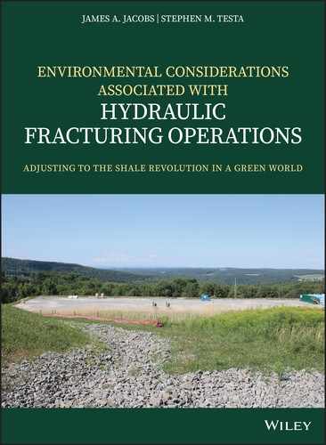
Dissolved flammable gases within the Bakken crude oil are released into the vapor space of rail tank cars as the ambient temperature increases. In the event of a spill or catastrophic release, the gases trapped in the rail tank car vapor space increase flammability and inhalation hazard risks. The main hazard associated with Bakken crude oil in a rail accident is flammability, resulting in explosions, fireballs, and pool fires. A major aboveground tank rupture or pipeline leak may result in an explosion and fireball after the spilled Bakken crude oil vaporizes and contacts an ignition source. A photo of the Casselton, North Dakota, fireball shows the explosion in process (Figure 15.2). The pileup of Bakken crude oil tanker cars south of Aliceville, Alabama, (US EPA 2013b) shows the extent of the derailment into the wetland environment (Figure 15.3).
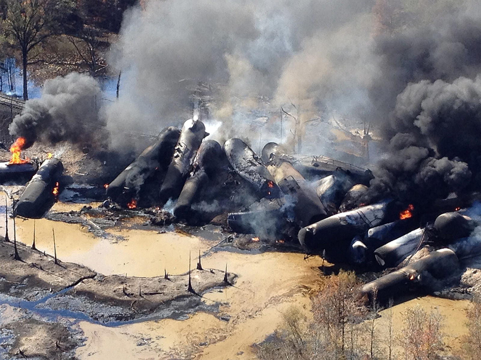
Figure 15.2 On 8 Nov 2013, a train carrying Bakken crude oil derailed south of Aliceville, Alabama, into the adjacent wetlands. The derailment caused 23 tanker cars to be derailed; many were caught on fire and several of the cars were breached. (US EPAOSC 2013).
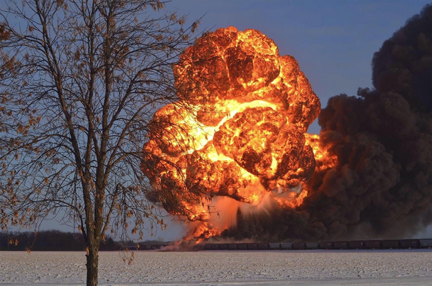
Figure 15.3 A massive fireball followed the derailment and explosion of two unit trains, one carrying 106 cars of Bakken crude oil in Casselton, North Dakota, on 30 December 2013 (US Pipeline and Hazardous Materials Safety Administration 2013).
15.3.3 Summary of Bakken Crude Oil Spill Incidents
Bakken crude oil rail accidents are summarized in Table 15.9 (MassDEP 2015).
Table 15.9 Summary of rail accidents.
| Rail accident and date | Date | Description | Volume | Outcome |
| Lac‐Mégantic, Quebec | 7/6/13 | A Canadian Pacific Railway 74 runaway train derailment of (63) 30 000 gal (114 m3) railcars containing Bakken crude oil en route to the Irving Oil Refinery in St. John’s New Brunswick, Canada | About 1.7 million gal (6435 m3) were either burned or released into the environment with an estimated 26 000 gal (98 m3) spilling into the nearby Chaudière River. Oil flowed in storm sewers, manholes, basements, and other subsurface conduits or structures. About 150 000 cy (114 683 m3) soil removed and 50 million gal (189 271 m3) water treated |
|
| Aliceville, Alabama | 11/7/13 | Derailment of Alabama and Gulf Coast Railway 25 train, 23 breached into wetland. Train was carrying 2.7 million gal (10 221 m3) of Bakken crude oil | 630 000 gal (2 385 m3) of crude oil either spilled or burned. 11 000 gal (41.6 m3) oil was recovered and 5 000 US tons (4 536 metric tons) of soil excavated from rail bed and adjacent wetland |
|
| Casselton, North Dakota | 12/30/13 | Eastbound BNSF Railway crude oil unit train with 106 cars collided with a westbound BNSF unit train carrying grain. The car collision caused 20 Bakken crude oil tank cars to derail. 18 were breached | 400 000 gal (1 514 m3) of crude oil was released |
|
| Lynchburg, Virginia | 4/30/14 | CSXT 13‐unit cars of a 105‐car train derailed; 3‐unit cars submerged in James River | 30 000 gal (114 m3) released, 3 cars submerged in the James River |
|
| Plaster Rock, New Brunswick | 1/7/14 | 19‐unit cars of a Canadian National Railway 122 unit freight train derailed with 9 Bakken crude oil units and liquefied petroleum gas (butane and propane). Two unit tank cars were breached, resulting in the fire | A defective wheel caused the derailment of the train. Older tank cars were punctured by couplers. About 60 760 gal (230 m3) of Bakken crude oil spilled fueling a massive fire (Abdelwahab 2015). 5000 tons (4536 metric tons) of impacted soil were removed |
|
| Luther, Oklahoma | 8/22/08 | 14 unit cars of a BSNF 110 car train carrying Bakken crude oil derailed. 3 unit cars breached and remainder leaked crude | 80 746 gal (305.6 m3) released, 3 cars breached remainder leaked and caught fire |
|
| Parker Prairie, Minnesota | 3/27/13 | 14‐unit cars of a Canadian Pacific 94 car unit train derailed. 1 car breached and 2 additional cars leaked while on their side following derailment | 30 000 gal (113.5 m3) released on to frozen soil |
|
15.3.4 Fate and Transport of Spilled Crude
The major migration pathways from a surface Bakken crude oil spill from a rail accident or tank failure (Table 15.10) might include a variety of media to sample depending on the active processes ().
modified after MassDEP (2015)
Table 15.10 Processes, media, and recommended sample type for oil spills.
| Process | Media | Sample type |
| Evaporation | Into air | Air samples |
| Volatilization | ||
| Dispersion | ||
| Infiltration | Into soil | Soil and soil vapor samples |
| Direct surface release | Into streams, rivers, lakes, coastal waters, outer harbors, open water ditches, wetlands | Water and soil samples |
| Leaching from shallow soil | Into groundwater | Groundwater samples |
| Transport in groundwater | Migration in groundwater | |
| Partitioning between media (API 2001, 2005, 2011) | Characteristics | Sample type |
|
|
Air samples |
| Water samples | ||
|
|
Air samples |
| Water samples | ||
| Water samples | ||
| Water samples | ||
| Soil samples | ||
|
|
Soil samples |
| Activity | Critical data | Example decisions |
| Spill emergency response | Volume of the released oil | Type of equipment, staff, evacuation criteria |
| Type of crude oil – physical and chemical properties | Type of equipment | |
| Dispersal rate of crude oil | Type of equipment | |
| Receiving media (air, soil, and/or water) | Type of equipment, access | |
| Topography of the terrain | Movement of oil | |
| Weather, especially wind and temperature | Movement of oil | |
| Process of crude oil spill into water body | Description of process | Estimated process time (determined by site‐specific conditions) |
| Process | Forces | Stage |
| Spreading of crude oil on water (US EPA 2004) | Gravity and inertial forces control the spreading of crude oil across the surface | Stage 1 |
| Process of crude oil spill into water body | Inertial forces become negligible in comparison with viscous drag across the surface | Stage 2 |
| Process | Interfacial forces become dominant and are the driving force to propel oil spreading | Stage 3 |
| Dissolution | Water soluble portions of crude oil may dissolve into the surrounding water | Hours to days |
| Natural dispersion | Oil slick broken up by waves and turbulence | Hours to days |
| Emulsification | Water‐in‐oil emulsion formed from Bakken crude oil in water | Days to months |
| Biodegradation | Biologic consumption of spilled Bakken crude oil and by‐products that require food source, electron acceptor, and microbial communities | Optimal reaction rate days to years. Cold climates (Alaska) can retard biodegradation rates to decades |
| Photooxidation | Direct photooxidation: crude oil reacts chemically with oxygen in water or in the atmosphere either breaking down into soluble products or forming persistent compounds called tars | Reaction rates weeks to years |
| Emulsification | Indirect photooxidation (lighter crude oil portion, volatilize to air | Lighter crude oil portion will volatilize into air. Reaction rates days to months |
| Sedimentation and sinking | Heavier ends of Bakken crude oil will adhere to sediment | Days to years |
| Burning | Process | Duration |
| Combustion | Controlled and uncontrolled burning of crude oil from tank car spills | Hours to weeks |
15.3.5 Combustion
Intentional (or uncontrolled) burning of Bakken crude oil released during train accidents emits the following hazardous compounds into the air (Lemieux et al. 2004). Those compounds which are not shown in the table are sulfur dioxide, carbon monoxide, and particulates; these are common in Bakken crude oil emissions from burns (Table 15.11).
Table 15.11 Combustion of Bakken crude oil and estimated emissions.
Source: Lemieux et al. (2004).
| Compound | Emissions (mg kg−1 burned) |
| Benzene | 251 |
| Formaldehyde | 139 |
| Naphthalene | 44 |
| Benzo(a)pyrene | 1 |
| Total dioxins and furans | 0.000 428 |
15.3.6 DOT‐117 Tank Car Design
The 2013 train disaster in Lac‐Mégantic, Quebec, proved the need for improved safety in tank car design, while transporting Bakken crude and other flammable substances. Unlike in DOT‐111 tank cars, new regulations were developed effective 1 October 2015 for DOT‐117 tank cars, which feature improvements for unpressurized tank car design to transport flammable liquids such as crude oil and ethanol (DOT 2016; NTSB 2015; PHMSA 2017). The DOT‐117 (Figure 15.4) standard includes the following:
- Normalized steel heads and shields.
- ½‐in full head shields (full height).
- Tank material: head and shell thickness (9/16 in).
- Top fittings protection.
- ½‐in ceramic insulation.
- Steel jackets (complete).
- High flow pressure relief valve.
- Improved bottom outlet valve handle.
Figure 15.4 After 1 October 2015, DOT‐117 (TC‐117 in Canada) is the new standard for all new unpressurized tank cars in use on North American railroads. Photo of DOT‐117 tank car (NTSB 2015) (above). DOT‐117 diagram with improvements listed (below).
15.4 Violations
PADEP keeps records for administrative and environmental health and safety (ESH) violations. From 2009 to 2015, there have been thousands of violations (Table 15.12). The top 20 violations provide insight into the types of challenges operators are facing in maintaining best management practices such as creating and implementing a written erosion and sediment control plan (ESCP) when earth disturbance activities will affect an area of more than 5000 ft2 (465 m2) or more.
Table 15.12 Number and type of administrative, environmental, health, and safety violations.
Source: From PDEP (2017).
| Description of violation | Type of violation | Total number of violations | Total number of wells |
| Failure to properly store, transport, process, or dispose of a residual waste | Environmental health and safety | 490 | 401 |
| Oil and Gas Act (OGA) 223 – General. Used only when a specific OGA code cannot be used | Administrative | 349 | 183 |
| Failure to minimize accelerated erosion, implement erosion and sediment (E&S) plan, and maintain E&S controls. Failure to stabilize site until total site restoration under OGA Sec 206(c)(d) | Environmental health and safety | 315 | 251 |
| Failure to adopt pollution prevention measures required or prescribed by the Department of Environmental Protection (DEP) by handling materials that create a danger of pollution | Environmental health and safety | 292 | 246 |
| Failure to properly control or dispose of industrial or residual waste to prevent pollution of the waters of Pennsylvania | Environmental health and safety | 243 | 207 |
| Pit and tanks not constructed with sufficient capacity to contain polluting substances | Administrative | 222 | 193 |
| Failure to report defective, insufficient, or improperly cemented casing within 24 hours or submit plan to correct within 30 days | Administrative | 175 | 158 |
| Discharge of pollution to waters of the state | Environmental health and safety | 155 | 125 |
| Clean Streams Law (CSL) – General. Used only when a specific CSL code cannot be used | Administrative | 149 | 121 |
| Failure to post permit number, operator name, address, and telephone number in a conspicuous manner at the site during drilling | Administrative | 135 | 121 |
| Failure to maintain 2′ freeboard in an impoundment | Administrative | 107 | 82 |
| Failure to submit well record within 30 days of completion of drilling | Administrative | 100 | 98 |
| Failure to notify DEP of pollution incident. No phone call made forthwith | Administrative | 87 | 80 |
| Impoundment not structurally sound, impermeable, 3rd party protected, >20″ (51 cm) of seasonal high groundwater table | Administrative | 79 | 69 |
| E&S plan not adequate | Administrative | 70 | 64 |
| Improperly lined pit | Administrative | 70 | 61 |
| Failure to design, implement, or maintain best management practices (BMPs) to minimize the potential for accelerated erosion and sedimentation | Administrative | 69 | 53 |
| Failure to post pit approval number | Administrative | 64 | 63 |
| Failure to install, in a permanent manner, the permit number on a completed well | Administrative | 63 | 58 |
| Failure to plug a well upon abandonment | Administrative | 61 | 58 |
15.5 Forensic Analysis
Forensic analysis depends on information on the variations in chemical composition, physical attributes, or other factors that can differentiate contaminated water, soil, or gas samples from another. Forensic analysis is used in areas with unconventional oil and gas drilling and production activities, as well as rail accidents to identify the origin or source of contamination. Sometimes the answers to forensic analysis suggest that unconventional oil and gas operations are not causative or related to conditions in aging domestic water wells, but rather that natural conditions or native compounds such as methane or metals, such as iron, may contribute to the poor quality of domestic water. Other differentiating factors helpful to forensic analysis include the ratio of certain elements or compounds in two or more samples or the relationship between various isotopes in compared samples.
15.5.1 Gas Chromatograms
It has been estimated that an average crude oil has about 100 000 different compounds and the use of ultrahigh‐resolution mass analysis can separate and identify tens of thousands of these compounds (Marshall and Rodgers 2008). A gas chromatograph (GC), a primary tool in chemical laboratory business, can identify about 1000 compounds in crude oil. Chemists even use the term “fingerprint” evaluation for the forensic task of examining laboratory data to determine and differentiate sample sources, weathering, or other processes that may have modified sample characteristics. GCs have long been used to “fingerprint” crude oils for geochemical differentiation (McCaffrey et al. 2011, 2017). The number of possible analytes for coproduced water is exceedingly large (Figure 15.5). The relative abundance or ratios of specific elements or compounds and their isotopes to other analytes, the amount of weathering in a sample, or even the low concentrations of tentatively identified compounds (TICs) are all used in the multiple lines of evidence to identify the sources of hydrocarbons and other contaminants.
Figure 15.5 Coproduced water has a variety of chemical characteristics that might be used to help identify the source of the water (Hayes and Severin 2012).
15.5.2 Tentatively Identified Compounds (TICs)
Laboratory‐reported TICs from VOC and SVOC analyses can sometimes provide clues to the presence of chemicals, which may help to identify potential sources of contamination. TICs are compounds that can be detected by the laboratory analytical methods, but, without the analysis of standards, these chemicals cannot be confirmed or reliably quantified. To be identified as a TIC, a chromatogram peak has to have an area of at least 10% as large as the area of the nearest internal standard as well as a match quality >80% (US EPA 2015e). The TIC match quality is based on the number and ratio of the major fragmentation ions. A TIC value of 99 is a perfect match. Although the TIC report is essentially a qualitative report, an estimated concentration can be calculated based on a response factor of 1.00 and the area of the nearest internal standard. Frequently, TICs are representative of a class of compounds rather than indicating a specific compound (US EPA 2015e), and in some cases, TICs can be useful in providing diagnostic forensic information. An example might be a TIC of 2‐butoxyethanol (C6H14O2), a glycol ether that could be used as a hydraulic surfactant or foaming agent. Although the TIC indicates minute quantities below standard reporting levels, the presence of 2‐butoxyethanol can be important nonetheless. In the absence of other potential chemical sources, 2‐butoxyethanol could, with other lines of supporting evidence, provide a chemical source from HVHF operations. An example VOC analysis chromatogram shows four TICs identified: acetic acid, toluene, heptane, and D‐limonene (Figure 15.6). The joint presence or specific industrial uses of the TICs may help to provide evidence of the source of the contaminants.
Figure 15.6 Tentatively identified compounds (TICs) from this volatile organic compound (VOC) analysis lists chemicals with low concentrations, which might otherwise be missed. Example VOCs in this printout include acetic acid and D‐limonene, which have component retention times of 6.1480 and 11.2388 minutes, respectively.
15.5.3 Piper Diagrams
Specific ion chemistry, when plotted on a piper diagram, can be used to help differentiate between multiple sources of water, using anion and cation ratios (Figure 15.7; Table 15.13). The piper diagram shows data from the US EPA Northeast Pennsylvania retrospective case study (US EPA 2015a), which is described later in this chapter. Piper diagrams can frequently be used to identify water sources related to specific aquifers, fluids used in unconventional oil and gas operations, or waters used in agricultural or industrial activities, based on dissolved anions and cations. The three points of the cation plot (left side of Figure 15.7) are calcium, magnesium, and sodium plus potassium cations. The points of the anion plot are sulfate, chloride, and bicarbonate and carbonate anions. The two triangular‐shaped ternary plots are then projected upward onto a diamond plot. The diamond plot is a graph of the anions (sulfate and chloride/total anions) and cations (sodium and potassium/total cations). In this case, water containing different ratios of dissolved salts have been identified using the piper diagram.

Figure 15.7 Typical piper diagram showing cations and anions present in water.
Source: Data from the US EPA Northeast Pennsylvania retrospective case study US EPA (2015a).
Table 15.13 List of major ions, trace metals, nutrients, physical properties, selected analytical method, and detection limits.
Source: From Reilly (2014).
| Major cations | Method | Detection limit |
| Sodium – Na+ | EPA 200.7 | 0.05, 0.5 |
| Potassium – K+ | EPA 200.7 | 0.5 |
| Calcium – Ca2+ | EPA 200.7 | 0.01, 0.1 |
| Magnesium – Mg2+ | EPA 200.7 | 0.01, 0.1 |
| Barium – Ba2+ | EPA 200.7 | 0.01 |
| Strontium – Sr2+ | EPA 200.7 | 0.01 |
| Manganese – Mn2+ | EPA 200.7 | 0.01 |
| Iron – Fe2+ | EPA 200.7 | 0.01 |
| Aluminum – Al3+ | EPA 200.7 | 0.02 |
| Major anions | ||
| Chloride – Cl− | EPA 300.0 | 0.5, 0.9, 1 |
| Bromide – Br− | EPA 300.0 | 0.1 |
| Sulfate – SO42− | EPA 300.0 | 0.9, 1.8 |
| Trace metal | ||
| Arsenic – As | EPA 200.8 | 0.001 |
| Nutrients | ||
| Nitrate–nitrite as N | EPA 353.2 | 0.2, 0.3 |
| Total Kjeldahl nitrogen | SM 4500 Norg B/SM 4500 NH3 B&C | 0.84 |
| Total nitrogen | Calculation | 0.89 |
| Physical properties | ||
| Alkalinity as CaCO3 | EPA 310.2 | 2, 10 |
| Total dissolved solids | SM 2540 C | 5, 10, 20 |
15.5.4 Biomarkers
Biomarkers, complex molecules derived originally from formerly living organisms, are found in petroleum and include pristane, phytane, porphyrin, steranes, and triterpanes. There is little change in their structures where they are detected in the range of several hundred mg l−1 or parts per million (ppm) (Peters et al. 2007a, b). Biomarkers have been used for a variety of chemical fingerprinting studies relating to the origin of the petroleum, the types of the precursor organic matter in the petroleum source rock, the correlation of the crude oil with the organic material found in the source rocks, the environmental conditions of sediment deposition, the assessment of thermal maturity, the thermal history of the crude oil, the degree of biodegradation, the later alteration, and the information as to the age of the source rock (Fingas 2010).
Used as biomarkers for phytoplankton, isoprenoids pristane and phytane primarily originate from the phytol side chain of the chlorophyll molecule (Didyk et al. 1978; Volkman and Maxwell 1986) and their identification can be useful (Figure 15.8). Biomarker compounds are usually identified using gas chromatography‐mass spectrometry (GC‐MS) techniques. Although isoprenoids may comprise <5% of diesel fuel, these branched alkanes have a chemical structure that generally inhibits biodegradation, so they are usually preserved and can be relied upon as diagnostic compounds.
Figure 15.8 Biomarkers pristane and phytane are sourced from chlorophyll and are frequently preserved and present in crude oil and refined petroleum hydrocarbon products (Zafiriou et al. 1977).
15.5.4.1 Compound‐Specific Isotope Analysis
When organic compounds, including petroleum hydrocarbons, degrade in the environment, the ratio of stable isotopes will often change over time. Different leaks or spills of the same material at different times may have different isotopic fingerprints or signatures that can be used for identification. Weathering processes include evaporation, emulsification, adsorption, dispersion, dissolution, oxidation–reduction reactions, and biodegradation. Compound‐specific isotope analysis (CSIA) is the technique used to assess biodegradation and source identification of organic contaminants in groundwater (Hunkeler et al. 2008). The CSIA uses a GC with an isotope‐ratio mass spectrometer (GC‐IRMS) to better differentiate comingled plumes of the same chemical compounds (Figure 15.9).
Figure 15.9 GC‐IRMS is used for compound‐specific isotope analysis of carbon compounds (Hunkeler et al. 2008).
CSIA is based on the concept that atoms of a specific element must have the same number of protons and electrons, but they can have a different number of neutrons. When atoms differ only in the number of neutrons, they are referred to as isotopes of each other. If a particular isotope is not radioactive, it is called a stable isotope. Because they differ in the number of neutrons, a mass spectrometer is used to identify different isotopes of the same element, which differ in mass (Hunkeler et al. 2008). CSIA is also used to evaluate naturally occurring organic compounds such as aromatic compounds, diamondoids, isoprenoids, and n‐alkanes.
15.5.4.2 CSIA of Biomarkers
CSIA of biomarkers (CSIA‐B) is used for source correlation to determine the source of two or more crude oil mixtures. Although produced crude oil, nearby surface seeps, and crude oil generated from the original source rocks may have similar physical characteristics, CSIA‐B can be used to measure specific biomarker steranes and hopanes to differentiate the source.
15.5.5 Chemical and Biological Transformations
Some parent compounds, such as tetrachloroethene (PCE), tetrachloroethane (PCA), and 1,2‐dichloroethane (1,2‐DCA), show transformations related to biological or abiotic processes (Figure 15.10). These compounds are industrial cleaners and solvents.

Figure 15.10 Transformations of contaminants, in this case, chlorinated aliphatic hydrocarbons (NJEHD 2005).
A variety of compounds that are likely to be encountered at the well pad such as benzene, toluene, ethylbenzene, and xylene (BTEX) compounds are naturally found in crude oil as well as refined products such as gasoline, diesel, and kerosene. Sorption, volatilization, and other abiotic processes also transform chemicals over time. BTEX compounds can degrade with both the faster aerobic or slower anaerobic biodegradation pathways (Figure 15.11).

Figure 15.11 Dominant terminal electron‐accepting process, electron acceptors, and typical chemical species responses.
Source: From US EPA (2013c) as modified from AFCEE (2004) and Bouwer and McCarty (1984).
For an aerobic biodegradation process, benzene ultimately breaks down to carbon dioxide and water through this general process:
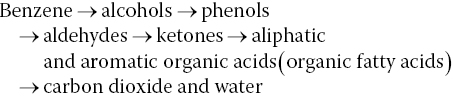
The co‐metabolic degradation pathway occurs when microbial communities using one compound as an energy source produce an enzyme that chemically transforms and degrades another compound present at the same location. In some cases, analytical chemistry such as US EPA Method 8260B/C GC‐MS and understanding redox conditions can be used to explain degradation products and the ratio of parent compound to degradation products. However, not all compounds can be identified by current laboratory analytical methods.
A variety of molecular diagnostic tools can identify microbial communities and site‐specific organisms. Direct DNA isolation from soil or water samples, denaturing gradient gel electrophoresis (DGGE), polymerase chain reaction (PCR) methods, enzyme activity probes (EAPs), and nucleic acid hybridization (NAH) are a few of the molecular biology techniques providing information on the biological communities in areas with contaminated soil or groundwater. Using these advanced biochemical diagnostic tools can enable more cost‐effective and efficient bioremediation, as well as providing more biochemical evidence of microbial activity in the subsurface and possible parent chemicals and source locations.
15.5.6 Chemical Ratios
Chemical ratios have been used successfully to distinguish among various sources of stray gas. There are multiple salinity sources in the environment (Vengosh et al. 2011), and detailed geochemistry is needed to evaluate the potential salt sources (Table 15.14). The household compound, sodium chloride (NaCl) or common table salt, also provides a good example of the complexities of source identification in the subsurface. For example, the ratio of bromide/chloride (Br/Cl) to chloride can be used to differentiate among background groundwater, groundwater affected by septic sources, and groundwater affected by road salt, backflow, and brine waters (Kight and Siegel 2011).
Table 15.14 Chemical ratios to identify salt sources.
Source: From Vengosh et al. (2011).
| Salt sources | Water type | Chemical compositions |
| Road salt deicing | NaCl water type | Na/Cl ratio = 1 |
| Br/Cl ratio is low | ||
| B/Cl ratio is low | ||
| Domestic waste water and septic tanks | NaCl water type | Na/Cl ratio is ≥1 |
| NO3 is high | ||
| Br/Cl ratio is low | ||
| B/Cl ratio is high | ||
| Acid mine drainage | CaSO4 water type | B/Cl ratio is high |
| pH is low | ||
| Natural saline groundwater | Depends on water type source | Ratios vary on source |
| Coal ash leachates | CaSO4 water type | High Ca, High pH |
| B/Cl ratio is very high | ||
| High‐volume hydraulic fracturing (HVHF) fluids | Depends on water type source; salts added | High Ca, Sr, B, Ba concentrations |
| Marcellus brines | CaCl water type | Na/Cl ratio is <1 |
| Br/Cl ratio is high | ||
| B/Cl ratio is high |
15.5.7 Geochemical Tracers
Geochemical tracers are a specific substance used to trace the course of a process. It may be an element or compound that can be tracked and identified throughout chemical or biological processes by its chemical characteristics such as unusual isotopic mass, radioactivity, or inert behavior. An ideal geochemical tracer may have some of the following characteristics (Lalor and Pitt 1999):
- It can be detected at low concentrations.
- Small variations in tracer concentrations can be differentiated between two or more water sources.
- Tracers generally have stable behavior, so concentrations of the tracer do not attenuate much over time due to physical, chemical, or biological processes.
- A tracer is diagnostic of specific processes or from particular water sources.
- There is an ease of measurement with adequate detection limits.
- Tracers generally accepted standard method of analysis.
- Good sensitivity and repeatability for the tracer tests.
For hydraulic fracturing specialty chemical additives, some of the specific synthetic organic compounds can be used as tracers. However, due to the proprietary nature of many of the chemical additives as well as harsh geochemical conditions in deep shale basin environments, there may be few chemical additives that can serve as tracers.
15.5.7.1 2‐n‐Butoxyethanol Tracer Case Study
Foaming domestic water wells nearby a Marcellus Shale well pad were described in one case near Marcellus Shale gas wells in Pennsylvania. To figure out the source of the foam, samples of almost 30 flowback fluids or coproduction waters were provided, from unconventional natural gas wells drilled in the Marcellus Shale, before treatment at a brine wastewater remediation plant. A sample of drilling foam (M‐I SWACO Platinum Air Foam) from a Schlumberger company was obtained and analyzed. And samples from several domestic wells and a spring were obtained and analyzed (Llewellyn et al. 2015).
One compound in flowback fluids, 2‐n‐butoxyethanol (2‐BE; Chemical Abstracts Service (CAS) number 111‐76‐2), was positively identified in one of the domestic water wells containing an unidentified foaming agent at nanogram‐per‐liter concentrations. The same compound was also identified in the drilling additive and surfactant AirFoam HD. Compound 2‐BE was detected using a new analytical technique, comprehensive 2D gas chromatography coupled to time‐of‐flight mass spectrometry (GCxGC‐TOFMS). Although it does provide an ultralow detection capability, the analytical method is not common or commercially available (Llewellyn et al. 2015).
There have been no reports showing 2‐BE as a naturally occurring compound in waters from the area (Leenheer et al. 1982). In a study of 4 wells in the area, one nearby domestic water well contained about 0.42 ng l−1 2‐BE before purging, and another well contained about 0.086 ng l−1 2‐BE after purging; No 2‐BE was detected in the other two groundwater wells. A few of the 30 flowback/production water samples were positively identified as containing 2‐BE (Llewellyn et al. 2015). There are other industrial sources of 2‐BE besides its use at unconventional oil and gas well sites. A fully miscible, clear liquid with an ether‐like odor at thresholds of 0.10–0.40 ppm in air, 2‐BE is also used as an industrial solvent for paints and surface coatings and is an ingredient for paint thinners, cosmetics, degreasers, dyes, soaps, and herbicides (Llewellyn et al. 2015). In this case, chemicals like 2‐BE could be potentially used as geochemical tracers. The source of the ng l−1 concentrations of 2‐BE foaming agent in the domestic water wells would require more analysis and multiple lines of evidence.
15.5.8 Isotopes
Isotopes are natural variations of a specific element that contains equal number of protons but different number of neutrons in their nuclei, thus isotopes of the same element have varying relative atomic mass but have almost identical chemical properties.
15.5.8.1 Hydrogen and Oxygen Isotopes
Stable isotopes of water are measured as the ratios of the two most stable and abundant isotopes of each element. Most hydrogen (1H) atoms have 1 proton and no neutrons for an atomic weight of 1. The relative abundance of 1H is 99.9885%. Heavy hydrogen, which is the less common isotope of the lightest element (0.0115% relative abundance), also called deuterium (2H or D), has 1 proton and 1 neutron for an atomic weight of 2. Tritium of 3H has 2 neutrons and 1 proton for an atomic weight of 3. Hydrogen also has isotopes from 4H to 7H, which are rare and unstable, but 1H and 2H represent virtually 100% of all hydrogen atoms. The stable isotope ratio of hydrogen is the ratio of 2H (0.0115% of all hydrogen atoms) to 1H (99.9885% of all hydrogen atoms). The 2H/1H ratio is about 0.000 115.
Most oxygen atoms (99.757%) are 16O, which has 8 protons and 8 neutrons for an atomic weight of 16. Heavy oxygen (18O) has 8 protons and 10 neutrons for an atomic weight of 18. Heavy oxygen has a relative abundance of 0.205%. There are other isotopes of oxygen (for example17O), but 16O and 18O represent 99.962% of all oxygen atoms. The stable isotope ratio of oxygen is the ratio of the less common 18O (0.205% of all oxygen atoms) to the more common 16O, which includes 99.757% of all oxygen atoms. The 18O/16O ratio is about 0.002 055.
15.5.8.2 Carbon and Methane Isotopes
Carbon isotopes are notated as δ13C and pronounced “delta carbon thirteen.” Schoell (1980) showed that the ratio of heavy hydrogen (deuterium) (δ2H CH4); 0/00 (relative to Vienna Standard Mean Ocean Water (VSMOW)) compared with carbon (δ13CCH4); 0/00 (relative to Vienna Pee Dee Belemnite (VPDB)) could be used to differentiate methane samples based on origin. The methane source zones based on hydrogen and carbon isotope data from dozens of researchers were compiled (Coleman et al. (1993) based on data from Schoell (1980)). Thermogenic methane derived from the Marcellus Shale has a relatively consistent carbon to hydrogen isotopic ratio (Figure 15.12). Other stable isotope data using carbon and hydrogen isotopes from north central and northeast Pennsylvania (Baldassar 2011a, b) show background stray gas from the northeastern Pennsylvania in Potter, Tioga, Bradford, and Chemung counties (and from the literature) to display much greater variability than the methane sourced from the Marcellus Shale (Saba 2013). Forensic methods have been developed to differentiate methane sources (Table 15.15).
Figure 15.12 Carbon vs. hydrogen isotopes: biogenic and thermogenic methane.
Source: Saba (2013); used by permission.
Table 15.15 Forensic methods to differentiate methane sources.
| Microbial methane acetate fermentation: marsh gas and landfill gas | ||
| Isotope | Fraction | Range |
| Carbon 13C | δ13C of CH4 | −40 to −62 0/00 |
| Heavy hydrogen (deuterium) | δ2H of CH4 | −270 to −350 0/00 |
| Microbial methane: CO2 reduction called drift gas | ||
| Isotope | Fraction | Range |
| Carbon 13C | δ13C of CH4 | −62 to −90 0/00 |
| Heavy hydrogen (deuterium) | δ2H of CH4 | −180 to −240 0/00 |
| Thermogenic methane: natural gas from the shale gas sources | ||
| Isotope | Fraction | Range |
| Carbon 13C | δ13C of CH4 | −26 to −50 0/00 |
| Heavy hydrogen (deuterium) | δ2H of CH4 | −110 to −250 0/00 |
A stable carbon isotope relates to the gas sample, compared with the standard, as in the following equation (Saba 2013):
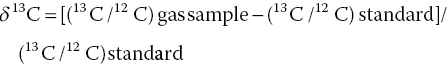
The stable carbon isotope of methane is expressed as parts per thousands (0/00). δ13C will vary in time related to depositional history: vegetation type, productivity, and organic carbon content and burial. The standard for δ13C is Vienna Pee Dee Belemnite (VPDB). Collected from the banks of the Pee Dee River in South Carolina, the original Pee Dee Belemnite (PDB) contained extinct fossilized belemnite shells. Since the original rock sample has been consumed completely through analysis, other reference standards were calibrated to the original PDB sample. Carbon isotope values are still reported relative to PDB using the term “VPDB” to show the values that have been normalized to the standard. The standard for δ2H is the oxygen ratios that are measured are compared relative to Vienna Standard Mean Ocean Water (VSMOW). Isotopic compositions of both oxygen and hydrogen are reported against the VSMOW standard.
15.5.9 Forensic Isotope Analysis
A wide variety of other available soluble isotopes, such as lithium, boron, strontium, radium, and others, can undergo forensic analysis. These available soluble isotopes are used in unconventional oil and gas source studies. Isotopic forms have been discovered for every element, and there are 275 isotopes of the 81 stable elements and over 800 radioactive isotopes (Thomas 2013). The isotope abundance measurements are obtained from Rosman and Taylor (1999). Stable isotopic analysis has been used to evaluate stable isotopes in the water cycle (Gat and Gonfiantini 1981) as well as differentiate rainwater (Dansgaard 1964), groundwater (Gat 1971), and surface water (Muir and Coplen 1981).
Isotope mass and abundance is described in Henderson and McIndoe (2005). Dissolved isotope chemical analysis is used in unconventional resource studies and source identification (Table 15.16). Using the dissolved isotopes for forensics is based on the theory that stable isotopes for water such as oxygen δ18O and hydrogen δ2H and dissolved salt isotopes such as boron 11B/10B, strontium 87Sr/86Sr, and radium 228Ra/226Ra in shale waters differ from those in shallow groundwater, surface water, or other water sources.
Table 15.16 Selected isotopes used in differentiating sources of water or methane related to unconventional oil and gas operations.
| Isotope name | Chemical symbol | Mass of atom (u) | % abundance | No. of neutrons | No. of protons |
| Hydrogen (protium) | (1H) | 1.007 825 | 99.9885 | 0 | 1 |
| Deuterium | (2H, or D) | 2.014 102 | 0.0115 | 1 | 1 |
| Tritium | (3H, or T) | 3.016 049 | Not available | 2 | 1 |
| Lithium‐6 | 6Li | 6.015 121 4 | 7.59 | 3 | 3 |
| Lithium‐7 | 7Li | 7.016 003 0 | 92.41 | 4 | 3 |
| Boron‐10 | 10B | 10.012 936 9 | 19.9 | 5 | 5 |
| Boron‐11 | 11B | 11.009 305 4 | 80.1 | 6 | 5 |
| Carbon‐12 | (12C) | 12 | 98.93 | 6 | 6 |
| Carbon‐13 | (13C) | 13.003 354 826 | 1.07 | 7 | 6 |
| Carbon‐14 | (14C) | 14.003 242 | Not available | 8 | 6 |
| Nitrogen‐14 | 14N | 14.003 074 002 | 99.632 | 7 | 7 |
| Nitrogen‐15 | 15N | 15.000 108 97 | 0.368 | 8 | 7 |
| Oxygen‐16 | 16O | 15.994 914 63 | 99.757 | 8 | 8 |
| Oxygen‐17 | 17O | 16.999 131 2 | 0.038 | 9 | 8 |
| Oxygen‐18 | 18O | 17.999 160 3 | 0.205 | 10 | 8 |
| Sulfur‐32 | 32S | 31.972 070 70 | 94.93 | 16 | 16 |
| Sulfur‐33 | 33S | 32.971 458 43 | 0.76 | 17 | 16 |
| Sulfur‐34 | 34S | 33.967 866 65 | 4.29 | 18 | 16 |
| Sulfur‐36 | 36S | 35.967 080 62 | 0.02 | 20 | 16 |
| Chlorine‐35 | 35Cl | 34.968 852 72 | 75.78 | 18 | 17 |
| Chlorine‐35 | 37Cl | 36.965 902 62 | 24.22 | 20 | 17 |
| Bromine‐79 | 79Br | 78.918 336 1 | 50.69 | 44 | 35 |
| Bromine‐80 | 80Br | 80.916 289 | 49.31 | 46 | 35 |
| Strontium‐84 | 84Sr | 83.913 430 | 0.56 | 46 | 38 |
| Strontium‐86 | 86Sr | 85.909 267 2 | 9.86 | 48 | 38 |
| Strontium‐87 | 87Sr | 86.908 884 1 | 7.00 | 49 | 38 |
| Strontium‐88 | 88Sr | 87.905 618 8 | 82.58 | 50 | 38 |
| Lead‐202 | 202Pb | Unstable | Not available | 120 | 82 |
| Lead‐204 | 204Pb | 203.973 020 | 1.4 | 122 | 82 |
| Lead‐206 | 206Pb | 205.974 440 | 24.1 | 124 | 82 |
| Lead‐207 | 207Pb | 206.975 872 | 22.1 | 125 | 82 |
| Lead‐208 | 208Pb | 207.976 627 | 52.4 | 126 | 82 |
| Radium‐226 | 226Ra | 226.025 403 | 100 | 138 | 88 |
| Radium‐228 | 228Ra | 228.031 063 | Trace | 140 | 88 |
15.5.10 Boron and Strontium Isotope Ratios
Some researchers have shown that the Marcellus Shale has a δ11B value of 32–33‰ and a 87Sr/86Sr value of 0.7115. These values, obtained from the Catskill Formation in eastern Pennsylvania, differ from shallow groundwater isotope values of 13.1–28.1‰ for δ11B and 0.712 01–0.715 53 for 87Sr/86Sr (Saba 2013). Based on these distinct ratios of boron, lithium, strontium, and selected other isotopes, flowback fluid of unconventional oil and gas operations can frequently be differentiated from the conventional coproduced water and water from other sources. These characteristics make these elements boron and lithium, which frequently occur naturally in shale formations useful in forensic analysis. When unconventional oil and gas operators inject hydraulic fracturing fluids under high pressure into a black organic‐rich shale formation, not only are the petroleum hydrocarbons released, but also soluble elements such as boron and lithium that are attached to clay minerals within the shale formation are also released during the HVHF operations. Boron and lithium are carried to the surface mixed in with the flowback fluids. Boron and lithium have distinctive isotopic fingerprints and are stable both in the deep shale basin and at the surface, making them suitable as forensic tracers. Boron (B), lithium (Li), and chloride (Cl−): [B/Cl, Li/Cl, δ11B vs. δ7Li] are useful in characterizing the flowback fluids from other water sources. In a study based on 39 hydraulic fracturing flowback fluids and coproduced water samples from the Marcellus and Fayetteville black shale formations (Warner et al. 2014), the ratio of B/Cl (>0.001), Li/Cl (>0.002), δ11B (25–31 ‰), and δ7Li (6–10 ‰) compositions of the flowback fluids was distinct in most cases from the coproduced waters collected from conventional oil and gas wells. Certain elements or compounds are more likely to be identified with flowback fluids. To reinforce the use of these elements in forensic work, a comparison of general isotope ratios of boron and lithium (Table 15.17) was used effectively to differentiate conventional coproduced water from seawater, unconventional HVHF flowback fluid from unconventional oil and gas operations, and global river waters (Warner et al. 2014).
Table 15.17 General isotope ratios of boron and lithium illustrate the general concept of produced fluid differentiation.
Source: Concept and data based on Warner et al. (2014).
| Source of water | δ11B (0/00) | δ7Li (0/00) |
| River water | 10 | 20 |
| HVHF flowback water | 27 | 10 |
| Seawater | 39 | 31 |
| Conventional coproduced water | 46 | 16 |
Values are approximate.
15.5.11 Radioactive Isotopes
Isotopes of radioactive elements have been analyzed as part of the evaluation of naturally occurring radioactive materials (NORM) and technologically enhanced naturally occurring radioactive materials (TENORM) at unconventional and conventional oil and gas fields. NORM and TENORM are generally in sludges, wastes, or by‐products which is enriched with radioactive elements such as radium, uranium, thorium, and potassium and the associated decay products. US EPA regulates radionuclides based on concentration in liquids in micrograms/liter (μg l−1) or parts per billion (ppb). A picocurie, or pCi, is a standard measure of the intensity of radioactivity or how frequently a radioactive particle is released in a sample of radioactive material. The background levels of NORM in Pennsylvania measured in groundwater ranged from <0.1 to 167 picocuries per liter (pCi l−1) for gross alpha (α), 0.6–270 pCi l−1 for gross beta (β), and <0.6–172 pCi l−1 for combined radium (Saba 2013; USGS 2000). These ranges contain background concentrations greater than US EPA’s maximum contaminant levels (MCLs) of 15, 4, and 5 pCi l−1 for gross alpha, beta, and combined radium, respectively. Generally, NORM samples should be collected, and the concentrations should be compared with MCLs and background levels. In other cases where NORM values have been established, the NORM background levels even in oil and gas production areas are well below MCLs.
Marcellus Shale flowback fluids and coproduced waters from gas production wells in central and western Pennsylvania show elevated concentrations of 226Ra and 228Ra in some of the flowback brines, with total 226Ra+228Ra concentrations ranging from 73 to 6540 pCi l−1; these concentrations exceed US EPA’s MCL (5 pCi l−1) by 13–1300 times (US EPA 2015b; Haluszczak et al. 2013; Rowan et al. 2011). Gross radioactivity and specific radionuclides including gross α radioactivity, gross β radioactivity, and the radium isotopes 226Ra and 228Ra were evaluated in southwest Pennsylvania by US EPA (2015b). The main α emitting radionuclides in the natural decay series are 238U, 234U, 230Th, 226Ra, 210Po, 232Th, and 228Th. The major β emitting radionuclides are 210Pb, 228Ra, and 40K (Bonotto et al. 2009). US EPA (2015b) noted that naturally occurring radioactivity in groundwater is produced primarily by the radioactive decay of 238U and 232Th. Having a half‐life of 4.5 × 10⁹ years, the 238U atom and its decay series products include 226Ra and 222Rn. Flowback fluids or coproduced waters may contain some level of background radioactive elements, as in the case of the Marcellus Shale (US EPA 2015b). Levels of radioactivity and specific radioactive isotope ratios can be used to evaluate whether flowback fluids or coproduced waters have mixed with shallow groundwater or surface water resources.
Radium‐containing barite, called radiobarite, has been a documented constituent of some scale and sludge deposits that are generated in oil and gas field production equipment (Zielinski et al. 2001). Radium‐bearing saline formation water pumped to the surface along with crude oil can form a barite precipitate on production equipment surfaces. Age estimates can be calculated based on their decay: short‐lived 228Ra has a half‐life of 5.76 years, which is short compared to the significantly longer half‐life of 1600 years for 226Ra. Present activity ratios of 228Ra/226Ra in radiobarite‐rich scale or highly contaminated soil are compared with initial ratios at the time of radiobarite precipitation. Radium isotopes can be used to determine the age and source of radioactive barite at oil field production sites (Zielinski et al. 2001). Radioactivity levels in some oil field equipment and in soils contaminated by radium‐bearing scale and sludge can be high enough in some cases to pose a potential health threat, and evaluation of site‐specific data reduces the risks of uncertainty. Radioisotope information can be used to help identify water or fluid sources.
15.5.12 Case Studies
In a variety of case studies, included below, isotopic analysis, chemical ratios, other forensic information, and multiple lines of evidence are used to identify sources of water or contamination.
| Location | Main study | Target zone | Counties |
| North California | Ulrick (2017) | Marcellus Shale | Various |
15.5.12.1 Water Isotope Case Study in Northern California
A stable isotope water study in the San Francisco Bay area of northern California was conducted by Jim Ulrick (2017) to differentiate water sources that included tap water, recycled water, rain water, and water from swimming pools. Over a period of 14 years, Ulrick collected 181 water samples for stable isotope ratio analyses. Monthly rainfall samples were also collected for volume‐weighted composite 2012 water‐year stable isotope values. An additional 28 isotope ratios of water from selected water sources from the area were compiled from data in other reports (Muir and Coplen 1981; Newhouse et al. 2004).
In the Ulrick study, a sample stable isotope ratio is measured and compared to the VSMOW, an internationally known reference. Delta (δ) notation is used to show the difference between the sample and VSMOW measurements. The δ values are expressed as parts per thousand or per mil (‰) because the differences are minute. For example, a positive δ value of +10 ‰ for oxygen (δ18O = +10 ‰) means that the sample is enriched in 18O by 10 ‰ compared to VSMOW. The δ18O and δ2D% ratios of precipitation worldwide vary as a function of temperature, elevation, and latitude, and plot along the global meteoric water line (GMWL) (Figure 15.13).
Figure 15.13 Stable isotope ratios of water to differentiate water sources.
Source: After Ulrick (2017); used by permission.
Main Findings: The five sources of water are clearly differentiated based on the ratio of heavy oxygen enrichment compared with heavy hydrogen enrichment (Ulrick 2017).
15.5.12.2 Water Isotope Case Study in Northeast Pennsylvania
| Location | Main study | Target zone | Counties |
| Northeast Pennsylvania | Reilly (2014) | Marcellus Shale | Tioga, Bradford, Lycoming, and Sullivan |
A geochemical study (Reilly 2014; Reilly et al. 2015) was performed using stable isotope analysis of groundwater samples collected in 2012–2013 from 21 groundwater wells in Tioga, Bradford, Lycoming, and Sullivan counties in northeastern Pennsylvania. The groundwater wells were identified by their owners as possibly being contaminated from nearby unconventional gas operations. Water samples from the 21 wells were compared with geochemical data from historical groundwater, Marcellus Formation flowback fluids, and other sources of contaminated waters (Reilly 2014; Reilly et al. 2015). The water analyses included sodium (Na), potassium (K), calcium (Ca), magnesium (Mg), barium (Ba), strontium (Sr), manganese (Mn), iron (Fe), aluminum (Al), chloride (Cl), bromide (Br), sulfate (SO4), arsenic (As), nitrate–nitrite as N, total Kjeldahl nitrogen, total nitrogen, alkalinity, and TDS.
Road salt, animal waste, septic effluent, and Marcellus Formation flowback fluids (Figure 15.14) plotted on a trilinear diagram (piper plot) show that the flowback fluids are limited to areas on the chart that can be identified based on the specific pattern.
Figure 15.14 A Cl/Br vs. Cl cross‐plot with all data points and group averages, along with groundwater 2 Standard Deviation lines marked with the mean and a mark on the chloride axis indicating the secondary maximum contaminant level (250 mg l−1).
Source: After Reilly (2014); used by permission.
The study found that the cause of the 21 well owner complaints was related to natural geochemical conditions in the aquifer or, in the case of one well and possibly others, was impacted by either septic effluent or animal waste. Earlier water sampling studies in the area in 1980 showed 11% of groundwater samples to be impacted by septic effluent. The ion concentrations from the 21 wells did not exceed US EPA primary or secondary contaminant levels and were within the range established during the groundwater study performed in 1980 in the area. Common exceedances in water quality were related to the natural geochemistry of the Catskill and Lock Haven aquifers, which are naturally high in manganese and iron (Reilly et al. 2015).
Main Findings: The study concluded that no evidence exists that groundwater in the 21 wells tested was impacted by Marcellus Formation drilling, hydraulic fracture operations, or gas production activities. The study showed that water well owner complaints in the study area are not uncommon and aquifer qualities related to naturally occurring dissolved minerals such as iron or manganese can impact water quality, as can the conditions of the water wells and proximity to animal wastes and fecal matter. Based on the reaction of well owners to hydraulic fracturing operations in the general area, better communication and information transfer between the operators, regulatory agencies, and the public are needed (Reilly et al. 2015). Improvements to water well quality can be accomplished by understanding the well water chemistry and through regular well maintenance such as well redevelopment, chlorination practices, or water treatment.
15.6 Prospective and Retrospective Case Studies
Prospective case studies involve evaluation of areas that have not yet been drilled and are not impacted by other industrial processes to determine whether oil and gas development contaminates groundwater and surface water resources. Prospective case studies are designed to allow sampling and characterization of a site before, during, and after drilling and hydraulic fracture operations, including the full water cycle: water acquisition, drilling, hydraulic fracture operations, fluid injection, flowback, and coproduction of fluids and gases. Prospective studies tend to take longer to complete, are usually costlier, and may have less bias than retrospective case studies. Generally, prospective case studies follow the following development (Ford and Briskin 2013):
- Site selection.
- Baseline monitoring.
- HVHF well pad installation.
- HVHF well drilling and completion.
- Hydraulic fracturing.
- Flowback management.
- Oil–as production and coproduced waste management.
A water quality monitoring project for a prospective case study would be designed to sample nearby downgradient private wells and surface water bodies (Figure 15.15) before drilling or industrial activities would commence. Baseline sampling is a key component of case studies. A new constructed network of monitoring wells could be placed in locations that would intercept potential groundwater flow from the well pad to downgradient receptors. The monitoring wells installed in different aquifers could obtain local information such as individual groundwater zone depth and preferred flow pathways, flow rates, and flow directions. Data from field meters/kits and laboratory analytical tests should be regularly collected to evaluate changes in water quality over time and assess the fate and transport of potential chemical contaminants. Although two prospective case studies were originally planned by US EPA, the studies were eventually canceled.

Figure 15.15 Conceptual model for prospective case study near an HVHF well pad (no scale implied).
Source: Modified after Ford and Briskin (2013).
In contrast with prospective case studies, retrospective case studies involve studying areas where potential impacts of an activity, such as hydraulic fracture operations, have occurred and some level of impact has been noted. The studies may evaluate data and determine whether or not the hydraulic fracture operations are the cause of potential impacts to water resources. Historic oil and gas production operations have occurred in areas where unlined mud pits may have been used or other releases may have occurred. Isolating the environmental impacts of fluid releases from new drilling activities and processes from historic practices can be difficult. Retrospective case studies frequently lack baseline data, such as site‐specific water quality data, which is useful to correlate water resource impacts with definitive causes or sources. Even with these types of limitations, potential vulnerabilities to water resources can still be described.
15.6.1 US EPA Retrospective Case Study
Congress urged US EPA to study the relationship between HVHF operations and potable water resources in December 2009. US EPA planned for retrospective case studies by asking stakeholders across the nation to participate in identifying specific locations for potential case studies. From comments provided at US EPA meetings as well as electronic or written concerns or complaints from the public, over 40 possible locations were nominated for inclusion in the US EPA research. Possible case study locations were prioritized based on US EPA criteria, including proximity of the case study location to the population and drinking water supplies, the amount of reported evidence of water quality impacts, environmental and health concerns, and information gaps that could be filled at each possible case study location. The US EPA also wanted the selected case study areas to represent diversity in the following categories:
- Geographic and geologic characteristics.
- Populations at risk.
- Hydrogeologic and water resource conditions.
- Land uses.
US EPA reviewed the information and finalized five case study areas where hydraulic fracture operations have already occurred and alleged examples of water resource contamination are well documented. The five case study locations (Figure 15.16) included two sites in Pennsylvania, one site in Texas, one site in Colorado, and one site in North Dakota (Table 15.18).
Figure 15.16 Locations of US EPA retrospective case studies and associated hydrocarbon reservoirs (US EPA 2015a, b, c, d, e).
Table 15.18 Summary of US EPA case study locations.
| US EPA case study location | Unconventional reservoir | Counties |
| Northeast Pennsylvania | Marcellus Shale | Bradford and Susquehanna |
| Southwest Pennsylvania | Marcellus Shale | Washington |
| North Texas | Barnett Shale | Wise and Denton |
| West North Dakota | Bakken Shale | Dunn (largest town: Killdeer) |
| Southeast Colorado | Raton Basin Coalbed methane | Las Animas and Huerfano |
The examples of water quality concerns used for the selection of the five case study sites were based on complaints, which were typical of the types of issues that were reported to the agency during the 2010 and 2011 stakeholder meetings. Water and air quality degradation complaints can be related to industrial activities or possibly other causes such as biological, geochemical, or structural processes. The US EPA study with five retrospective sites was planned to evaluate the complaints and to try to correlate the key factors that could be associated with the frequency and severity of alleged drinking water quality degradation from hydraulic fracture operations.
The US EPA examined five operations of the hydraulic fracturing water life cycle:
- Water acquisition – possible impacts related to large‐volume surface or groundwater extraction.
- Chemical mixing – possible environmental impacts at the well pad.
- Well injection – possible impacts related to the injection of specialized chemicals and hydraulic fracturing on water resources.
- Flowback and coproduced fluids and gases – possible impacts of surface spills or subsurface leakage and migration of fluids or gases into beneficial use aquifers and surface water sources.
- Wastewater treatment and waste disposal – possible impacts of incomplete treatment of wastes on water sources.
The US EPA retrospective case study program started with a project study plan (US EPA 2011a) based on extensive stakeholder outreach in five areas undergoing unconventional oil and gas development with horizontal drilling combined with hydraulic fracture operations. The study plan was developed with a large number of stakeholders, including other federal agencies, state and interstate regulatory agencies, nongovernmental organizations (NGO), the oil and gas industry, and others in the public and private sectors. The study plan underwent a peer review process by the EPA Science Advisory Board (SAB), which assembled an independent panel of experts for final comments and review.
15.6.2 US EPA Retrospective Study Approach and Sampling Activities
US EPA researchers compiled historic water quality databases and public information about drilling and hydraulic fracture operations, conducted detailed literature reviews, and analyzed historical background or baseline geology and hydrology data for each of the five case study locations. US EPA collected water samples from the summer of 2011 until the spring of 2013 from a variety of sources, including domestic wells, water supply wells, municipal wells, production wells, groundwater monitoring wells, and surface water sources during multiple sampling trips to the five case study locations. Field water quality parameters were monitored and documented during water sample collection (Table 15.19). Although variations exist, water analyses conducted by US EPA in the five retrospective case studies generally included most of these analyte groups (Table 15.20). Dissolved inorganic carbon (DIC) is the sum of all the carbonate species present such as carbonate and bicarbonate dissolved in water.
Table 15.19 Summary of US EPA field parameters used in retrospective case studies.
Source: Modified after Wilkin (2013) and US EPA (2015a, b, c, d, e).
| Parameters | ||
| pH (units) | Water temperature (°F or °C) | Turbidity (NTU) |
| Total dissolved solids (TDS; mg l−1) | Dissolved oxygen (DO; mg l−1) | Oxidation/reduction potential (ORP; mV) |
| Specific conductance (S m−1) | Alkalinity (mg l−1 of CaCO3) | Water depth (ft or m) |
| Dissolved hydrogen sulfide (HS; mg l−1) | Dissolved ferrous iron (Fe2+; mg l−1) | |
Table 15.20 Analyte groups and example constituents.
Source: Modified after Wilkin (2013) and US EPA (2015a, b, c, d, e).
| Analyte groups | Examples |
| Anions (major and trace) | Bromide (Br−), chloride (Cl−), sulfate (SO4−2) |
| Carbon group | Dissolved organic carbon, dissolved inorganic carbon1 |
| Cations (major and trace) | Calcium (Ca), magnesium (Mg), potassium (K), and sodium (Na) |
| Dissolved gases | Methane, ethane, propane, n‐butane |
| Dissolved carbon | Dissolved organic carbon (DOC); dissolved inorganic carbon (DIC) |
| Elements, trace | Arsenic (As), barium (Ba), iron (Fe), manganese (Mn), selenium (Se), and strontium (Sr) |
| Extractable petroleum hydrocarbons | Gasoline range organics (GRO; C5–C12) |
| Diesel range organics (DRO; C15–C18) | |
| Glycols | Diethylene glycol, triethylene glycol, tetraethylene glycol, and 2‐butoxyethanol |
| Isotopes | Isotopes of oxygen and hydrogen in water, carbon, and hydrogen in methane, strontium |
| Low molecular weight acids | Lactate, formate, acetate, butyrate, propionate, and isobutyrate |
| Radioactive species and radioactivity | Radium‐226, radium‐228, gross alpha activity, and gross beta activity |
| Stable isotopes | (δ13CCH4, δ2HCH4,δ13CC2H6,δ13CDIC,δ18OH2O, δ2HH2O, and 87Sr/86Sr) |
| Semivolatile organic compounds (SVOCs) | Benzoic acid; 1,2,4‐trichlorobenzene; 4‐nitrophenol |
| Surfactants | Octylphenol ethoxylate, nonylphenol |
| Volatile organic compounds (VOCs) | Benzene, ethylbenzene, toluene, xylenes (BTEX), styrene, ethanol, isopropyl alcohol, tert‐butyl alcohol, naphthalene, and chlorinated solvents (including industrial cleaners and degreasers) |
US EPA examined water sources where homeowner‐specific complaints indicated environmental concerns or where groundwater quality anomalies existed in the vicinity of unconventional gas wells. Example complaints of water quality included increased turbidity, effervescing, discoloration, staining, and odor. US EPA performed the retrospective case study to determine whether water quality concerns or anomalies could be attributed to the nearby hydraulic fracture operations or other activities.
15.6.2.1 Northeast Pennsylvania Case Study
| Location | Main study | Target zone | Counties |
| Northeast Pennsylvania | US EPA (2015a) | Marcellus Shale | Bradford and Susquehanna |
US EPA (2015a) studied groundwater wells, springs, ponds, and streams in Bradford and Susquehanna counties (Figure 15.17) in northeastern Pennsylvania. Northeastern Pennsylvania oil and gas exploration and production began as early as the 1860s. The Marcellus Formation is a Middle Devonian shale with an age of about 390 million years (Figure 15.18). The Marcellus Shale is a black, low density, and high organic carbon content. It occurs in the subsurface beneath much of New York, Pennsylvania, Ohio, and West Virginia, as well as in smaller areas of Virginia, Kentucky, Maryland, and Tennessee. In Bradford and Susquehanna counties in northeastern Pennsylvania, the Marcellus Shale lies about 4000–8000 ft (1219–2438 m) below the surface and ranges in thickness from about 150 to 300 ft (46–91 m). The Marcellus Shale is part of a transgressive sedimentary package formed by the deposition of terrestrial and marine material in a shallow, inland sea. The Marcellus Shale is underlain by the sandstones and siltstones of the Onondaga Formation and overlain by laminated shales, siltstones, and fine‐grained sandstones of the Mahantango Formation (US EPA 2015a). Aquifers in the area, notably the Devonian Catskill Formation rocks and the overlying Pleistocene glacial till aquifers, provide water sources (see Figure 15.18). Potable fresh groundwater occurs to depths of about 200 ft (61 m) in the valleys and about 800 ft (244 m) below ground surface in the upland areas. The average depth to groundwater in northeast Pennsylvania is about 175 ft (53 m) below ground surface but is frequently <40–50 ft (12–15 m) below the surface in the valleys (Battelle 2013). Generally, below the zone of fresh water, groundwater has elevated salinity, although shallow saline sources have been documented in the lowlands (Williams et al. 1998). The depth and thickness of the Marcellus Shale generally increases from northwest to southeast and near Bradford and Susquehanna counties; the formation is about 4000–7000 ft (1219–2134 m) below ground surface (Battelle 2013).

Figure 15.17 The case study sample location map for Bradford County, Pennsylvania, showing surface water, domestic well, and spring water sample locations (US EPA 2015a).

Figure 15.18 Generalized stratigraphic column (above) in northeast Pennsylvania.
Source: Modified after Berg et al. (1983) and US EPA (2015a).
A generalized east–west cross section (below) for northeast Pennsylvania.
Source: Modified after US EPA (2015a).
US EPA selected the initial sampling locations during an area reconnaissance conducted in August 2011 (Wilkin 2013) and analyzed for over 225 constituents including a large range of organic and inorganic constituents (US EPA 2015a). Sampling was conducted primarily in the southern portion of Bradford County, Pennsylvania. Sampling in the adjacent Susquehanna County was limited to three homeowner wells. Collectively, a total of ~100 drilled gas wells, most of which were hydraulically fractured, were within 5280 ft (1609 m) of the water sampling locations in the study, except for one well. Historic water quality data from before 2007 and before Marcellus Shale gas extraction in this area was obtained by US EPA from a literature search and from the US Geological Survey (USGS), National Water Information System (NWIS), and National Uranium Resource Evaluation (NURE) databases.
The number of water samples per sampling event ranged from 23 to 35. The US EPA study consisted of three rounds of water sampling and laboratory analyses conducted over a span of less than two years (Table 15.21).
Table 15.21 Northeast Pennsylvania data source summary.
Source: Data from US EPA (2015a).
| Round | Date | Total number of samples | Wells | Springs | Ponds | Streams |
| Round 1 | Oct–Nov 2011 | 35 | 33 | 2 | 0 | 0 |
| Round 2 | Apr–May 2012 | 27 | 22 | 1 | 2 | 2 |
| Round 3 | May 2013 | 23 | 22 | 1 | 0 | 0 |
The level of shale gas drilling activity in Bradford County during the US EPA study (October 2011 to May 2013) has increased greatly as shown on the cumulative drilled oil and gas well diagram (Figure 15.19). Approximately 98% of drilled wells in Bradford County are unconventional wells, and over 99% are gas wells. Approximately 94% of wells as of July 2013 were classified as active based on the Pennsylvania Department of Environmental Protection (PADEP 2015) database for year 2013 (US EPA 2015a). A closeup map around the town of Towanda, Pennsylvania, in Bradford County shows the plan view orientation of the horizontally drilled gas well laterals (Figure 15.20) and some of the US EPA sampling locations. Some of the horizontally drilled gas wells shown on the map were drilled but not yet fractured by 12 February 2012, according to data supplied by Chesapeake Energy.
Figure 15.19 Diagram of drilled oil and gas wells in Bradford County since January 2000 showing totals starting in July 2008 extending to July 2013 (US EPA 2015a).
Figure 15.20 Map showing north–northwest and south–southeast orientation of gas well laterals in Towanda area of Bradford County as of February 2012 (US EPA 2015a).
Chemical Ratios: Bromide is a potential indicator of HVHF operations and was detected above the method quantitation limit (MQL) (1.0 mg l−1) at only 3 of the 38 groundwater locations sampled in the US EPA study (US EPA 2015a) and at none of the surface water locations. The ratio of chloride/bromide weight ratio compared with that of chloride in mg l−1 (Figure 15.21) shows differentiation of three groundwater wells compared with the more saline salt spring and Marcellus Shale flowback fluids. The National Uranium Resource Evaluation (NURE) 1977 groundwater data was used in the US EPA (2015a) Case Study. The figure shows a theoretical mixing curve with end members based on published data (Haluszczak et al. 2013; US EPA 2015a, using NURE 1977 data) of average flowback fluid chloride and bromide concentrations. Bradford County NURE chloride and bromide averages are 8.05 mg l−1 (n = 164) and 0.0231 mg l−1 (n = 112), respectively. NURE bromide data are for bromine analyzed by neutron activation analysis. Although there are only three groundwater samples, they can be separated from the flowback fluids based on these chemical ratios.
Figure 15.21 Chloride/bromide weight ratio to chloride (mg l−1) provides differentiation of three groundwater samples with detectable concentrations from Salt Spring or the Marcellus Shale flowback fluids (US EPA 2015a).
Methane: Dissolved methane in groundwater is ubiquitous in the area. According to the US EPA (2015a), stray gas migration is associated with the increased HVHF operations in this study area. This evidence comes from laboratory data that show changes in gas concentrations and/or the ratios of methane to ethane before and after unconventional gas drilling. Additional data from gas isotopes appear to show gas in some water wells is consistent with gas originating from deeper formations. Stray gas is encountered at almost all depths down to the Marcellus Formation, and according to US EPA, most of the stray gas originates from shallower formations. Based on isotope studies, elevated methane gas in the tested water wells was generally thermogenic in origin. The increased pace of unconventional gas activities in the study area has coincided with an elevated number of documented stray gas migration incidents (US EPA 2015a).
Stray gas is not unique to the current HVHF operations in northeast Pennsylvania. Baldassare (2011a, b) and Baldassare and Laughrey (1997) used geochemical and isotopic fingerprinting techniques to identify sources of stray gas. Stray gas commonly occurs within historic oil and gas basins. Methane gas occurs naturally in many water wells in the area at concentrations above both PADEP action level of 7 mg l−1. The Office of Surface Mining Reclamation and Enforcement (OSMRE) of the Department of Interior recommended an action level of 10 mg l−1, especially in groundwater rich in sodium bicarbonate (NaHCO3) and sodium chloride (NaCl). Concentrations of methane <10 mg l−1 in water or about 1–3% by volume in air are not generally a health or explosion concern but should be monitored to verify that the methane levels are not increasing (Eltschlager et al. 2001). At standard atmospheric pressure and at 68 °F (20 °C), dissolved methane in water can reach concentrations of 28 mg l−1. Elevated methane concentrations occur when fluids or water are extracted from higher‐pressure conditions at depth, and the dissolved gas comes out of solution as bubbles during a reduction in pressure.
Stray gas can pose an explosion risk if the gases accumulate in confined spaces or traps. Stray gas is also known to increase TDS and discoloration in well water. The sustained presence of methane in water wells can promote reducing conditions, changing geochemical conditions to lead to reductive dissolution of certain metals such as iron, manganese, and, to a lesser degree in this study area, arsenic. Stray gas also contributes to supporting methanotrophs, ubiquitous microbes in soils, sediment, and groundwater. Methanotrophs metabolize methane as their source of carbon and energy and can co‐metabolize many aliphatic compounds, alkanes, and aromatic compounds.
15.6.3 Main Findings
- The US EPA (2015a) performed extensive laboratory analysis of inorganic and organic compounds in up to 35 sample locations of alleged groundwater impacts, which were possibly linked to HVHF operations. Based on multiple lines of evidence, the US EPA report indicated no evidence of groundwater impacts related to hydraulic fracturing and the extraction of gas from the Marcellus Shale. The laboratory detections of inorganic and organic constituents in water samples could not be attributed to HVHF operations.
- Low concentrations of trimethylbenzenes (TMB) were present near or below MQL at two homeowner locations.
- Toluene was detected below the MQL in one groundwater sample, which was attributed to anthropogenic sources.
- Locally elevated natural background levels of TDS, chloride, sodium, barium, strontium, and combined radium‐226 and radium‐228 were known to occur in a few wells in certain valley areas.
- Related to natural aquifer geochemistry, iron and/or manganese concentrations exceeded secondary maximum contaminant levels (SMCLs) at over 40% of the groundwater locations.
- An anomalously high concentration of sulfate (>1000 mg l−1) was reported in 1 well, which may relate to the presence and dissolution of gypsum, a naturally occurring mineral in the area. The Marcellus Shale flowback and coproduced waters generally have sulfate concentrations <100 mg l−1.
- US EPA noted that stray gas, as methane and ethane, was present in 9 of the 36 water wells tested.
15.6.3.1 Southwest Pennsylvania Case Study
| Location | Main study | Target zone | Counties |
| Southwest Pennsylvania | US EPA (2015b) | Marcellus Shale | Washington |
Washington County lies in the southeast corner of Pennsylvania within the Appalachian Basin. Oil and gas exploration and production has a long history in Washington County, extending back to the late 1800s. The organic‐rich Devonian Marcellus Shale ranges in thickness from <50 ft (15 m) to about 150 ft (46 m) and varies in depth from about 5000 ft to over 7000 ft (1524–2134 m) below land surface.
Shallow domestic water wells are completed in the Quaternary alluvium, while deeper bedrock aquifers include the Permian Dunkard Group, Pennsylvanian Monongahela Group, and Conemaugh Group formations (Figure 15.22). Freshwater aquifers in some locations of Washington County, Pennsylvania, have been contaminated by brine from deeper, non‐potable aquifers through historical oil and gas wells that were improperly abandoned or have corroded casings (Newport 1973).
Figure 15.22 The case study sample location map for Washington County, Pennsylvania, showing water sample locations (US EPA 2015b).
Water sampling was conducted in Washington County, Pennsylvania (Figure 15.23), based on homeowner complaints or health concerns about water quality in potable wells. The domestic wells sampled in Washington County as part of the US EPA Retrospective Study (US EPA 2015b), ranged in depth from 50 to 160 ft (15–49 m) below land surface, with a median depth of 95 ft (29 m) below land surface. US EPA analyzed for over 235 constituents in water samples in Washington County (US EPA 2015b). Historic water quality data from before 2005 and before Marcellus Shale gas extraction in this area was obtained by US EPA from a literature search and from USGS, NWIS, and NURE databases.

Figure 15.23 Generalized stratigraphic column in southwest Pennsylvania.
Source: Modified after Berg et al. (1983) and US EPA (2015b).
The number of water samples per sampling event ranged from 15 to 16. The US EPA study consisted of three rounds of water sampling and laboratory analyses conducted in over a span of less than two years (Table 15.22).
Table 15.22 Southwest Pennsylvania data source summary.
Source: Data from US EPA (2015b).
| Round | Date | Total number of samples | Wells | Springs | Surface water |
| Round 1 | Jul 2011 | 16 | 12 | 1 | 3 |
| Round 2 | Mar 2012 | 15 | 10 | 3 | 2 |
| Round 3 | May 2013 | 15 | 11 | 2 | 2 |
The water samples were analyzed for over 235 target analytes, relating to local land use activities, as well as chemicals used in unconventional oil and gas drilling and production operations. Many of the types of exceedances in water quality goals in the retrospective case study conducted by the US EPA in Washington County, Pennsylvania, (Table 15.23) generally reflect natural sources of iron and manganese, natural sources of lead, nitrate from septic system or animal wastes, and dissolved methane from drift mine gas or coal seams (US EPA 2015a). Although specific spills or incidents related to HVHF operations may impact a nearby well or surface water source, as in the case of the drilling impoundment, widespread impacts to water resources were not reported by the US EPA (2015b).
Table 15.23 Summary of water quality exceedances for Washington County, Pennsylvania.
Source: From US EPA (2015b).
| Impacted parameters | Number of samples | Sample type | Description | Potential sources |
| Dissolved methane | 6 | Groundwater and springs | Detections from 0.002 to 15.5 mg l−1; consistent with biogenic and/or mixed biogenic and thermogenic sources | Drift gas; coal seams; long‐term migration from deep shales, sandstones, and coalbeds |
| Nitrate | 1 | Groundwater | Primary MCL exceedance | Septic systems; animal manure; fertilizers |
| Total lead | 2 | Groundwater | Primary MCL exceedance | Natural sources; pipes and/or solder corrosion |
| Iron and manganese | 8 | Groundwater, springs, surface water | Secondary MCL exceedances | Natural sources; turbidity potentially influenced by drilling; coal mine drainage |
| Aluminum | 7 | Groundwater and springs | Secondary MCL exceedances | Natural particulates; mineral content |
| Chloride | 4 | Groundwater, springs, surface water | Elevated concentrations compared to historical data; secondary MCL exceedances at one spring | Historical land use; current and/or historical drilling practices; impoundments; reserve pits; natural sources of brine; road salt |
Chemical Ratios: In southwestern Pennsylvania, chemical ratios were used to distinguish coproduced water from oil and natural gas production from various coal‐mine related wastewaters and brine treatment plant discharges. The chemical ratios used sulfate/chloride (SO4/Cl) weight ratios instead of bromide (Br) concentrations in mg l−1 (Wilson et al. 2014). The plot of the sulfate/chloride weight ratio compared with the bromide concentration (Figure 15.24) for surface water and shallow groundwater can be differentiated from the Marcellus Shale flowback water (data from Haluszcak et al. 2013), oil and gas brines from Pennsylvania (data from Dresel and Rose 2010), abandoned mine drainage, coal‐fired power plant effluent, and Marcellus Shale coproduced water (Wilson 2014). The sulfate/chloride weight ratio is generally elevated in coal‐related wastewaters than in oil and gas coproduced waters. The yellow shaded zones (see Figure 15.19) have been established by Wilson and others (2014). Bromide concentrations are also much higher in co‐produced waters from oil and gas production than in coal mine discharge. Bromide levels in surface water and groundwater were generally orders of magnitude lower than the bromide concentrations in Marcellus Shale coproduced water (US EPA 2015b).

Figure 15.24 Sulfate/chloride weight ratio compared with bromide concentration (mg l−1) for surface water and groundwater, as well as Marcellus Shale flowback fluids, oil and gas brines, and other water types (US EPA 2015b). CFPP, coal‐fired power plant.
Methane: Background chemical data from the US EPA study showed that methane is naturally occurring in this area and was detected in 24% of the groundwater and spring samples at concentrations ranging from about 0.002 to 15.5 mg l−1. US EPA noted that the isotopic signature of the methane present in domestic wells did not correlate well with the methane gas produced from the hydraulically fractured Marcellus Shale (US EPA 2015b). Methane occurs naturally in groundwater in Washington County, Pennsylvania, and is present in the subsurface down to the Marcellus Shale.
Main Findings:
- Elevated concentrations of chloride in groundwater was documented by the US EPA (2015b) at locations near a drilling mud pit site, which contained HVHF fluid wastes and drilling wastes. Based on multiple lines of evidence, US EPA concluded that the chloride contamination at sampling locations near one specific drilling mud pit was likely sourced from the impoundment itself.
- Washington County groundwater and surface samples contained no detections of acetate, GRO compounds, or glycol ethers, which might be associated with HVHF operations.
- Detections of VOCs and SVOCs were infrequent in the Washington County US EPA retrospective case study and were below US EPA’s drinking water MCLs.
- Although the primary MCL exceedances were noted at one location for nitrate and at two locations for total lead, the presence is not related to HVHF operations.
- US EPA noted that secondary MCL exceedances for manganese and iron were common in domestic wells, a reflection of naturally occurring conditions. Higher concentrations of manganese and iron reflect moderately, reducing groundwater conditions.
- Methane is naturally occurring and ubiquitous in groundwater in the area.
15.6.3.2 North Texas Case Study
| Location | Main study | Target zone | Counties |
| North Texas | US EPA (2015c) | Barnett Shale | Wise and Denton |
The US EPA studied Wise County for a north Texas retrospective study (Figure 15.25). The Barnett Shale (Figure 15.26), within the Bend Arch–Fort Worth Basin, is a Mississippian Shale with an age of about 320–360 million years ago. The Barnett Formation is widespread regionally within the basin, and recent unconventional gas production is relying on horizontal drilling and HVFS technologies to create fracture porosity, permeability, and gas flow. Wise County groundwater has been characterized as primarily calcium bicarbonate and sodium bicarbonate types, although occasionally other water types have been reported (US EPA 2015c).
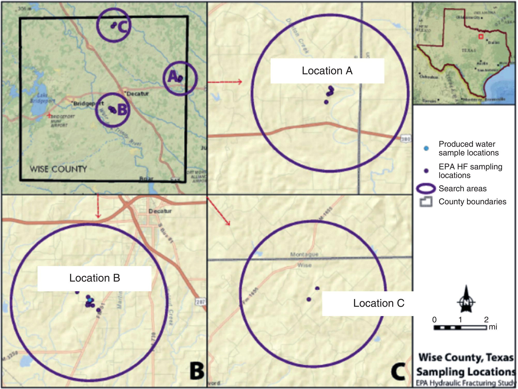
Figure 15.25 Detailed view of the Wise County sampling locations (US EPA 2015c).
Figure 15.26 A generalized stratigraphy column for the Fort Worth Basin. A, aquifer. B, Barnett Shale.
Source: Modified from Montgomery et al. (2005) and Bruner and Smosna (2011); as appeared in US EPA (2015c).
The Trinity aquifer (see Figure 15.26) is the primary source of drinking water in Wise County and 15 of 16 water wells in the US EPA retrospective case study were screened in that aquifer except for one well that was screened in an alluvial deposit. In addition to the 16 domestic wells, 4 surface water bodies at 3 locations within Wise County (locations A, B, and C) were sampled (Table 15.24). One of the surface water bodies sampled was a pond at location A and was the site of a reported March of 2010 fish kill. The study also included three gas production wells sampled by the US EPA: two of the gas wells which were sampled were completed within the Barnett Shale, and one gas well sampled for coproduced water was completed in the overlying Boonesville Bend Conglomerate formation.
Table 15.24 North Texas data source summary.
Source: Data from US EPA (2015c).
| Round | Date | Total number of samples | Wells | Surface water | Coproduced water (gas wells) |
| Round 1 | Sep 2011 | 16 | 13 | 3 | 0 |
| Round 2 | Mar 2012 | 18 | 15 | 3 | 0 |
| Round 3 | Sep 2012 | 4 | 3 | 0 | 1 |
| Round 4 | Dec 2012 | 10 | 9 | 1 | 0 |
| Round 5 | May 2013 | 15 | 8 | 5 | 2 |
Five sampling events have occurred, and in the Wise County study, the number of water samples per event ranged from 4 to 18. The water samples were analyzed for over 235 constituents relating to local land use activities, as well as chemicals used in unconventional oil and gas drilling and production operations.
15.6.3.2.1 Historical Databases
The US EPA data (2015c) was compared with historical water quality data documented in the literature, geochemical data in Texas Water Development Board (TWDB) database, and three national water quality databases: USGS, NWIS, and NURE. These sources provided data for water samples collected prior to 1993 (except NWIS), a time before the Barnett Shale was an HVHF gas target. The NWIS database only contains 1994 data for Wise County.
There are no DRO and GRO sample tests in the historical databases. The historical databases include SVOCs testing, but none were detected in the area. The historical databases showed that most of the trace elements, except for arsenic, iron, and manganese, were not detected or were found in very low concentrations. Arsenic, iron, and manganese concentrations in groundwater from the US EPA retrospective study were similar to the historical database concentrations, suggesting natural aquifer conditions. Naturally occurring, iron and manganese in groundwaters did exceed the US EPA SMCLs. Arsenic did not exceed the maximum contaminant level (MCL) (US EPA 2015c).
Methane
Dissolved methane was detected in 64% of the samples with methane concentrations in groundwater ranging from 0.0007 to 0.0242 mg l−1 and a median concentration of 0.0016 mg l−1. The low concentrations of dissolved methane were generally too low for isotopic analysis (US EPA 2015c). The Trinity aquifer outside of the specific US EPA study area contained dissolved methane levels that ranged from 0.0144 to 0.0347 mg l−1 (Zhang et al. 1998). Methane levels in both studies of the Trinity aquifer indicate the likely range of background methane levels, which naturally exist in the Trinity aquifer.
Main Findings:
- Concentrations of organic compounds in the Wise County samples did not exceed any US EPA drinking water standards when they were detected. In addition, there were no repeated detections in any water samples of any organic compounds associated with HVHF activities. Low concentrations in surface water of DRO compounds, VOCs, and SVOCs were detected at some sample locations during a few of the sampling events. GRO compounds were detected in one groundwater sample, and an SVOC (bis‐(2‐ethylmethyl) phthalate) was detected in two wells (US EPA 2015c).
- In up to 6% of the water sample, VOCs were detected at concentrations below US EPA drinking water standards. The detected VOCs included benzene, which occurred in 6% of the detections, 1,2,4‐trimethylbenzene occurring in 2% of the detections, tert‐butyl alcohol, methyl tert‐butyl ether (MTBE), ethyl tert‐butyl ether, tert‐amyl methyl ether, m–p‐xylenes, and o‐xylene. Some of these compounds are linked to a proximity of vehicles and generators near the sampling activities. Other potential sources of VOCs were not identified.
- The study was broken into three study areas (A, B, and C), and in two out of the three study locations, there were no impacts to groundwater. In the third study area, two domestic wells had elevated levels of chloride, specific conductivity, calcium, potassium, magnesium, sodium, bromide, iodide, and strontium, likely from formation brines. Chloride was noted to exceed the SMCL by 2.2–7.9 times. A third well located at an industrial facility was identified as potentially impacted by brines and/or landfill leachate. Several sources for impacts from formation brines were identified, but specific potential pathways were not determined.
- Glycol ethers, compounds commonly found at well sites during HVHF operations or associated with other industrial processes, were not detected in surface or groundwater samples.
- Methane in the study area is naturally occurring based on the widespread occurrence of dissolved methane in groundwater from the Trinity aquifer.
15.6.3.3 West North Dakota Case Study
| Location | Main study | Target zone | Counties |
| West North Dakota | US EPA (2015d) | Bakken Shale | Dunn |
The US EPA Killdeer study area is the location of historical oil and gas production, as well as current unconventional oil production from the Bakken Shale. The US EPA case study near Killdeer, North Dakota, was designed to evaluate the potential impacts to drinking water resources related to a known oil well blowout, which occurred during HVHF operations in September 2010. The blowout released crude oil, hydraulic fracturing fluids, and flowback fluids onto the surrounding area. Cleanup efforts were started after the blowout. Various state agencies were involved, including the Division of Water Quality (NDDWA) of the North Dakota Department of Health and the Oil and Gas Division of the North Dakota Industrial Commission (NDIC). US EPA was requested by these agencies to perform a retrospective case study at the Killdeer blowout site. US EPA set out to determine whether drinking water resources, including the Quaternary Killdeer aquifer, were impacted from the blowout event with associated fluid surface spill, which occurred at the Franchuk 44‐20 SHW well (Figure 15.27).
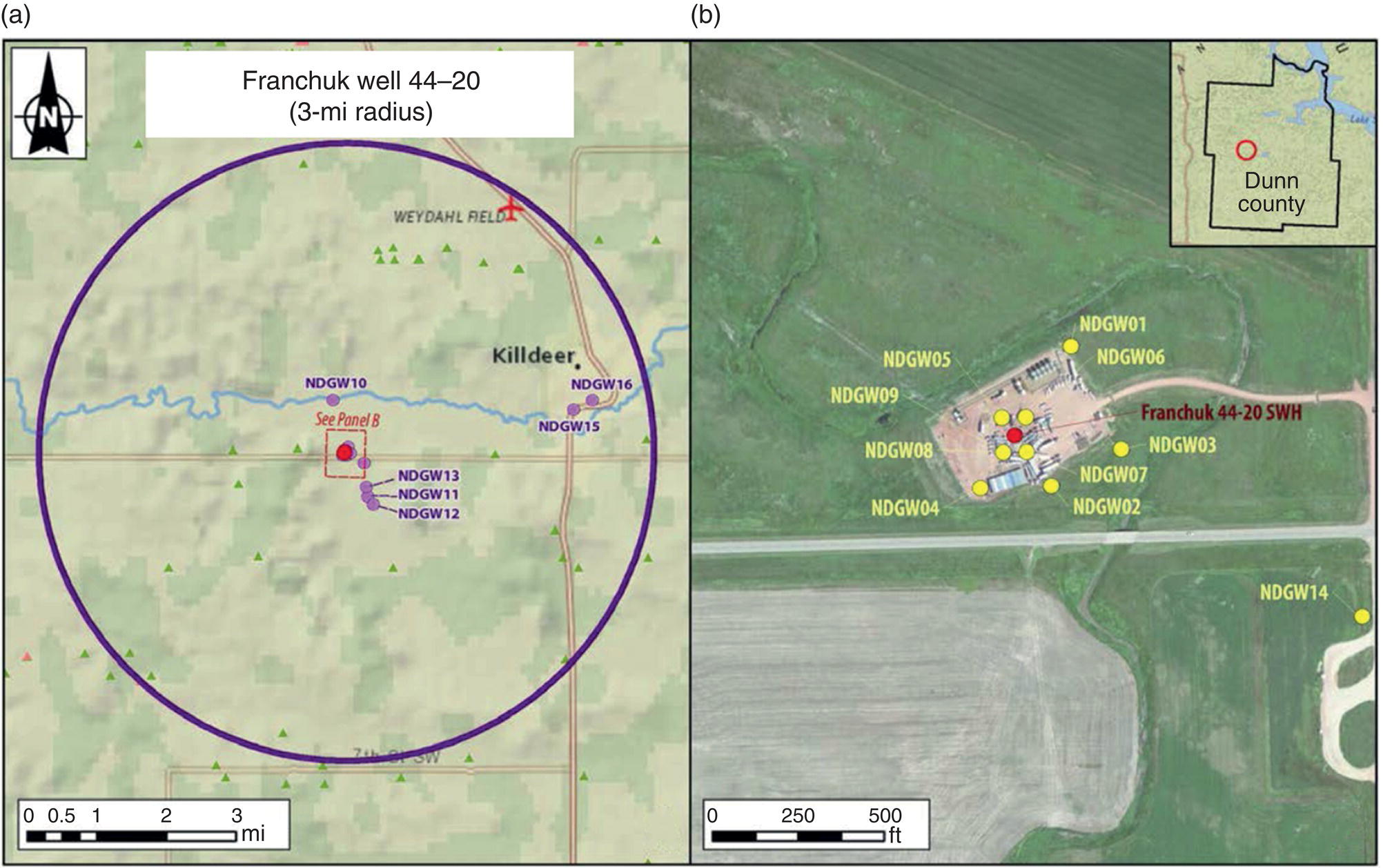
Figure 15.27 Killdeer retrospective case study locations. (a) Shows the 3‐mi radius and gives the locations of the non‐pad wells sampled as part of this study. (b) Shows a zoomed in view of the well pad and gives the locations of the pad wells sampled as part of this study (US EPA 2015d).
Dunn County is situated on the Missouri Slope uplands of the Great Plains region of western North Dakota. The general geology of Dunn County consists of thick sequences of Cenozoic, underlain by Mesozoic, and older Paleozoic rocks, which have accumulated in the Williston Basin (Figure 15.28). Approximately 7500 ft (2,286 m) of Paleozoic rocks underlie Dunn County (Murphy 2001), including the Late Devonian to Early Mississippian organic‐rich deep marine Bakken Shale deposited ~400 million years ago. The Bakken Shale consists of an upper and lower organic‐rich deep marine shale deposited under anoxic conditions, separated by a middle dolomite member. The estimated top of the Precambrian crystalline rocks ranges from 11 000 to 13 400 ft (3 353–4 084 m) below sea level in Dunn County (Heck 1988; Heck et al. 2013; Murphy 2001).
Figure 15.28 Stratigraphic column for Dunn County, North Dakota.
Source: Aquifer information from Klausing (1976, 1979); figure modified from Murphy (2001).
Nearby Aquifers: Deeper wells in the area which may produce from rock aquifers (from bottom to top) include the Cretaceous Hell Creek and Fox Hills formations and Tertiary Ludlow, Cannonball, Tongue River, and Sentinel Butte formations (Klausing 1976, 1979). Overlying the Tertiary rocks, the Quaternary alluvium aquifers in Dunn County are found in sediments that were deposited before glaciation and within areas of glacial deposits, which consist of till and glacio‐fluvial sand and gravel deposits that are confined to glacial meltwater channels and include the Killdeer, Horse Nose Butte, Knife River, and Goodman Creek aquifers. The primary water source underlying the Franchuk 44‐20 SHW well is the unconfined to semiconfined Killdeer aquifer (Figure 15.29) consisting of fine to course gravel near the base overlain by a predominantly fine to medium sand, which generally lies below clay and silt deposits (Klausing 1976). The Killdeer aquifer has a maximum thickness of 233 ft (71 m) and an average thickness of 80 ft (24 m). The Killdeer aquifer recharges by infiltration of rainwater. The depth to water during the US EPA study ranged from 19.8 to 33.6 ft (6.0–10.2 m) below ground surface (bgs) (US EPA 2015d). Water extracted from the Killdeer aquifer is generally hard and is characterized as either sodium bicarbonate type or sodium sulfate type of water (Klausing 1976). The groundwater flow direction is to the southwest and has a relatively uniform gradient of 0.0009–0.0008, which varies seasonally depending on water usage and precipitation.
Figure 15.29 Generalized cross section of the shallow Killdeer aquifer that was deposited in an alluvial valley with a total area of about 74 mi2 in Dunn County.
Source: Form Shaver (2009); appeared in US EPA (2015d).
Blowout Details: The uncontrolled blowout occurred in the Franchuk 44‐20 SWH well on 1 September 2010 during the fifth stage of a 23‐stage hydraulic fracture program (Jacob 2011). The surface casing was compromised due to over‐pressurization at about 38.5 ft (11.7 m) bgs with fluids possibly migrating down and around the conductor casing at 60 ft (18 m) bgs and then discharging to the surface (Battelle 2013; Terracon 2012). Fluids from the damaged Franchuk 44‐20 SWH well began flowing from several locations around the wellhead when the 7‐in‐diameter (17.8‐cm) casing burst. A stream of water, crude oil, and gas was released for approximately five days until 6 September 2010 when the well was finally plugged. Except for a portion of the HVHF fluids flowing to the northwest of the well, HVHF fluids released at the surface were mostly captured on the well pad. To contain spills at the surface, the Franchuk 44‐20 SWH well pad was double lined and was diked. Approximately 2 000 barrels (84 000 gal) of HVHF fluid and crude oil were released into the environment, and the concern was whether the shallow Killdeer aquifer was impacted by the release of HVHF fluids from the subsurface or surface. Approximately 125 barrels (5250 gal) of the HVHF fluid and crude oil was recovered after the spill (Beak 2013). Contaminated soils from the well pad were excavated and disposed off‐site with an initial volume of 1889 tons (1714 metric tons) followed by another 122 tons (111 metric tons) from two smaller areas at the well pad (Terracon 2012).
For violation of several sections of the North Dakota Administrative Code (NDAC) due to the unauthorized release, the NDIC fined Denbury Resources LLC $237 500. The blowout violation included specific infractions (Battelle 2013):
- Not controlling subsurface pressure during completion activities (NDAC Section 43‐02‐03‐28).
- Allowing oil to flow over and pool on the surface of the land (NDAC Section 43‐02‐03‐49).
- Allowing brine to flow over and pool on the surface of the land (NDAC Section 43‐02‐03‐53).
After the release, state regulatory agencies required the installation of nine monitoring wells on and around the Franchuk 44‐20 SWH well pad. In addition, coordinated groundwater monitoring was performed of nearby domestic wells, municipal wells, and industrial water supply wells, which provide water for oil and gas activities.
An important aspect to the story is that the operator disclosed to state regulators the composition of the hydraulic fracturing fluid used during HVHF operations at the Franchuk 44‐20 SWH well (see Appendix F). Over a period of 15 months, US EPA conducted three separate sampling rounds and collected groundwater samples (Table 15.25), which were analyzed for over 230 constituents.
Table 15.25 West North Dakota data source summary.
Source: Data from US EPA (2015d).
| Round | Date | Total number of samples | Monitoring wells | Domestic wells | Supply wells (for O&G use) | Municipal wells | State wells |
| Round 1 | Jul 2011 | 16 | 9 | 3 | 2 | 1 | 1 |
| Round 2 | Oct 2011 | 16 | 9 | 3 | 2 | 1 | 1 |
| Round 3 | Oct 2012 | 16 | 9 | 3 | 2 | 1 | 1 |
Historical Databases: The US EPA data (US EPA 2015d) was compared with historical water quality data documented in the literature, geochemical data in the North Dakota State Water Commission (NDWC) database, and information from Klausing (1976, 1979) for the Killdeer aquifer in Dunn County. Two national water quality databases were also reviewed: USGS and NWIS. The NDWC database, NWIS, and Klausing (1976) did not contain information on VOC analysis.
The potential sources of contamination in the area relate to nearby historic oil and gas exploration and production, leaking underground storage tanks, the use of road salt, land use practices, and the blowout of the Franchuk 44‐20 SWH well. US EPA ruled out other potential sources of contamination based on hydrology and the lack of residual signatures of impacts in nearby monitoring wells (US EPA 2015d).
Methane: Dissolved methane was detected in 24% of the groundwater samples, with a maximum concentration of 0.0253 mg l−1. Methane concentrations during the three US EPA sampling rounds are consistent with background methane concentrations in the Killdeer aquifer, which range from 0.0149 to 0.3978 mg l−1.
Main Findings:
- The chemicals or brine associated with the Franchuk 44‐20 SWH well blowout were not detected in drinking water wells sampled by US EPA, which were thousands of feet (or more) away from the damaged well.
- Located on the Franchuk 44‐20 SWH well pad, two groundwater monitoring wells were screened in the Killdeer aquifer and showed the presence of elevated concentrations of tert‐butyl alcohol (TBA) and brine. US EPA concluded that the blowout during HVHF operations was the only potential source of TBA and brine in these two groundwater monitoring wells. The geochemical characteristics of the brine detected in the two groundwater monitoring wells is consistent with impacts, which US EPA suggested was the result of mixing of deep brine waters, specifically from the Madison Formation water, with the more shallow Killdeer aquifer waters. However, the exact mechanism or flow pathways was not described or determined (US EPA 2015d).
- The presence of TBA in the two groundwater wells on the Franchuk 44‐20 SWH well pad is significant as it is a known breakdown product of tert‐butyl hydroperoxide (TBHP) (Chen 2005; Hiatt et al. 1964; Martynova et al. 2001; Stepovik and Potkina 2013), which was used during at the Franchuk 44‐20 SWH and included in the list of chemicals on‐site (US EPA 2015d). The list of chemicals associated with the HVHF operations is critical evidence and illustrates the linkage between the hydraulic fracturing chemicals on‐site and the eventual detection of TBA in the two nearby groundwater monitoring wells (Table 15.26).
Except for TBA detected in two groundwater monitoring wells on the well pad, all VOC compounds, which were detected in three wells, and SVOC compounds, which were detected in five wells, could be related to a potential source other than HVHF operations.
- Glycols, a chemical associated with HVHF operations as well as other industrial applications, were not detected in the US EPA study wells during the study.
- For the US EPA study, 38% of the groundwater samples exceeded the SMCL for sulfate. Killdeer aquifer sulfate concentrations are consistent with the naturally occurring sources such as gypsum and selenite in the soils of Dunn County and are in line with historical data.
- The drinking water wells sampled did not show the presence of chemicals or brine associated with the Franchuk 44‐20 SWH blowout of September 2010.
- Site remediation was eventually completed, and no further actions were required for the site.
- Naturally occurring background methane concentrations in the Killdeer aquifer were observed.
Table 15.26 Tert‐butyl alcohol (TBA) concentrations in two groundwater monitoring wells.
| Well | July 2011 (μg l−1) | October 2011 (μg l−1) | October 2012 (μg l−1) |
| NDGW07 | 156 | 795 | 229 |
| NDGW08 | 975 | 972 | 287 |
15.6.3.4 Southeast Colorado Case Study
| Location | Main study | Target zone | Counties |
| Southeast Colorado | US EPA (2015e) | Raton Basin Coalbed methane | Las Animas and Huerfano |
The Colorado portion of the Raton Basin, located within Las Animas and Huerfano counties, have recently been the focus of unconventional gas production of coalbed methane (CBM) from several coal‐bearing strata in the basin (Figure 15.30). In response to complaints from domestic well owners living in the Raton Basin about water quality issues such as appearance, odors, and taste in southwest Colorado, US EPA selected the area for a retrospective case study (US EPA 2012). Over 2800 CBM wells have been drilled in the Colorado portion of the Raton Basin since the mid‐1990s (Battelle 2013). The recent increases in CBM gas production within the Raton Basin of southern Colorado and northern New Mexico have benefitted significantly from horizontal drilling and HVHF techniques, so that now, the Raton Basin is one of the most productive CBM gas basins in the United States. The geochemical composition of coproduced water using these new drilling and HVHF techniques relates to at least two possible sources: the original HVHF fluid, which can be altered through chemical and biological reactions with the coal deposits, and water associated with the coalbeds, which becomes mobilized as part of the drilling operation (Batley and Kookana 2012; Gordalla et al. 2013). HVHF in coal seams can create cracking that extends for up to 98 ft (30 m) (Batley and Kookana 2012).
Figure 15.30 Map showing the location of areas sampled during this case study. The Raton Basin retrospective case study was conducted in Huerfano and Las Animas counties, located within the Colorado portion of the Raton Basin (US EPA 2015e).
Coalbeds interbedded with sandstones are located within the Paleocene Poison Canyon Formation, Late Cretaceous to Paleocene Raton Formation, and the underlying Late Cretaceous Vermejo and Trinidad Formations, which are the main sources of methane within the Raton Basin (Figure 15.31). The coals are the most likely source of the methane, and gas is also found in the adjacent sandstones. The CBM accumulation is under‐pressured in generally tight reservoirs, and the gas occurs at relatively shallow depths of <3500 ft (1067 m) (Johnson and Finn 2001). The depths of the CBM gas also overlaps with the deeper completion zones of some water wells in the area.
Figure 15.31 Generalized stratigraphic column for the Colorado portion of the Raton Basin.
Source: Modified from Geldon (1989), Watts (2006), and Dolly and Meissner (1977).
The US EPA retrospective case study focused on three areas: (i) the Little Creek Field area in south central Huerfano County and two locations in western Las Animas County – (ii) the North Fork Ranch area and (iii) the Arrowhead Ranchettes area. A primary interest was to evaluate potential methane gas migration from hydraulically fractured zones in the Raton and Vermejo Formations into shallow groundwater aquifers, such as the Poison Canyon Formation and younger alluvial fill deposits.
Historic Databases: The US EPA reviewed state and national geochemical information in the area and water quality databases from the Colorado Oil and Gas Conservation Commission (COGCC), as well as USGS, NWIS, and NURE. The US EPA performed statistical comparisons between the Raton Basin retrospective case study data and historic information to verify trends. The NWIS and NURE data reflect water quality information collected prior to 1990 and were used to establish baseline water quality conditions before significant CBM development occurred in the basin. After 1 April 2012, Colorado required oil and gas operators performing HVHF to make available to the public information about hydraulic fracturing chemicals and treatments through a chemical disclosure registry (COGCC 2011). This study was started prior to the time when the HVHF chemicals were disclosed.
Over a period of 19 months, US EPA conducted four separate sampling rounds and collected groundwater samples from 26 locations, which were evaluated for a total of 235 constituents (Table 15.27). US EPA wanted to evaluate the specialized chemical additives, which are components of HVHF fluids in Colorado such as acetic acid, glycol ethers, ethanol, isopropanol, 2‐BE, and petroleum distillates.
Table 15.27 Southeast Colorado data source summary.
Source: Data from US EPA (2015e).
| Round | Date | Total number of samples | Monitoring wells | Domestic wells | Production well | Surface water |
| Round 1 | Oct 2011 | 20 | 5 | 12 | 2 | 1 |
| Round 2 | May 2012 | 21 | 3 | 12 | 3 | 3 |
| Round 3 | Nov 2012 | 21 | 3 | 12 | 3 | 3 |
| Round 4 | Apr–May 2013 | 21 | 3 | 12 | 3 | 3 |
Additional sample: residence (from kitchen tap) sampled Round 3, post domestic well treatment.
Compounds detected from October 2011 to April/May 2013 groundwater sampling in US EPA study area (Table 15.28) indicate a range of naturally and anthropogenic chemicals. Chemical additives in HVHF fluids used in the Raton Basin, Colorado, based on FracFocus (2018) are summarized in Table 15.29.
Table 15.28 Chemicals detected during October 2011 to April/May 2013 in US EPA study area.
| Compound | Chemical list: FracFocus (2017); US House of Representatives (2011) | Type of product |
| 1,2‐Dichlorobenzene | Anthropogenic solvent | |
| 1,2,3‐Trimethylbenzene | (USHOR) | Aromatic hydrocarbon in coal tar and petroleum |
| 1,2,4‐Trimethylbenzene | (USHOR) | Aromatic hydrocarbon in coal tar and petroleum |
| 1, 2‐Butoxyethanol (2BE) | (FF) | Anthropogenic SVOC |
| 2‐Butoxyethanol phosphate | Anthropogenic VOC | |
| Acetone | (USHOR) | Undetermined sources; solvent |
| Benzene | (USHOR) | Aromatic hydrocarbon in coal tar and petroleum |
| Bis‐(2‐ethylhexyl) adipate | Anthropogenic SVOC | |
| Bis‐(2‐ethylhexyl) phthalate | Anthropogenic SVOC | |
| Carbon disulfide | Sulfur compound | |
| Chloroform | Anthropogenic VOC; trihalomethanes | |
| Diesel range organics (DRO) | (USHOR) | Petroleum hydrocarbon |
| Diethylene glycol | (USHOR) | Anthropogenic glycol ethers |
| Di‐n‐butyl phthalate | Anthropogenic SVOC | |
| Di‐n‐octyl phthalate | Anthropogenic SVOC | |
| Ethylbenzene | (USHOR) | Aromatic hydrocarbon in coal tar and petroleum |
| Gasoline range organics (GRO) | Petroleum hydrocarbon | |
| Isophorone | Anthropogenic VOC | |
| Methylene chloride | Anthropogenic VOC; solvent | |
| Naphthalene | (USHOR) | Petroleum hydrocarbon |
| Nitrobenzene | Anthropogenic SVOC | |
| Phenol | (USHOR) | Petroleum hydrocarbon; SVOC |
| Squalene | Petroleum hydrocarbon; SVOC | |
| Tert‐butyl alcohol (TBA) | (USHOR: TBA precursor: tert‐butyl hydroperoxide | Undetermined sources; gasoline oxygenate |
| Toluene | (USHOR) | Aromatic hydrocarbon in coal tar and petroleum |
| Triethylene glycol | (USHOR) | Anthropogenic glycol ethers |
| Xylenes | Aromatic hydrocarbon in coal tar and petroleum |
Table 15.29 Chemical additives for HVHF fluids used in the Raton Basin in Colorado.
| Additive class | Compound | HVHF Function |
| Acid | Hydrochloric acid a; acetic acid | Clean out the wellbore, dissolve minerals, and initiate cracks in reservoir |
| Activator | Methanol; ethoxylated nonylphenol | Enhance bonding of curable resin proppants together |
| Biocide | 2‐Monobromo‐2‐nitrilopropionamide; 2,2 dibromo‐3‐nitrilopropionamide; 2‐bromo‐2‐nitro‐1,3‐propanediol; tetrakis (hydroxymethyl) phosphonium sulfate | Control microbes |
| Breakers | Ammonium persulfate; carbohydrates; ethylene glycol; hemicellulase enzyme; quartz; sodium chloride; sucrose; tryptone; walnut hulls; yeast extract | Promote delayed breakdown of gel polymers |
| Buffer | Acetic acid; acetic anhydride; sodium hydroxide | Maintain effectiveness of other compounds (such as crosslinker) |
| Chemical tracer | Proprietary aromatic hydrocarbon; tracerco 160c, 161b, 163a, 163b, 164b, 164c, 165b, 165c, 166c, 168a, 718, 731b | Establish water movement over an extended time period |
| Clay stabilizer | Choline chloride; oxyalkylated amine quaternary compound | Create a brine carrier fluid |
| Conductivity enhancer | Dipropylene glycol monomethyl ether | Protect against proppant diagenesis; improves permeability of proppant pack; enhances fracture conductivity |
| Crosslinker | Boric acid; ethanol; ethylene glycol; methanol; methyl borate; monoethanolamine borate; petroleum distillates, terpenes and terpenoids (sweet orange oil) | Maximize fluid viscosity at high temperatures |
| Foaming agent | 2‐butoxyethanol; ethylene glycol; methanol | Used to transport and place proppant into fractures |
| Friction reducer | Petroleum distillates (COGCC 2013) | Minimize friction between the fluid and the pipe |
| Gelling agent | 1‐butoxy‐2‐propanol; guar gum; ethoxylated isotridecanol; petroleum distillates; paraffinic petroleum distillates; quartz | Thicken water to suspend proppant |
| Inhibitor | Aldehyde; chloromethylnaphthalene quinoline quaternary amine; isopropanol; methanol; propargyl alcohol | Prevent corrosion of pipe by diluted acid; reduce deposition of scales on pipes |
| Iron control | Acetic acid; acetic anhydride; citric acid | Prevent precipitation of metal oxides |
| Nitrogen foam | Nitrogen | Transport proppant |
| Non‐emulsifier | Oxyalkylated alcohol | Trade secret |
| Otherc | 2‐butoxy‐1‐propanol; boric oxide; formaldehyde; glycerol; lactose; polyethlylene glycol; organic sulfonic acid; sodium chloride; soy | Not provided |
| Oxygen scavenger | [Ammonium bisulfate (Vidic et al. 2013)] | Remove oxygen from fluid to reduce pipe corrosion |
| Proppant | Hexamethylenetetramine; phenol formaldehyde resin; quartz | Keep fractures open |
| Surfactant | 2‐butoxyethanol; amphoteric surfactantb; essential oils; ethanol; secondary alcohol; terpenes and terpenoids (sweet orange oil) | Decrease surface tension to allow water recovery |
| Undisclosed | Alkoxylated amine; alkylene oxide block polymer; antifoam; organophilic clay; polymeric suspending agent; polyquaternary amine; surfactant | Trade secret |
a Compounds that are known or possible human carcinogens, regulated under the Safe Drinking Water Act for their risks to human health, or listed as hazardous air pollutants under the Clean Air Act (US House of Representatives 2011) are in italics.
b All listed compounds are proprietary.
c Compounds listed are designated “non‐MSDS” by the operator; additional information, other than CAS#, was not provided (FracFocus 2017).
FracFocus is a chemical disclosure registry managed by the Ground Water Protection Council and Interstate Oil and Gas Compact Commission, two oil and gas industry organizations.
US EPA (2015e) concluded that there are no documented or known fuel spills or leaking aboveground or underground storage tanks or pipelines in the study area, which might have sourced the detected petroleum hydrocarbons. Likewise, there is no documented use of petroleum distillate compounds in the HVHF fluids.
Tertiary butyl‐alcohol (TBA) was detected in groundwater samples collected from three domestic wells, two monitoring wells, and one production well at levels ranging from 6.9 to 1310 μg l−1. TBA provides an example of a compound that can form in a variety of ways (Table 15.30), including as a breakdown product of Methyl tert‐butylether (MTBE), Tert‐butyl hydroperoxide (TBHP) or other chemicals. One way to form TBA is through microbial interaction with isobutene (US EPA 2015e). Although there are several ways of forming TBA, specific sources near the wells that detected TBA and possible migration pathways of the TBA are uncertain. The presence of TBA in groundwater illustrates the challenges in forensic chemistry in identifying specific chemical sources for a compound with multiple formation pathways (see Table 15.30).
Table 15.30 Various ways to produce tert‐butyl alcohol (TBA).
Source: From US EPA (2015e).
| Product | Reaction with source compound | Example process | Example equation | References (US EPA 2015e) |
| TBA (C4H10O) | MTBE (C5H12O) or ETBE (C6H14O); fuel oxygenates | Microbial oxidation of methyl tert‐butyl ether (MTBE) or ethyl tert‐butyl ether (ETBE) | C5H12O ⇒ C4H10O | Parsons (1999), Wilson and Adair (2007), and Jacobs et al. (2001) |
| TBA | Tert‐butyl acetate (TBAc) (C6H12O2) natural gas‐derived oxygenated ester solvent used as fuel additive (Zeigler 2010); not used as HVHF chemical | Degradation Product of TBAc (abiotic hydrolysis of TBAc) | C6H12O2 + H2O ⇒ CH3COO− + (CH3)3COH + H+ | Lyondell Chemical Co. (2006) and Hyman (2012) |
| TBA | Tert‐butyl hydroperoxide TBHP (C4H10O2) (industrial applications; also used as gel breaker in HVHF fluids) | Decomposition of TBHP | 2(CH3)3COOH ⇒ 2(CH3)3COH + O2 | Wang et al. (2007), Denney and Rosen (1964), and Hiatt et al. (1964) |
| TBA | Isobutane (C4H10) | Microbial oxidation of isobutane | C4H10 + O2 + 2e− ⇒ (CH3)3COH + O2−(H2O) | Mason (1957), Atlas (1981), and Parekh et al. (1977) |
| TBA and TBAc | Isobutylene (C4H8) precursor; a component of natural gas | Reaction of isobutylene and water in the presence of a catalyst | C4H8 + H2O ⇔ (CH3)3COH | Delion et al. (1986) |
Methane: The USGS (Johnson and Finn 2001) documented evidence for gas flows at shallow depths in the Raton Basin in the uppermost Cretaceous and Paleocene strata in the Raton Basin (Broadhead 1982, 1991, 2012; Dolly and Meissner 1977; Rose et al. 1986; Johnson and Finn 2001; Woodward 1987). During the installation of shallow water wells and oil and gas wells in the area, gas flows in sandstones, coals, and fracture zones are commonly encountered in the Paleocene Poison Canyon Formation, Paleocene–Upper Cretaceous Raton Formation, Upper Cretaceous Vermejo Formation, and Upper Cretaceous Trinidad Formation (Dolly and Meissner 1977).
For the Raton Basin study, US EPA noted that methane was detected in all the domestic wells sampled. Although the methane levels ranged from about 0.003 to 12.4 mg l−1, the average value was 0.46 mg l−1. Six domestic wells in the US EPA study had a methane value above the Colorado Oil and Gas Conservation Commission (COGCC) cautionary level of 1.1 mg l−1 that can lead to buildup of explosive quantities of gases in small confined spaces. Methane was also detected in all of the production wells and monitoring wells sampled during this study, reflecting the widespread occurrence of the naturally sourced gas.
Besides subsurface methane detection, US EPA noted that the gas was also detected in surface water bodies. The methane concentrations were low at <0.05 mg l−1 at locations down gradient of surface‐discharged CBM water. Figure 15.32 shows gas exsolution (bubbles) in a Raton Basin groundwater sample.

Figure 15.32 The methane bubbles in the groundwater sample from a domestic well in the Little Creek Field in Huerfano County, Colorado. Headspace analysis was performed by US EPA (2015e).
Isotopic Methane Source Analysis: Forensic geochemistry uses the carbon (δ13CCH4) and hydrogen (δ2HCH4) isotopes of methane to identify the origin of an unknown sample of dissolved methane in water. Several stable isotope correlations and graphic patterns have been able to generally identify potential sources of methane in the Raton Basin. Four distinct methane sources have been categorized: (i) biogenic methane sourced from microbial activities, (ii) thermogenic methane present in deeper coalbeds, (iii) mixed thermogenic/biogenic sources, and (iv) thermogenic methane undergoing oxidation (US EPA 2015e). Methane carbon (δ13CCH4) and hydrogen (δ2HCH4) isotope diagram with analytical data from groundwater in the Raton Basin shows four methane source zones (see Figure 15.33). The North Fork Ranch Area and the Little Creek Area isotopic data are described below.
Figure 15.33 The isotopic composition of dissolved methane in water samples collected by US EPA (2015e). RT, Raton Formation; RT–VJ, Raton–Vermejo Formations (comingled); VJ, Vermejo Formation. The zone boundaries (Jackson et al. 2013) reflect methane source.
Source: After US EPA (2015e).
North Fork Ranch Area: Isotopic analysis requires high concentrations of dissolved methane in the water samples for identification. Two or more samples, at a minimum, are usually analyzed. The US EPA study analyzed domestic water wells containing dissolved methane and compared the results with known gas sources from the Raton and Vermejo coal‐bearing formations, which also produce methane. In the North Fork Ranch study area of the Raton Basin, the domestic and monitoring wells contained methane, which was identified as microbial in origin. Water samples collected from seven of 15 locations in the North Fork Ranch study site contained sufficient amounts of methane for isotopic analyses (δ13CCH4, δ2HCH4). The seven water samples included one domestic well, two monitoring wells, all three production wells, and a single surface water site.
The isotopic composition of headspace gases in the North Fork Ranch water production wells shows δ13CCH4 and δ2HCH4 ranging from −52.7 to −45.6‰ and −238.4 to −220.8‰, respectively; these values correspond to a thermogenic source (US EPA 2015e). Isotopic data collected from shallow monitoring wells in the North Fork Ranch study area show that the sampled methane is biogenic in origin (see Figure 15.33). The isotopic composition of headspace gases in the monitoring wells shows δ13CCH4 and δ2HCH4 ranging from −65.8 to −59.6‰ and −257.2 to −220.4‰, respectively.
Because unprocessed methane dissolved in water is odorless, tasteless, and colorless and occurs naturally in groundwater in Cretaceous and Tertiary coal seams and sedimentary deposits in the Raton Basin, methane can be overlooked as a safety hazard. As such, methane can outgas when present at high concentrations and produce flammable or explosive environments when trapped at elevated levels in basements or other enclosed areas like small sheds or garages. An example of methane buildup occurred in the North Fork Ranch area where a methane‐related explosion was noted in a water well pump shed (The Denver Post 2008).
Little Creek Field Area: After HVHF operations in 2005 in the Little Creek Field study area, production of both natural gas and water increased rapidly in the field into 2007. Dissolved gas concentrations also increased in water pumped from drinking water wells in the same area starting in the spring of 2007 where free‐phase methane gas was observed venting into domestic wells, which were completed in the shallow Poison Canyon Formation. The headspace analysis of the dissolved gases indicated the presence of nitrogen (54.3%), methane (44.3%), argon (0.99%), carbon dioxide (0.31%), and ethane (0.03%) (US EPA 2015e).
To address the increases in methane concentration in the water produced from the drinking water wells in the spring of 2007, US EPA conducted groundwater sampling in the area from October 2011 to April/May 2013. US EPA (2015e) evaluated the dissolved gases for total composition as well as methane isotopic composition of the dissolved methane to determine, if possible, the source of the methane in the gas migration event: biogenic, thermogenic, mixed, or wet thermogenic gas. Isotopic analysis of dissolved methane in groundwater from the Poison Canyon Formation collected from four domestic wells (see Figure 15.30) shows δ13CCH4 and δ2HCH4 ranging from −49.2 to −37.7‰ and −230.6 to −130.5‰, respectively. These levels are consistent with a thermogenic source (US EPA 2015e).
A domestic well in the nearby Arrowhead Ranchettes subdivision had a large change in isotopic signature over the course of the four US EPA sampling events. The first sampling event had a methane thermogenic signature, while a mixed thermogenic/biogenic signature occurred during the last three US EPA sampling events. Rapid changes in methane sources could relate to differences in available microbial electron acceptors, possible influx or degradation of organic matter, or introduction of different natural or anthropogenic compounds. Domestic wells in the Little Creek Field study area contained methane with a thermogenic signature, similar to deeper CBM‐producing coalbed gas. However, US EPA noted that the methane signature showed a distinct methane oxidation trend.
Geochemical analysis was performed, and the sulfate‐dependent anaerobic oxidation of methane was noted. Elevated dissolved sulfide concentrations within the shallow Poison Canyon Formation aquifer were related to secondary biogeochemical processes, which US EPA linked to the upward migration of thermogenic methane sourced from the Vermejo Formation into the shallow Poison Canyon Formation, which is also used locally as a potable water source. US EPA proposed that the methane is acted upon by microbes and is oxidized to carbon dioxide (CO2) using sulfate (SO42−) as the electron receptor. The equation, as described by Reeburgh and Heggie (1977), is a slow biochemical process, which produces bisulfide (HS−) and bicarbonate (HCO3−) as end products:
Anaerobic oxidation of methane is occurring based on multiple lines of evidence: (i) the consumption of dissolved methane and sulfate by microbial communities, (ii) the production of dissolved sulfide and bicarbonate, (iii) methane loss coupled to the production of higher molecular weight (C2+) gaseous hydrocarbons, (iv) distinct patterns of δ13C in DIC, and (v) a systematic shift in sulfur and oxygen isotope ratios of SO4, which is indicative of microbial sulfate reduction. Sulfate‐reducing processes control the natural attenuation of methane, and there are no supporting data showing time frames required to reduce dissolved methane concentrations to low levels in groundwater (US EPA 2015e).
Due to the increased methane concentrations in groundwater in this area, some domestic wells have been equipped with water treatment units to remove dissolved methane and dissolved sulfide. Since late 2010 to early 2011, there has been a decrease in detected dissolved methane concentrations, which as US EPA (2015e) suggests is due to a combination of water treatment systems on the impacted domestic water wells and natural attenuation processes.
Main Findings:
- Water resources currently used as potable aquifers and classified as underground sources of drinking water (USDW) lie at depth ranges within or near CBM resources. The estimated vertical separation between water supply wells and methane production zones in CBM wells ranges from <100 ft (31 m) to >2000 ft (610 m).
- All 12 domestic wells in the US EPA study contained dissolved methane, consistent with widespread naturally occurring methane in different groundwater zones and surface water. In the Little Creek Field in Huerfano County, gas migration was documented but could not be correlated with high certainty to HVHF operations.
- Due to subsurface geochemistry conditions in the US EPA study area, water treatment units were installed on some domestic wells to remove methane and sulfide dissolved in the groundwater.
- Groundwater sampling showed consistent major ion patterns, suggesting that, significant during the period of the US EPA study, water migration from deeper methane‐producing zones to shallower aquifers used for drinking water has not occurred (US EPA 2015e).
- Water samples from domestic wells, monitoring wells, and surface water did not contain glycol. One of the water production wells contained low levels of diethylene glycol and triethylene glycol. Various glycol compounds have been documented to be chemicals used during HVHF operations (Ely 1989; US EPA 2015e; FracFocus 2017; US House of Representatives 2011; Veatch et al. 1989; Vidic et al. 2013).
- Concentrations of BTEX compounds in this study are in orders of magnitude lower than US EPA drinking water standards (US EPA 2009) established using MCLs. Hydrocarbons make up about half (46%) of the detected organic compounds, which may be associated with undocumented petroleum fuel spills. None of these specific hydrocarbons or their breakdown products were associated with chemicals used locally in HVHF operations, suggesting the low levels of detected hydrocarbons might be associated with naturally occurring or unidentified sources;
- Although TBA was detected in groundwater samples collected from six wells, the source of the TBA is unknown.
- Methane is widespread in aquifers in the study area, sourced from underlying coal seams. A gas migration event from October 2007 was studied by US EPA (2015e). Based on the methane isotopic signature, the gas found as a result of the gas migration event was thermogenic in origin and sourced deeper in the basin. By 2010 to early 2011, detected dissolved methane concentrations in domestic well water have decreased due to mitigation measures.
15.6.4 Summary of US EPA Retrospective Studies
The US EPA retrospective studies (2015a, b, c, d, e) provided important information but were limited to some degree by the lack of available long‐term monitoring information and background data. Nonetheless, US EPA retrospective studies (US EPA 2015a, b, c, d, e) showed the following:
- US EPA used multiple lines of evidence to demonstrate HVHF operations can, in certain circumstances, impact groundwater resources. In other cases, contaminants detected in some wells had unidentified sources.
- Impacts to water resources appear to be site specific and can range in frequency and severity:
- In areas with limited source water availability, HVHF can impact water quantities.
- Groundwater resources can be impacted by large‐volume or high‐concentration spills or leaks of drilling fluids, specialized fracturing chemicals, coproduced brines, and petroleum hydrocarbons.
- Injection of HVHF fluids into oil and gas wells with inadequate mechanical integrity can allow gases or liquids to migrate and impact groundwater resources.
- Abandoned or improperly closed or sealed mines, landfills, oil, gas, and water wells can create conduits for the migration of gas or liquid contaminants into water resources.
- Although not common, injection of HVHF fluids directly into groundwater resources can occur.
- Discharge of inadequately treated drilling and HVHF wastes to surface water can impact water resources.
- Disposal or storage of HVHF wastes in unlined pits can result in contamination of groundwater resources.
- Stray methane gas was noted in groundwater to some degree in all five study areas and is relatively common.
15.6.4.1 Other Case Studies in Northeastern Pennsylvania
A study conducted between 2008 and 2011 of dissolved methane concentrations in 1701 water wells was undertaken by gas companies before drilling in Susquehanna County in northeastern Pennsylvania (Molofsky et al. 2011, 2013). The study confirms that methane is ubiquitous in groundwater in the area. Variations in topography were related to dissolved methane concentrations: high methane concentrations (90th percentile) of 1.8 mg l−1 were shown to occur in the valley areas, and a low of 0.017 mg l−1 for dissolved methane in groundwater was identified in the upland areas. Reviewing the data, the authors of the study noted higher concentrations of methane in valleys compared with the upland areas and in association with groundwater rich in NaHCO3, HCO3, and NaCl.
One conventional approach to assessing thermogenic versus biogenic methane sources relies upon the ratios of methane to ethane, where gases with ratios of generally <100 have been characterized as thermogenic, while those with ratios >1000 have been characterized as biogenic. Methane to ethane ratios between 100 and 1000 are typically characterized as of indeterminate origin or a mixture of thermogenic and biogenic gases (Bernard et al. 1976; Schoell 1980; Taylor et al. 2000). Site‐specific isotope and molecular data from wells in Dimock Township hydrocarbon gases present in these water wells are consistent with Middle and Upper Devonian gases above the Marcellus Shale sampled in the annular spaces of local gas wells. Methane concentrations are best correlated to topographic features and hydrogeologic conditions, rather than unconventional shale gas operations (Molofsky et al. 2013).
Occam’s razor is a principle wherein the simpler of one or more explanations is usually better and more elegant, and the possible impacts from hydraulic fracture operations follow this principle. Lessons learned from the various case studies suggest that the investigations are most meaningful when geochemical data, historic aerial photographs, and other information are available prior to the start of industrial activities, which could lead to possible environmental or human health‐related impacts. In the case of hydraulic fracturing in areas containing deep sedimentary basins with petroleum hydrocarbons in strata, which are within the oil and thermogenic gas zones, it is not surprising to see naturally generated methane and other hydrocarbon gases and liquids migrating upward toward the surface. Many conventional oil and gas fields were discovered by surface detections of upwardly migrating petroleum hydrocarbons. Some of the upwardly migrating petroleum hydrocarbons may be encountered in shallow groundwater or within soil gas. Likewise, some groundwater supply wells are still being used past their design life without proper maintenance or water testing, and poor water quality could be related to a variety of factors, including the condition of the well or nearby industrial spillage. Assuming proper professional standards and procedures were followed, detailed geochemical and biological analyses including isotope studies can be used to provide valid evidence to identify the cause of degraded water quality in a well. Industrial accidents associated with drilling, producing, or transporting unconventional oil and gas, specialized additive chemicals or wastes, do occur and the reportable releases have been documented by regulatory agencies and are frequently described in the media. Although rare, when these accidents happen, the release of chemicals can damage the local environment and impact those living or working nearby.
15.7 Exercises
- 15.1 What is a TIC? If a TIC has a value of 99, what does that indicate?
- 15.2 2‐BE was described in the tracer study. How many of the characteristics of an ideal geochemical tracer does this compound have? If the domestic well in which 2‐BE was detected was built within 100 ft (30.5 m) of a cosmetics factory, would the compound work as a tracer for HVHF fluids?
- 15.3 What is the technical rationale for all the drilled bore paths (see Figure 15.21) to be pointed in the same direction?
- 15.4 Is the solubility of methane higher than oxygen (see Figure 15.33)?
- 15.5 What happens to the dissolved gases such as methane at depth in the Marcellus when the gas is brought to the surface?
- 15.6 You brought a sample of water from a domestic groundwater well in northeastern Pennsylvania. What analysis should you perform to verify that the methane in the water is biogenic and not thermogenic?
- 15.7 How likely is it to find stray methane in the five basins described in the US EPA retrospective studies (US EPA 2015a–e)? Back up your answer with some facts.
- 15.8 As a forensic scientist, you are out riding your bicycle near Dimock, Pennsylvania, and come upon a pond with water in it, but no vegetation growing near it. You suspect flowback fluids from nearby Marcellus gas extraction operations are killing the plants, but you have no evidence. After taking a liquid sample from the pond, you have it analyzed for chloride and bromide. The result is Cl/Br ratio of 1200 and chloride at 1300 mg l−1. Why are plants not growing near the pond (see Figure 15.15)?
- 15.9 As the leading environmental regulator in an area with historic oil and gas production, you see six different storm drains plumbed to a stretch of a creek. The storm drains discharge into a small tributary, which runs into the Monongahela River in southwest Pennsylvania. You collect six samples (Storm drains A to F) to determine what is the unidentified source of water of each of the storm drains. You use lithium and boron isotopes in your evaluation (see Table 15.17). What is the source of each of the stormwater samples?
Sample location δ11B (‰) boron δ7Li (‰) lithium Storm drain A 26.7 11.3 Storm drain B 11.3 24.0 Storm drain C 24.9 8.7 Storm drain D 50.2 18.6 Storm drain E 44.2 18.5 Storm drain F 6.9 19.7 - 15.10 You are a homeowner with a domestic well and live in the Little Creek Field in the Raton Basin of Colorado. A local consultant did a groundwater sampling and analysis study of seven domestic wells: your well (RB‐101) and wells from six of your neighbors (wells RB‐102 to RB‐107). The water sample analytical results are shown below. The consultant confidently notes that all seven wells are impacted by thermogenic methane. Do you agree?
Domestic well number δ2HCH4, (‰) (VSMOW) δ13CCH4, (‰) (VPDB) RB‐101 −175 −40 RB‐102 −187 −45 RB‐103 −178 −43 RB‐104 −220 −50 RB‐105 −186 −46 RB‐106 −225 −51 RB‐107 −200 −45
References
- Abdelwahab, A. (2015). Updated: Investigation shows a cracked wheel caused Plaster Rock train derailment, CN, 19 June, Global News, Corus Entertainment, Inc., 10 p. https://globalnews.ca/news/2064304/cracked‐wheel‐caused‐plaster‐rock‐train‐derailment‐tsb (accessed 25 October 2018).
- Air Force Center for Energy and the Environment (AFCEE) (2004). Principles and Practices of Enhanced Anaerobic Bioremediation of Chlorinated Solvents. 457 p. AFCEE, Brooks City‐Base, TX http://www.costperformance.org/remediation/pdf/principles_and_practices_bioremediation.pdf (accessed 22 October 2018).
- American Fuel & Petrochemical Manufacturers (2014). A Survey of Bakken Crude Oil Characteristics Assembled for the U.S. Department of Transportation, prepared by Dangerous Goods Transport Consulting, Inc., 14 May, 38 p.
- American Petroleum Institute (API) (2001). Methods for Determining Inputs to Environmental Petroleum Hydrocarbon Mobility and Recovery Methods, Regulatory and Scientific Affairs, API Publication No. 4711, July, 72 p., API, Washington, DC. https://www.api.org/oil‐and‐natural‐gas/environment/clean‐water/ground‐water/lnapl/~/media/97D9B7561D34477F85D790DC1E3CCDBB.ashx (accessed 25 October 2018).
- American Petroleum Institute (API) (2005) Collecting and Interpreting Soil Gas Samples from the Vadose Zone. A Practical Strategy for Assessing the Subsurface Vapor‐to‐Indoor Air Migration Pathway at Petroleum Hydrocarbon Sites, Regulatory and Scientific Affairs, API Publication No. 4741, November, 106 p., API, Washington, DC. https://www.api.org/~/media/Files/EHS/Clean_Water/Ground_Water_Quality/Pub4741_VI_assessment_2005.pdf (accessed 25 October 2018).
- American Petroleum Institute (API) (2011). High Production Volume (HPV) Challenge Program, Crude Oil Category, Category Assessment Document. Submitted to the USEPA, January 14, 108 p. API, Washington, DC. http://www.petroleumhpv.org/petroleum‐substances‐and‐categories/~/media/0DA0EA3771174E9DB6F5B43B73857842.ashx (accessed 25 October 2018).
- Atlas, R.M. (1981). Microbial degradation of petroleum hydrocarbons: an environmental perspective. Microbiological Reviews 45: 180–209.
- Baldassare, F. (2011a). Geochemistry of Natural Gases in Quaternary through Devonian Age Strata in the Northern Appalachian Basin: Implications for Investigations of Stray Gas Migration. Groundwater Protection Council, 28 September 2011.
- Baldassare, F.J. (2011b). The origin of some natural gases in Permian through Devonian Age Systems in the Appalachian Basin & the relationship to incidents of stray gas migration. Technical Workshops for Hydraulic Fracturing Study Chemical & Analytical Methods, 24 February 2011; 28 p.
- Baldassare, F.J. and Laughrey, C.D. (1997). Identifying the source of stray methane by using geochemical and isotopic fingerprinting. Environmental Geoscience 4 (2): 85–94.
- Battelle (2013). Dunn County, North Dakota Retrospective Case Study Site Characterization Report. Technical Memo 2: Battelle Contract No. CON00011206. Submitted to: American Petroleum Institute (API), 94 p.
- Batley, G.E. and Kookana, R. (2012). Environmental issues associated with coal seam gas recovery: managing the fracking boom. Environmental Chemistry 9 (5): 425–428.
- Beak, D.G. (2013). Hydraulic Fracturing Retrospective Case Study, Bakken Shale, Killdeer and Dunn County, ND. Rev 2. GWERD Quality Assurance Project Plan (dated 13 December 2013), US EPA, Washington, DC, 121 pp. https://www.epa.gov/sites/production/files/documents/bakken‐qapp.pdf (accessed 25 October 2018).
- Bernard, B.B., Brook, J.M., and Sackett, W.M. (1976). Natural gas seepage in the Gulf of Mexico. Earth and Planetary Science Letters 31: 48–54.
- Bonotto, D.M., Bueno, T.O., Tessari, B.W., and Silva, A. (2009). The natural radioactivity in water by gross alpha and beta measurements. Radiation Measurements 44: 92–101.
- Bouwer, E.J. and McCarty, P.L. (1984). Modeling of trace organics biotransformation in the subsurface. Ground Water 22 (4): 433–440.
- Broadhead, R.F. (1982). Oil and gas discovery wells drilled in New Mexico in 1981. New Mexico Geology 4 (2): 17–19.
- Broadhead, R.F. (1991). Oil and gas discovery wells drilled in New Mexico in 1990. New Mexico Geology 13 (4): 75–81.
- Broadhead, R.F. (2012). Hydrocarbon‐water and CO2‐water systems in the pre‐Cretaceous section in the New Mexico part of the Raton Basin. The Mountain Geologist 49 (2): 55–74.
- Chen, C.M. (2005). Tert‐butyl hydroperoxide: an overview. Free Radicals in Biology and Medicine, University of Iowa, Spring 2005. Iowa City, 10 pp.
- Coleman, D.D., Liu, C.L., Hackley, K.C., and Benson, L.J. (1993). Identification of landfill methane using carbon and hydrogen isotope analysis. Proceedings of 16th International Madison Waste Conference, Municipal & Industrial Waste, Department of Engineering Professional Development, University of Wisconsin Madison, Madison (22–23 September 1993), p. 303–314.
- Colorado Oil and Gas Conservation Commission (COGCC) (2011). Order No. 1R‐114: Final fracing disclosure rule, 17 p. http://cogcc.state.co.us/orders/orders/1R/114.html (accessed 22 October 2018).
- Colorado Oil and Gas Conservation Commission (COGCC), (2013). Frequently Asked Questions About Hydraulic Fracturing, COGCC, Denver, CO, 6 p. http://cogcc.state.co.us/Announcements/Hot_Topics/Hydraulic_Fracturing/Frequent_Questions_about_Hydraulic%20Fracturing.pdf (accessed 25 October 2018).
- Congressional Research Service (2014). U.S. Rail Transportation of Crude Oil. Washington, DC: Library of Congress, Congressional Research Service 7‐5700; R433390, 28 p.
- Dansgaard, W. (1964). Stable isotopes in precipitation. Tellus 16: 436–468.
- Delion, A., Torck, B., and Hellin, M. (1986). Equilibrium constant for the liquid‐phase hydration of isobutylene over ion‐exchange resin. Industrial and Engineering Chemistry Process Design and Development 25: 889–893.
- Denney, D.B. and Rosen, J.D. (1964). Concerning the mechanism od the induced decompositions of t‐alkyl and aralkyl hydroperoxides. Tetrahedron 20: 271–279.
- Didyk, B.M., Simoneit, B.R.T., Brassell, S.C., and Eglinton, G. (1978). Organic geochemical indicators of palaeoenvironmental conditions of sedimentation. Nature 272: 216–222.
- Dolly, E.D. and Meisner, F.F. (1977). Geology and gas exploration potential, Upper Cretaceous and Lower Tertiary Strata, Northern Raton Basin, Colorado. In: Exploration Frontiers of the Central and Southern Rocky Mountain Association of Geologists Guidebook (ed. H.K. Veal), 247–270. Denver, CO: Rocky Mountain Association of Geologists.
- Dresel, P.E., and Rose, A.W. (2010). Chemistry and Origin of Oil and Gas Well Brines in Western Pennsylvania, Open‐File Report OFOG 10‐01.0, 2010, Department of Conservation and Natural Resources, Bureau of Topography and Geological Survey, Fourth Series, Pennsylvania Geological Survey, Harrisburg, PA, 56 p. http://www.fwspubs.org/doi/suppl/10.3996/052013‐JFWM‐033/suppl_file/patnodereference+s3.pdf?code=ufws‐site (accessed 22 October 2018).
- Eltschlager, K.K., Hawkins, J.W., Ehler, W.C., and Baldassare, F. (2001). Technical Measures for the Investigation and Mitigation of Fugitive Methane Hazards in Areas of Coal Mining. Pittsburgh, PA: U.S. Department of the Interior, Office of Surface Mining Reclamation and Enforcement, 125 p.
- Ely, J.W. (1989). Fracturing fluids and additives. In: Recent Advances in Hydraulic Fracturing, Monograph, SPE Monograph Series, SPE, vol. 12 (ed. J.L. By Gidley, S.A. Hoditch, D.E. Nierode and R.W. Veatch Jr.). Richardson, TX: Society of Petroleum Engineers (SPE).
- Fingas, M. (2010). Oil Spill Science and Technology. Amsterdam, The Netherlands: Gulf Professional Publishing, Elsevier 3 December, 1192 p.
- Ford, R. and Briskin, J. (2013). Overview of EPA’s approach to developing prospective case studies technical workshop. Case Studies to Assess Potential Impacts of Hydraulic Fracturing on Drinking Water Resources, November, Appendix B, p. B2–B11.
- FracFocus (2017). Chemical use database. https://fracfocus.org/chemical‐use/what‐chemicals‐are‐used (accessed 8 December 2018).
- FracFocus (2018). Oil and Gas Industry Chemical Disclosure Registry. https://fracfocus.org (accessed 22 October 2018).
- Gat, J.R. (1971). Comments on the stable isotope method in regional ground‐water investigations. Water Resources Research 7: 980–993.
- Gat, J.R. and Gonfiantini, R. (1981). Stable isotope hydrology, deuterium and oxygen‐18 in the water cycle, International Atomic Energy Agency, Technical Report Series No. 210. Vienna: IAEA.
- Geldon, A.L. (1989). Ground‐water hydrology of the central Raton Basin, Colorado and New Mexico, U.S. Geological Survey Water‐Supply Paper 2288. Washington, DC: U.S. Geological Survey, 81 p.
- Gordalla, B.C., Ewers, U., and Frimmel, F.H. (2013). Hydraulic fracturing: a toxicological threat for groundwater and drinking‐water? Environmental Earth Sciences 70 (8): 3875–3893.
- Haluszczak, L.O., Rose, A.W., and Kump, L.R. (2013). Geochemical evaluation of flowback brine from Marcellus gas wells in Pennsylvania, USA. Applied Geochemistry 28: 55–61.
- Hayes, T., and Severin, G.F., 2012, Barnett and Appalachian Shale Water Management and Reuse Technologies, Report No. 08122‐05.Final.1, 30 March, 143 p. Research Partnership for Secure Energy America (RPSEA), Gas Technology Institute, Des Plaines, IL. https://edx.netl.doe.gov/dataset/...water.../d167805d‐9a16‐40b8‐b3fb‐123ac3edab20 (accessed 25 October 2018).
- Heck, T.J. (1988). Precambrian structure map of North Dakota. North. Dakota Geologic Survey. Miscellaneous Map No. 30.
- Heck, T.J., LeFever, R.D., Fischer, D.W., and LeFever, J. (2013). Overview of the Petroleum Geology of the North Dakota Williston Basin. North Dakota Geological Survey. https://www.dmr.nd.gov/ndgs/Resources (accessed 8 December 2018).
- Henderson, W. and McIndoe, J.S. (2005). Mass Spectrometry of Inorganic Coordination and Organometallic Compounds: Tools – Techniques – Tips. Hobooken, NJ: Wiley, 292 p.
- Hiatt, R., Clipsham, J., and Visser, T. (1964). Induced decomposition of tert‐butyl hydroperoxide. Canadian Journal of Chemistry 42: 2754–2757.
- Hunkeler, D., Mechenstock, R.U., Lollar, B.S. et al. (2008). A Guide to Assessing Biodegradation and Source Identification of Organic Ground Water Contaminants using Compound Specific Isotope Analysis (CSIA). Aida, OK: U.S. Environmental Protection Agency, Office of Research and Development, National Risk Management Laboratory EPA 600/R‐08/148 December 2008, 82 p.
- Hyman, M. (2012). Microbial production and consumption of tertiary butyl ether alcohol. Webinar, Advanced Tools for In‐Site Remediation.
- Jackson, R.B., Vengosh, A., Darrah, T.H. et al. (2013). Increased stray gas abundance in a subset of drinking water wells near Marcellus Shale gas extraction. Proceedings of the National Academy of Sciences of the United States of America 110 (28): 11250–11255.
- Jacobs, J., Guertin, J., and Herron, C. (eds.) (2001). MTBE and Its Effect on Soil and Groundwater Resources. Boca Raton, FL: CRC Press 264 p.
- Jacob, R. (2011). Incident Action Plan, Franchuk 44‐20 SWH Incident. Plano, TX: Denbury Onshore, LLC.
- Johnson, R.C. and Finn, T.M. (2001). Potential for a basin‐centered gas accumulation in the Raton Basin, Colorado and New Mexico. In: Geologic Studies of Basin‐Centered Gas Systems, US Geological Survey Bulletin 2184‐B; 18 p. (ed. V.F. Nuccio and T.S. Dyman). Washington, DC: USGS.
- Kight, M. and Siegel, D.I. (2011). A protocol for characterize backflow water contamination to shallow waters from shale gas development. Geological Society of America Abstracts with Programs 43 (1): 76.
- Klausing, R.L. (1976). Groundwater Basic Data for Dunn County, North Dakota. Prepared by U.S. Geological Survey. North Dakota Geologic Survey Bulletin 68‐Part II. Bismarck.
- Klausing, R.L. (1979). Ground‐Water Resources of Dunn County, North Dakota. Prepared by U.S. Geological Survey. North Dakota Geologic Survey Bulletin 68‐Part III. Bismarck.
- Lalor, M. and Pitt, R. (1999). Use of tracers to identify sources of contamination in dry weather flow. Watershed Protection Techniques 3 (1): 585–592.
- Lemieux, P.M., Lutes, C.C., and Santoianni, D.A. (2004). Emissions of Organic Air Toxics from Open Burning: A Comprehensive Review, vol. 30, 1–32. Amsterdam, The Netherlands: Elsevier Science BV.
- Leenheer, J.A., Noyes, T.I., and Stuber, H.A. (1982). Determination of polar organic solutes in oil‐shale retort water. Environmental Science & Technology 16 (10): 714–723.
- Llewellyn, G.T., Dorman, F., Westland, J.L. et al. (2015). Evaluating a groundwater supply contamination incident attributed to Marcellus Shale gas development. Proceedings of the National Academy of Sciences (PNAS) 112 (20): 6325–6330.
- Lyondell Chemical Company (2006). Technical Data TBAc™ Solvent (Tertiary Butyl Acetate), Environmental Aspects. Houston, TX, Lyondell Chemical Company, 1 p. https://www.lyondellbasell.com/en/chemicals/p/TERT‐BUTYL‐ACETATE/00dd6e86‐fda1‐4f59‐8cf6‐83f20577ba33 (accessed 25 October 2018).
- Marshall, A.G. and Rodgers, R.P. (2008). Petroleomics: chemistry of the underworld. Proceedings of the National Academy of Sciences 105 (47): 18090–18095.
- Martynova, I.M., Stepovik, L.P., and Dodonov, V.A. (2001). Reaction of tri‐and tetrasubstituted alkenes with the low‐temperature oxidizing system aluminum tert‐butylate‐tert‐butyl hydroperoxide. Russian Journal of General Chemistry 71: 736–741.
- Mason, H.S. (1957). Mechanisms of oxygen metabolism. Science 125 (3259): 1185–1188.
- Massachusetts Department of Environmental Protection (MassDEP) (2015). Bakken crude oil spills: response options and environmental impacts. Prepared by CB&I Environmental and Infrastructure, Canton, MA, June, 100 p. https://www.mass.gov/files/2017‐08/bakken‐crude‐oil‐spills‐response‐options‐and‐environmental‐impacts.pdf (accessed 22 October 2018).
- McCaffrey, M.A., Ohms, D.H., Werner, W. et al. (2011). Geochemical allocation of commingled oil production of commingled gas production. Society of Petroleum Engineers Paper Number 144618: 1–19.
- McCaffrey, M.A., Al‐Khamiss, A., Jensen, M.D. et al. (2017). Diagnosing production problems in highly deviated wells using oil and gas geochemical fingerprinting. Offshore Technology Conference Paper OTC‐27617‐MS, OTC, Houston, TX (1–4 May 2017), p. 1–8.
- Molofsky, L.J., Connor, J.A., Farhat, S.K. et al. (2011). Methane in Pennsylvania water wells unrelated to Marcellus shale fracturing. Oil and Gas Journal 109: 54.
- Molofsky, L.J., Connor, J.A., Wylie, A.S. et al. (2013). Evaluation of methane sources in groundwater in Northeastern Pennsylvania. Groundwater 51: 333–349. https://doi.org/10.1111/gwat.12056.
- Muir, K.S. and Coplen, T.B. (1981). Tracing Ground‐Water Movement by Using the Stable Isotopes of Oxygen and Hydrogen, Upper Penitencia Creek Alluvial Fan, Santa Clara Valley, California, Geological Survey Water‐Supply Paper 2075. Washington, DC: U.S. Geological Survey, 18 p.
- Murphy, E.C. (2001). Geology of Dunn County, Bulletin 68‐Part 1. North Dakota State Water Commission. County Groundwater Studies 25‐Part 1. Bismarck, ND: North Dakota Geological Survey.
- National Transportation Safety Board (NTSB) (2015). Safety Recommendation, April 3, from Christopher A. Hart, Chairman to the Honorable Timothy P. Butters, Acting Administrator Pipeline and Hazardous Materials Safety Administration Washington, DC, 10 p.
- New Jersey Department of Environmental Protection (NJDEP) (2005). Field Sampling Procedures Manual. Trenton, NJ: NJDEP, 574 p.
- Newhouse, M.W., Hanson, R.T., Wentworth, C.M., and Everett, R.R. (2004). Geologic, Water‐Chemistry, and Hydrologic Data from Multiple‐Well Monitoring Sites and Selected Water‐Supply Wells in the Santa Clara Valley, California, 1999‐2003, USGS SIR 2004‐5250. Reston, VA: U.S. Department of the Interior, U.S. Geological Survey 134 p.
- Newport, T.G. (1973). Ground‐Water Resources of Washington County, Pennsylvania. Water Resources Report 38, Pennsylvania Geological Survey, Fourth Series, 32 p.
- Parekh, V.R., Traxler, R.W., and Sobek, J.M. (1977). n‐alkane oxidation enzymes of a pseudomonad. Applied and Environmental Microbiology 33: 881–884.
- Parsons Engineering Science (Parsons) (1999). Final Light Nonaqueous‐Phase Liquid Weathering at Various Fuel Sites, Air Force Center for Excellence, Technology Transfer Division, Brooks Air Force Base, San Antonio, TX, Sept., 449 p., http://www.dtic.mil/dtic/tr/fulltext/u2/a369582.pdf (accessed 25 October 2018).
- Patterson, L.A., Konschnik, K.E., Wiseman, H. et al. (2017). Unconventional oil and gas spills: risks, mitigation priorities, and state reporting requirements. Environmental Science and Technology 10 (1021): 2563–2573.
- Pennsylvania Department of Environmental Protection (PADEP) (2015). Oil and Gas Wells Drilled by County Report Viewer. http://www.depreportingservices.state.pa.us/ReportServer/Pages/ReportViewer.aspx?/Oil_Gas/Wells_Drilled_By_County (accessed database 22 October 2018).
- Pennsylvania Department of Environmental Protection (PDEP) (2017). 2017 Oil and Gas Annual Report, PDEP, Harrisburg, PA, 22 p. http://www.depgis.state.pa.us/2017oilandgasannualreport (accessed 25 October 2018).
- Peters, K.E., Walters, C.C., and Moldowan, J.M. (2007a). The Biomarker Guide: Volume 1. Biomarkers and Isotopes in the Environment and Human History, 2e. Cambridge: Cambridge University Press, 492 p.
- Peters, K.E., Walters, C.C., and Moldowan, J.M. (2007b). The Biomarker Guide: Volume 2. Biomarkers and Isotopes in the Petroleum Systems and Earth History, 2e. Cambridge: Cambridge University Press, 492 p.
- Pipeline and Hazardous Materials Safety Administration (PHMSA) (2013). Photo of the fireball from Casselton, North Dakota, 30 December, on the NOAA Office of Response and Restoration. https://usresponserestoration.wordpress.com/2014/01/10/as‐north‐american‐oil‐production‐explodes‐so‐do‐oil‐trains/train‐oil‐fireball‐explosion‐casselton‐north‐dakota‐dec2013_phmsa_1000 (accessed 8 December 2018).
- Pipeline and Hazardous Materials Safety Administration (PHMSA) (2014). Operation Safe Delivery, 23 July; Safe Delivery Report, Final, 16 p; https://phmsa.dot.gov/staticfiles/PHMSA/DownloadableFiles/Hazmat/07_23_14_Operation_Safe_Delivery_Report_final_clean.pdf (accessed 8 December 2018).
- Pipeline and Hazardous Materials Safety Administration (PHMSA) (2017). Hazardous Materials: FAST Act Requirements for Flammable Liquids and Rail Tank Cars. Federal Register: 15 August 2016; 83 p.
- Reeburgh, W.S. and Heggie, D.T. (1977). Microbial methane consumption reactions and their effect on methane distributions in freshwater and marine environments. Limnology and Oceanography 22: 1–9.
- Reilly, D. (2014). Identification of local Ground Water Pollution in Northeastern Pennsylvania: Marcellus flowback or not? Kent State University, Unpublished Master’s thesis, 160 p.
- Reilly, D., Singer, D., Jefferson, A., and Eckstein, Y. (2015). Identification of local groundwater pollution in northeastern Pennsylvania: Marcellus flowback or not? Environmental Earth Sciences 73 (12): 8097–8109, 13 p.
- Rose, P.R., Everett, J.R., and Merin, I.S. (1986). Potential basin‐centered gas accumulation in Cretaceous Trinidad Sandstone, Raton Basin, Colorado. In: Geology of Tight Gas Reservoirs, American Association of Petroleum Geologists Studies in Geology Series, vol. 24 (ed. C.W. Spencer and R.F. Mast), 111–128. Tulsa: The American Association of Petroleum Geologists.
- Rosman, K.J.R. and Taylor, P.D.P. (1999). Isotopic compositions of the elements 1997 (Technical Report), Inorganic Chemistry Division, Commission on Atomic Weights and Isotopic Abundances, Subcommittee for Isotopic Abundance Measurements, International Union of Pure and Applied Chemistry (IUPAC), Research Triangle Park, NC, U.S. Pure and Applied Chemistry 71: 1593–1607.
- Rowan, E.L., Engle, M., Kirby, S., and Kraemer, T.F. (2011). Radium Content of Oil‐ and Gas‐Field Produced Waters in the Northern Appalachian Basin (USA): Summary and Discussion of Data. U.S. Geological Survey Scientific Investigation Report 2011‐5135; 38 p., https://pubs.usgs.gov/sir/2011/5135 (accessed 22 October 2018).
- Saba, T. (2013). Evaluating claims of groundwater contamination from hydraulic fracturing. Oil and Gas Journal 111 (7): 80–89, 9 p.
- Schoell, M. (1980). The hydrogen and carbon isotopic composition of methane from natural gases of various origins. Geochimica et Cosmochimica Acta 44 (5): 649–661.
- Stepovik, L.P. and Potkina, A.Y. (2013). Oxidation of alkylarene CH Bonds by tert‐butyl hydroperoxide in the presence of cobalt, chromium, and vanadium acetylacetonates. Russian Journal of General Chemistry 83: 1047–1059.
- Taylor, S.W., Sherwood Lollar, B., and Wassenaar, L.I. (2000). Bacteriogenic ethane in near‐surface aquifers: implications for leaking hydrocarbon well bores. Environmental Science & Technology 34: 4727–4732.
- Terracon (2012). Franchuk 44‐20 SWH Well Release Killdeer, North Dakota. April 2012 Semi‐Annual Report. 5 November 2012.
- The Denver Post (2008). Coal‐methane boom in Raton Basin brings opportunity and some fear. The Associated Press, April 11 at 6:55 am, Weston, CO, 2 p.
- Thomas, R. (2013). Practical Guide to ICP‐MS: A Tutorial for Beginners, 3e. Boca Raton, FL: CRC Press, 446 p.
- Ulrick, J. (2017). Use of Stable‐Isotope Ratios to Determine Water Source. In: Hydrovisions, 8–10. Sacramento, CA: Groundwater Resources of California.
- US Department of Transportation (DOT) (2013). U.S. DOT Announces Comprehensive Proposed Rulemaking for the Safe Transportation of Crude Oil, Flammable Materials, 23 July, Washington, DC, 4 p.
- US Department of Transportation (DOT) (2016). New Tank Car Standards for Crude Oil and Ethanol Rail Shipments, Federal Railroad Administration, FRA Alaskan Outreach, 3 May, presentation; 44 p.
- US Environmental Protection Agency (US EPA) (2004). Evaluation of Impacts of Underground Sources of Drinking Water by Hydraulic Fracturing of Coalbed Methane Reservoirs, EPA/816/R‐04/003. Washington, DC, 463 p. https://nepis.epa.gov/Exe/ZyPDF.cgi/P100A99N.PDF?Dockey=P100A99N.PDF: USEPA accessed 25 October 2018.
- US Environmental Protection Agency (US EPA) (2009). National Primary Drinking Water Regulations, Organic Chemicals, May, EPA 816‐F‐09‐004, 7 p.
- US Environmental Protection Agency (US EPA) (2011). Plan to Study the Potential Impacts of Hydraulic Fracturing on Drinking Water Resources. EPA/600/R‐11/122, November, 190 p.
- US Environmental Protection Agency (US EPA) (2012). Study of the Potential Impacts of Hydraulic Fracturing on Drinking Water Resources. Progress Report. EPA/601/R‐12/011. December 2012. http://www2.epa.gov/sites/production/files/documents/hf‐report20121214.pdf (accessed 8 December 2018).
- US Environmental Protection Agency (US EPA) (2013a). XTO Energy, Inc. Settlement, Enforcement, 18 July; Washington, DC. https://www.epa.gov/enforcement/xto‐energy‐inc‐settlement (accessed 8 December 2018).
- US Environmental Protection Agency (US EPA) (2013b). Aliceville Train Derailment, Jordan Garrard; Report from the On‐Scene Coordinator (OSC). https://response.epa.gov/site/site_profile.aspx?site_id=8939 (accessed 8 December 2018).
- US Environmental Protection Agency (US EPA) (2013c). Introduction to In Situ Bioremediation of Groundwater, Office of Solid Waste and Emergency Response, EPA 542‐R‐13‐018, December, 86 p.
- US Environmental Protection Agency (US EPA) (2015a). Retrospective Case Study in Northeastern Pennsylvania, Study of the Potential Impacts of Hydraulic Fracturing on Drinking Water Resources, Office of Research and Development Washington, DC, May 2015 EPA/600/R‐14/088, p. 671. https://www.epa.gov/sites/production/files/2015‐06/documents/nepa_report_508_km.pdf (accessed 22 October 2018).
- US Environmental Protection Agency (US EPA) (2015b). Retrospective Case Study in Southwestern Pennsylvania, Study of the Potential Impacts of Hydraulic Fracturing on Drinking Water Resources. Washington, DC: Office of Research and Development, May 2015 EPA/600/R‐14/084, p. 482.
- US Environmental Protection Agency (US EPA) (2015c). Retrospective Case Study in Wise County, Texas, Study of the Potential Impacts of Hydraulic Fracturing on Drinking Water Resources. Washington, DC: Office of Research and Development, May 2015 EPA/600/R‐14/090, p. 658.
- US Environmental Protection Agency (US EPA) (2015d). Retrospective Case Study in Killdeer, North Dakota, Study of the Potential Impacts of Hydraulic Fracturing on Drinking Water Resources. Washington, DC: Office of Research and Development, May 2015 EPA/600/R‐14/103, p. 460.
- US Environmental Protection Agency (US EPA) (2015e). Retrospective Case Study in the Raton Basin, Colorado, Study of the Potential Impacts of Hydraulic Fracturing on Drinking Water Resources. Washington, DC: Office of Research and Development, May 2015 EPA/600/R‐14/091, p. 735.
- US Environmental Protection Agency (US EPA) (2015f). Review of State and Industry Spill Data: Characterization of Hydraulic Fracturing‐Related Spills [EPA Report], EPA/601/R‐14/001. Washington, DC, 48 p. https://www.epa.gov/sites/production/files/2015‐05/documents/hf_spills_report_final_5‐12‐15_508_km_sb.pdf: US EPA, Office of Research and Development accessed 22 October 2018.
- US Environmental Protection Agency (US EPA) (2015g). Assessment of the Potential Impacts of Hydraulic Fracturing for Oil and Gas on Drinking Water Resources; Executive Summary [EPA Report], EPA/600/R‐15/047a. Washington, DC, 28 p., https://www.epa.gov/sites/production/files/2015‐06/documents/hf_es_erd_jun2015.pdf: US EPA, Office of Research and Development accessed 22 October 2018.
- US Environmental Protection Agency, On‐Scene Coordinator (EPAOSC) (2013). Report: Aliceville Train Derailment, Aliceville, AL – Region IV, US EPA, Atlanta, GA, OSC: Jordan Garrad, 1 p. https://response.epa.gov/site/site_profile.aspx?site_id=8939 (accessed 25 October 2018).
- US Geological Survey (US GS) (2000). Naturally Occurring Radionuclides in the Groundwater of Southeastern PA. US Geological Survey Fact Sheet 012‐00, 2000.
- US House of Representatives (US HR) (2011). Chemicals Used in Hydraulic Fracturing, Committee on Energy and Commerce, April, 32 p.
- Veatch, R.M. Jr., Moschovidis, Z.A., and Fast, C.R. (1989). An overview of hydraulic fracturing. In: Recent Advances in Hydraulic Fracturing, SPE Monograph Series, vol. 12 (ed. J.L. Gidley, S.A. Hoditch, D.E. Nierode and R.W. Veatch Jr.). Richardson, TX: Society of Petroleum Engineers (SPE).
- Vengosh, A., Warner, N., Osborn, S., and Jackson, R. (2011). Elucidating water contamination by fracturing fluids and formation waters from gas wells: integrating isotopic and geochemical tracers. US Environmental Protection Agency, Workshop on Fracturing Fluid Composition, 24–25 February 2011.
- Vidic, R.D., Brantley, S.L., Vandenbossche, J.M. et al. (2013). Impact of shale gas development on regional water quality. Science 340 (6134): 826–836.
- Volkman, J.K. and Maxwell, J.R. (1986). Acyclic isoprenoids as biological markers. In: Biological Markers in the Sedimentary Record (ed. R.B. Johns), 1–42. New York: Elsevier.
- Wang, Y.W., Duh, Y.S., and Shu, C.M. (2007). Characterization of the self‐reactive decomposition of tert‐butyl hyperperoxide in three different diluents. Process Safety Progress 26 (4): 299–303.
- Warner, N.R., Darrah, T.H., Jackson, R.B. et al. (2014). New tracers identify hydraulic fracturing fluids and accidental release from oil and gas operations. Environmental Science & Technology 48: 12552–12560.
- Watts, K.R. (2006). Hydrostratigraphic framework of the Raton, Vermejo, and Trinidad aquifers in the Raton Basin, Las Animas County, Colorado, Scientific Investigations Report 2006–5129. Reston, VA: U.S. Geological Survey, 31 p.
- Wilkin, R. (2013). Update on EPA’s Retrospective Case Studies, Technical Workshop: Case Studies to Assess Potential Impacts of Hydraulic Fracturing on Drinking Water Resources, November, Appendix A, p. A2–A23.
- Williams, J.H., Taylor, L.E., and Low, D.J. (1998). Hydrogeology and groundwater quality of the glaciated valleys of Bradford, Tioga, and Potter Counties, Pennsylvania. Pennsylvania Topographic and Geologic Survey Water Resources Report 68, 89 p.
- Wilson, B., (2014). Geologic and baseline groundwater evidence for naturally occurring, shallowly sourced, thermogenic gas in northeasten Pennsylvania, American Assoc of Petroleum Geologist, Bulletin, 98(2), p. 373–394.
- Wilson, J.T. and Adair, C. (2007). Monitored Natural Attenuation of Tertiary Butyl Alcohol (TBA) in Ground Water in Gasoline Spill Sites, EPA/600/R‐07/100, USEPA, National Risk Management Research Laboratory (NRMRL), Cincinnati, OH, 54 p. https://nepis.epa.gov/Exe/ZyPDF.cgi/60000K3R.PDF?Dockey=60000K3R.PDF (accessed 25 October 2018).
- Woodward, L.A. (1987). Oil and gas potential of the Raton Basin, New Mexico. In: Lucas, S.G. (ed. A.P. Hunt), 331–338. New Mexico Geological Society Guidebook: Northeastern New Mexico.
- Zafiriou, O., Blumer, M., Meyers, J., and Stainken, D. (1977). Correlation of Oils and Oil Products by Gas Chromatography, EPA‐600/2‐77‐163, August, 90. Cincinnati, OH: Industrial Environmental Research Laboratory, Office of Research & Development.
- Zielinski, R.A., Otton, J.K., and Budahn, J.R. (2001). Use of radium isotopes to determine the age and origin of radioactive barite at oil‐field production sites. Environmental Pollution 113: 299–309.
- Zhang, C., Grossman, E.L., and Ammerman, J.W. (1998). Factors influencing methane distribution in Texas ground water. Ground Water 36 (1): 58–66.
- Ziegler, W. (2010). Demonstration/validation of tertiary butyl acetate (TBAC) for hand wipe cleaning applications, ESTCP Project WP‐200616. Adelphi, MD: US Army Research Laboratory, 407 p.
Suggested Reading
- Agency for Toxic Substances and Disease Registry (ATSDR) (1999). Toxicological Profile for Total Petroleum Hydrocarbons (TPH). Atlanta, GA: U.S. Department of Health and Human Services, Public Health Service, Agency for Toxic Substances & Disease Registry, September, 315 p.
- Agency for Toxic Substances and Disease Registry (ATSDR) (2005). Public Health Assessment Guidance Manual, 2005 Update, U.S. Department of Health and Human Services, ATSDR, Atlanta, GA, 357 p. https://www.atsdr.cdc.gov/hac/phamanual/pdfs/phagm_final1‐27‐05.pdf (accessed 25 October 2018).
- Agency for Toxic Substances and Disease Registry (ATSDR) (2012a). Center for Disease Control, downloaded 12 May 2012. http://www.atsdr.cdc.gov/toxprofiles/tp123‐c2.pdf (accessed 8 December 2018).
- Agency for Toxic Substances and Disease Registry (ATSDR) (2012b). Toxic Substances Portal: Total Petroleum Hydrocarbons, Agency for Toxic Substances & Disease Registry, http://www.atsdr.cdc.gov/substances/toxsubstance.asp?toxid=75 (accessed 8 December 2018).
- Allan, U.S. (1989). Model for hydrocarbon migration and entrapment within faulted structures. American Association of Petroleum Geologists Bulletin 73 (7): 803–811.
- American Petroleum Institute (API) (1982). Petroleum Measurement Tables: Volume XI/XII. Philadelphia, PA: American Petroleum Institute, Washington DC.
- American Petroleum Institute (API) (1992). API Methods for Determination of Petroleum Hydrocarbons in Soil (Revision 1). Washington DC: American Petroleum Institute.
- American Petroleum Institute (API) (2002). Robust Summary of Information on Crude Oil, CAS No. 8002‐05‐09; Creation Date: 22 February 2002, Last Update: 14 January 2011, 128 p.
- Aquilera, R. (1988). Determination of subsurface distance between vertical parallel natural fractures based on core data. American Association of Petroleum Geologists Bulletin 72 (7): 845–851.
- Audi, G. and Wapstra, A.H. (1993). The 1993 atomic mass evaluation: (I) atomic mass table. Nuclear Physics A 565 (1): 1–65.
- Audi, G. and Wapstra, A.H. (1995). The 1995 update to the atomic mass evaluation. Nuclear Physics A 595 (4): 409–480.
- Ayotte, J.D., Gronberg, J.M., and Apodaca, L.E. (2011). Trace Elements and Radon in Groundwater Across the United States, U.S. Geological Survey Scientific Investigations Report 2011‐5059. Reston, VA: US Department of the Interior, US Geological Survey, 115 p.
- Back, W. (1966). Hydrochemical Facies and Groundwater Flow Patterns in Northern Part of Atlantic Coastal Plain, US Geological Survey Professional Paper 498‐A. Washington, DC: US Department of the Interior, Geological Survey, 42 p.
- Back, W., Rosenshein, J.S., and Seaber, P.R. (1988). Hydrogeology, The Geology of North America, vol. 0‐2. Boulder, CO: Geological Society of America, 524 p.
- Bartos, T.T. and Ogle, K.M. (2002). Water Quality and Environmental Isotopic Analyses of Ground‐Water Samples Collected from the Wasatch and Fort Union Formations in Areas of Coalbed Methane Development—Implications to Recharge and Ground‐Water Flow, Eastern Powder River Basin, Wyoming, Water‐Resources Investigations Report 02‐4045, in conjunction with the Wyoming State Engineer’s Office and the Bureau of Land Management. Cheyenne, WY: U.S. Department of the Interior U.S. Geological Survey, 96 p.
- Berg, R.C. and Kempton, J.P. (1984). Potential for Contamination of Shallow Aquifers from Land Burial of Municipal Wastes. Champaign, Ill: Illinois State Geological Survey, Map, Scale I:500,000.
- Berg, R.C., Kempton, J.P., and Cartwright, K. (1984). Potential for Contamination of Shallow Aquifers in Illinois, Illinois State Geological Survey Circular 532. Champaign, IL: Illinois State Geological Survey, 30 p.
- Berg, T.M., McInerney, M.K., Way, J.H., and MacLachlan, D.B. (1983). Stratigraphic correlation chart of Pennsylvania: Pennsylvania Geological Survey, 4th Series, General Geology Report 76. Harrisburg: Commonwealth of Pennsylvania, Dept. of Environmental Resources, Bureau of Topographic and Geologic Survey.
- Burruss, R.C. and Laughrey, C.D. (2010). Carbon and hydrogen isotopic reversals in deep basin gas: evidence for limits to the stability of hydrocarbons. Organic Geochemistry 41 (12): 1285–1296.
- Centers for Disease Control and Prevention (CDC) (1992). Managing Hazardous Materials Incidents Volume I, Emergency Medical Services, U.S. Department of Human Services, Public Health Service, Agency for Toxic Substance and Disease Registry; 01/01/1992, 39 p.
- Clausen, J.L., Georgian, T., and Bednar, A. (2013). Incremental Sampling Methodology (ISM) for Metallic Residues. Final Report, Project ER‐0918, Environmental Science and Technology Certification Program, ERDC TR‐13‐5, August 2013, 55 p.
- Coleman, D.D. (1992). The use of geochemical fingerprinting to identify migrated gas at the epps underground gas storage field. SPE Annual Technical Conference and Exhibition, Washington (4–7 October 1992).
- Coleman, D. (1994). Advances in the use of geochemical fingerprinting for gas identification. American Gas Association Operations Conference, San Francisco (9–11 May 1994).
- Coleman, D.D., Meents, W.F., Liu, C.L., and Keogh, R.A. (1977). Isotopic Identification of Leakage Gas from Underground Storage Reservoirs: A Progress Report, Illinois State Geological Survey Illinois Petroleum No. 111. Urbana, IL: Illinois State Geological Survey 14 p.
- Department of Environmental Conservation (AK DEC) (2009). Draft Guidance on Multi‐Increment Soil Sampling. State of Alaska, Division of Spill Prevention and Response, Contaminated Sites Program, March, 17 p.
- Department of Environmental Conservation (NY DEC) (1999). An Investigation of Naturally Occurring Radioactive Materials (NORM) in Oil and Gas Wells in New York State. Albany, NY: Division of Solid & Hazardous Materials, 86 p.
- Dow Chemical Company (2004). Spills, Deactivation, and Disposal of Glutaraldehyde. Form No. 253‐01443‐07/15/04, 3 p.
- Fontana, J.V. and Seneshen, D.M. (2013). Addressing water well “problems” and complaints in areas of unconventional resource development: appearances are deceiving and solutions are many. American Association of Petroleum Geologists International Conference, Singapore Division of Environmental Geology (DEG), Abstracts (18 September 2012; pp. 2044–2054; accessed 25 October 2018).
- German FEA (2012). Environmental Impacts of Fracking Related to Exploration and Exploitation of Unconventional Natural Gas Deposits Risk Assessment, Recommendations for Action and Evaluation of Relevant Existing Legal Provisions and Administrative Structures Federal Environment Agency (FEA), (Umweltbundesamt), Environmental Research of the Federal Ministry of the Environment, Nature Conservation and Nuclear Safety, Project No. (FKZ) 3711 23 299, Dessau‐Roßlau, 275 p.
- Gustafson, J.B., Griffith Tell, J., Orem, D. et al. (1997). Selection of Representative TPH Fractions Based on Fate and Transport Considerations, Total Petroleum Hydrocarbon Criteria Working Group Series, vol. 3. Amherst, MA: Amherst Scientific Publishers.
- Gy, P. (1999). Sampling for Analytical Purposes. New York: Wiley, 172 p.
- Haberfeld, J.L. (1991). Hydrogeology of Effluent Disposal Zones, Floridan Aquifer, South Florida. Ground Water 29 (2): 186–190.
- Helms, L. (2010). Site visit. Personnel Communication. North Dakota Industrial Commission. November 2010 as noted in US EPA (2015d).
- Hawaii Department of Health (HIDOH) (2009). Technical Guidance Manual. Hawaii Department of Health, Office of Hazard Evaluation and Emergency Response (HEER Office), 12 November 2008, 969 p. http://www.hawaiidoh.org/tgm‐pdfs/TGM.pdf (accessed21 October 2018).
- Hawaii Department of Health (HIDOH) (2011). Use od Decision Unit and multi‐Increment Soil Sample Investigation Approaches to Characterize a Subsurface Solvent Plume, Site CG110. Hickam Air Force Base, Honolulu: Office of Hazard Evaluation and Emergency Response (HEER Office), March, 318 p. http://www.hawaiidoh.org/references/HDOH%202011i.pdf accessed 21 October 2018.
- Hitchon, B. and Bachu, S. (eds.) (1988). Fluid flow, heat transfer and mass transport in fractured rocks. Proceedings of the National Water Well Association Fourth Canadian/American Conference on Hydrogeology, Banff, AB (21–24 June 1988), 283 p.
- Hitchon, B., Bachu, S. and Sauveplane, C.M. (eds.) (1986). Hydrogeology of sedimentary basins: application to exploration and exploitation: Proceedings of the National Water Well Association Third Canadian/American Conference on Hyðdrogeology, Banff, AB, 22–26 June 1986, 275 p.
- Hoefs, J. (1997). Stable Isotope Geochemistry, 4e. Berlin: Springer‐Verlag.
- House, A.J. and Hyman, M.R. (2010). Effects of gasoline components on MTBE and TBA cometabolism by Mycobacterium austroafricanum JOB5. Biodegradation 21: 525–541.
- Hunt, J.M. (1979). Petroleum Geochemistry and Geology. San Francisco: Freeman, 617 p.
- Hunt, J.M., Lewan, M.D., and Hennet, R.J.‐C. (1991). Modeling oil generation with time‐temperature index graphs based on the Arrhenius equation. AAPG Bulletin 75 (4): 795–807.
- Interstate Technology & Regulatory Council (ITRC). 2012. Incremental Sampling Methodology. ISM‐1. Washington, DC: Interstate Technology & Regulatory Council, Incremental Sampling Methodology Team. http://www.itrcweb.org/ism‐1/pdfs/ISM‐1_021512_Final.pdf (accessed 8 December 2018).
- Jardine, D. and Wilshart, J.W. (1987). Carbonate reservoir description. In: Reservoir Sedimentology, Society of Economic Paleontologists and Mineralogists, Special Publication No. 40 (ed. R.W. Tillman and K.J. Weber). Tulsa, OK: SEPM, p. 129.
- Jenden, P.D., Drazan, D.J., Kaplan, I.R., 1993. Mixing of thermogenic natural gases in northern Appalachian Basin. American Association of Petroleum Geologists Bulletin 77(6), 980‐998.
- Jenden, P.D., Newell, K.D., Kaplan, I.R., and Watney, W.L. (1988). Composition and Stable Isotope Geochemistry of Natural Gases from Kansas, Midcontinent, USA. Chemical Geology 71: 117–147.
- Keller, B., Hoylmass, E., and Chadbourne, J. (1987). Fault Controlled Hydrology at a Waste Pile. Ground Water Monitoring Review Spring: 60–63.
- Kendall, C. and Caldwell, E.A. (1998). Fundamentals of isotope geochemistry. In: Isotope Tracers in Catchment Hydrology (ed. C. Kendall and J.J. McDonnell), 51–86. Amsterdam: Elsevier Science.
- Kendall, C., Sklash, M.G., and Bullen, T.D. (1995). Isotope tracers of water and solute sources in catchments. In: Solute Modelling in Catchment Systems (ed. S.T. Trudgill), 261–303. New York: Wiley.
- King, G. (2012). Hydraulic fracturing 101: what every representative, environmentalist, regulator, reporter, investor, university researcher, neighbor, and engineer should know about estimating frac risk and improving frac performance in unconventional gas and oil wells. SPE 152596. SPE Hydraulic Fracturing Technology Conference, The Woodlands, TX (6–8 February 2012), 80 p.
- Lambert, P., Fingas, M., and Goldthrop, M. (2001a). An evaluation of field total petroleum hydrocarbons (TPH) systems. Journal of Hazardous Materials 65: 65–81.
- Lambert, P., Goldthrop, M., Fieldhouse, B. et al. (2001b). A review of oil‐in‐water monitoring techniques. International Oil Spill Conference, (IOSC), Tampa, FL (26–29 March 2001). Washington, DC: IOSC Headquarters, p. 1375–1380.
- Laughrey, C.D. and Baldassare, F.J. (1998). Geochemistry and origin of some natural gases in the Plateau Province, C. Appalachian Basin, Pennsylvania and Ohio. American Association of Petroleum Geologists Bulletin 82 (2): 317–335.
- Levorsen, A.I. (1967). Geology of Petroleum, 2e. San Francisco, CA: W.H. Freeman and Company, 724 p.
- Marrin, D.L. (1988). Soil gas sampling and misinterpretation. Ground Water Monitoring Review 8 (2): 51–54.
- Marrin, D. and Kerfoot, H.B. (1988). Soil gas surveying techniques. Environmental Science and Technology 22 (7): 740–745.
- Mason, B.J. (1992). Preparation of Soil Sampling Protocols: Sampling Techniques and Strategies. Washington, DC: United States Environmental Protection Agency, Office of Research and Development, EPA/600/R‐92/128, July 1992, 169 p.
- Miller, C.B. and Wheeler, P.A. (2012). Biological Oceanography, 2e. Oxford, Hoboken, NJ: Wiley‐Blackwell, 480 p.
- Mullaney, J.R., Lorenz, D.L., and Arntson, A.D. (2009). Chloride in Groundwater and Surface Water in Areas Underlain by the Glacial Aquifer System, Northern US, US Geological Survey, National Water‐Quality Assessment Program, Scientific Investigations Report 2009–5086. Reston, VA: U.S. Geological Survey.
- Nan, W. and Lerche, I. (1984). A method for estimating subsurface fracture density in core. American Association of Petroleum Geologists Bulletin 68 (5): 637–648.
- NGWA (2014). Abandoned water wells can present risks, 26 June, NGWA Press Release. http://www.ngwa.org/Media‐Center/press/2014/Pages/2014‐06‐26‐abandoned‐wells.aspx (accessed 8 December 2018).
- Nielsen, D.M. and Nielsen, G.L. (2006). The Essential Handbook of Groundwater‐Water Sampling. Boca Raton, FL: CRC Press, Taylor and Francis Group.
- Occupational Safety and Health Administration (OSHA) (2014). Oil and gas well drilling and servicing eTool. https://www.osha.gov/SLTC/etools/oilandgas/general_safety/general_safety.html (accessed 8 December 2018).
- Occupational Safety and Health Administration (OSHA) (2017). Sampling and Analytical Methods: Glutaraldehyde, Organic Method #64, 51 p. U.S. Department of Labor, OSHA https://www.osha.gov/dts/sltc/methods/organic/org064/org064.html (accessed 25 October 2018.
- Ohio EPA (2009). Difference Between Incremental or Multi‐Increment (MI) Sampling and Composite Sampling. Technical Guidance Compendium; VA30007.09.002; March 2009. http://www.epa.ohio.gov/portals/30/vap/tgc/VA30007‐09‐002.pdf (accessed 8 December 2018).
- Ollivier, B. and Magot, M. (2005). Petroleum Microbiology. Washington, DC: ASM Press, 365 p.
- Osborn, S.G. and McIntosh, J.C. (2010). Chemical and isotopic tracers of the contribution of microbial gas in Devonian organic‐rich shales and reservoir sandstones, northern Appalachian Basin. Applied Geochemistry 25: 456–471.
- Osciensky, J.L., Winter, G.V. and Williams, R.E., 1983, Monitoring and mathematical modeling of contaminated ground‐water plumes in Paleofluvial environments for regulatory purposes. in Proceedings of the National Water Well Association Third National Symposium on Aquifer Restoration and Ground‐Water Monitoring, the Fawcett Center, Columbus, OH (25–27 May 1983), pp. 355–364.
- Panno, S.V., Hackley, K.C., Hwang, H.H. et al. (2006). Characterization and identification of Na‐Cl sources in groundwater. Groundwater 44 (2): 176–187.
- Parsons Engineering Science, Inc. (1999). Methyl tert‐Butyl Ether (MTBE): Its Movement and Fate in the Environment and Potential for Natural Attenuation. Final Report, Technical Summary Report, October, Prepared for Air Force Center for Environmental Excellence, Technology Transfer Division Brooks Air Force Base, San Antonio, TX, 222p.
- Penn State Extension (PSE) (2017). Water Quality; How to Interpret a Water Analysis Report, Penn State College of Agricultural Sciences, 6 p.
- Pennsylvania Department of Environmental Protection (PDEP) (2017). Summary of Violations, Compiled by: State Impact, Pennsylvania, National Public Radio (NPR). http://stateimpact.npr.org/pennsylvania/drilling/violations (accessed 8 December 2018).
- Perry, A.E., Bothun, R., Smith, B., and Hollingsworth, M. (2012). The occurrence of methane in shallow groundwater from extensive pre‐drill sampling. Groundwater Protection Council, Stray Gas Forum, Cleveland, 24–26 July.
- Pitard, F.F. (1993). Pierre Gy’s Sampling Theory and Sampling Practice, 2e. Boca Raton, FL: CRC Press, 488 p.
- Ramsey, C. (2006). EnviroStat: Sampling for Defensible Environmental Decisions. 25–28 April, 2006.
- Reading, H.G. (ed.) (1978). Sedimentary Environments and Facies. Oxford: Blackwell Scientific Publications, 557 p.
- Révész, K.M., Breen, K.M., Baldassare, A.J., and Burruss, R.C. (2010). Carbon and hydrogen isotopic evidence for the origin of combustible gases in water‐supply wells in north‐central Pennsylvania. Applied Geochemistry 25: 1845–1851.
- Rojstaczer, S. and Wolf, S. (1992). Permeability changes associated with large earthquakes: an example from Loma Prieta, California. Geology 20: 211–214.
- Rowe, D. and Muehlenbachs, K. (1999). Isotopic fingerprints of shallow gases in the Western Canadian sedimentary basin: tools for remediation of leaking heavy oil wells. Organic Geochemistry 30: 861–871.
- Saba, T. and Boehm, P.D. (2012). Use of natural gas compositional tracers to investigate gas migration from a gas storage field. Environmental Geosciences 19 (2): 1–12.
- Senn, R.B. and Johnson, M.S. (1987). Interpretation of gas chromatographic data in subsurface hydrocarbon investigations. Ground Water Monitoring and Remediation 7 (1): 58–63.
- Smith, P.L. (2006). A Primer for Sampling Solids, Liquids, and Gases: Based on the Seven Sampling Errors of Pierre Gy, ASA‐SIAM Series on Statistics and Applied Probability, 1e. Philadelphia, PA: Society for Industrial and Applied Mathematics, 116 p.
- State of Washington (2012). Notes on Chemical‐Specific Parameters: Physical and Chemical Properties. https://fortress.wa.gov/ecy/clarc/FocusSheets/Physical&ChemicalParameters.htm (accessed 13 May 2012).
- Testa, S.M. and Windegardner, D.L. (2000). Restoration of Contaminated Aquifers‐ Petroleum Hydrocarbons and Organic Compounds, 2e. Boca Raton, FL: Lewis Publishers, 446 p.
- Tissot, B. (1984). Recent advances in petroleum geochemistry applied to hydrocarbon exploration. AAPG Bulletin 68 (5): 545–563.
- Tissot, B., Durand, B., Espitalié, J., and Combaz, A. (1974). Influence of nature and diagenesis of organic matter in formation of petroleum. AAPG Bulletin 58 (3): 499–506.
- U.S. Department of Transportation (DOT) (2014a). Emergency Restriction/Prohibition Order, Docket No: DOT‐OST‐OST‐2014‐0025, 25 February 2014.
- US Department of Transportation (DOT) (2014b). Emergency Restriction/Prohibition Order, Docket No. DOT‐OST‐2014‐0067, 7 May 2014.
- US Department of Transportation (DOT) (2014c). Pipeline and Hazardous Materials Safety Administration, Commodity Preparedness and Incident Management Reference Sheet, September 2014.
- US Environmental Protection Agency (US EPA) (1984). U.S. EPA Method 610, Polynuclear Aromatic Hydrocarbons, Washington, DC.
- US Environmental Protection Agency (US EPA) (1986), U.S. EPA Method 8100A, Polynuclear Aromatic Hydrocarbons, Washington, DC.
- US Environmental Protection Agency (US EPA) (1989). Guidance for Conducting Remedial Investigations and Feasibility Studies under CERCLA, EPA/540/G‐89/004. OSWER Directive 9355.3‐01. Washington, DC: Office of Emergency and Remedial Response. NTIS PB89‐184626.
- US Environmental Protection Agency (US EPA) (1991). Description and Sampling of Contaminated Soils, A Field Pocket Guide, EPA/625/12‐91‐002. Washington, DC: Technology Transfer, USEPA, 133 p.
- US Environmental Protection Agency (US EPA) (1992a). U.S. EPA Method 3500A, Organic Extraction and Sample Preparation (Revision 1), Washington, DC.
- US Environmental Protection Agency (US EPA) (1992b). U.S. EPA Method 8000A, Gas Chromatography (Revision 1), U.S. Environmental Protection Agency, Washington, DC.
- US Environmental Protection Agency (US EPA) (1993). U.S. EPA Method 300.0, Determination of Inorganic Anions by Ion Chromatography, Washington, DC, Revision 2.1, August, 28 p.
- US Environmental Protection Agency (US EPA) (1994a). U.S. EPA Method 8260A, Volatile Organic Compounds by Gas Chromatography/Mass Spectrometry (GC/MS): Capillary Column Technique (Revision 1), Washington, DC.
- US Environmental Protection Agency (US EPA) (1994b). U.S. EPA Method 8270B, Semivolatile Organic Compounds by Gas Chromatography/Mass Spectrometry (GC/MS): Capillary Column Technique (Revision 1), Washington, DC.
- US Environmental Protection Agency (US EPA) (1994c). Technical Background Document for Drafeet Soil Screening Level Guidance. EPA/540/R‐94/018, March 1994.
- US Environmental Protection Agency (US EPA) (1994d). Composite Model for Leachate Migration with Transformation Products (EPACMTP, April.
- US Environmental Protection Agency (US EPA) (1996a). Soil Screening Guidance: User’s Guide. Washington, DC: US EPA Publication 9355 4‐23, July, 89 p.
- US Environmental Protection Agency (US EPA) (1996b). Soil Screening Guidance: Technical Background Document, EPA/540/R‐95/128. Washington, DC: US EPA May, 447 p.
- US Environmental Protection Agency (US EPA) (1996c). Volatile organic compounds by gas chromatography/mass spectrometry (GC/MS): 8260B‐ 86, revision 2, USEPA, Washington, DC, December, 86 p. https://19january2017snapshot.epa.gov/sites/production/files/.../documents/8260b.pdf (accessed 25 October 2018).
- US Environmental Protection Agency (US EPA) (1996d). Method 8260B (SW‐846): Volatile Organic Compounds by Gas Chromatography/ Mass Spectrometry (GC/MS), part of Test Methods for Evaluating Solid Waste, Physical/Chemical Methods, 434 K, December, 86 p.
- US Environmental Protection Agency (US EPA) (1996e). U.S. EPA Method 3630C, Silica Gel Cleanup (Revision 3), Washington, DC, December, 15 p.
- US Environmental Protection Agency (US EPA) (1998). Method 8270D (SW‐846): Semivolatile Organic Compounds by Gas Chromatography/ Mass Spectrometry (GC/MS). Revision 4.
- US Environmental Protection Agency (US EPA) (1999). Fact Sheet: Method 1664, Oil and Grease, Revision A, (14 May 1999; 64 FR 26315), Washington, DC, 2 p.
- US Environmental Protection Agency (US EPA) (2001a). Innovative Technology Report, Field Measurement technologies for Total Petroleum Hydrocarbons in Soil; CHEMetrics, Inc. and AZUR Environmental Ltd., RemediaAid Total Petroleum Hydrocarbon Starter Kit; EPA SITE Program; September, EPA/600‐R‐01/082, Washington, DC, 5 p.
- US Environmental Protection Agency (US EPA) (2001b). Supplemental Guidance for Developing Soil Screening Levels for Superfund Sites, Peer Review Draft OSWER 9355.4‐24, March 2001, Tables C‐1, C‐2, and C‐4.
- US Environmental Protection Agency (US EPA) (2002). Guidance for Choosing a Sampling Design for Environmental Data Collection (EPA QA/G‐5S), December, Washington, DC, 178 p.
- US Environmental Protection Agency (US EPA) (2007a). Method 7000B, Flame Atomic Absorption Spectrophotometry, Revision 2, 23 p.
- US Environmental Protection Agency (US EPA) (2007b). Method 1663 Differentiation of Diesel and Crude Oil by GC/FID, 17 p.
- US Environmental Protection Agency (US EPA) (2014). SW‐846 Update V, July, Revision 5, 90 p.
- US Environmental Protection Agency (US EPA) (2016a). Hydraulic Fracturing for Oil and Gas: Impacts from the Hydraulic Fracturing Water Cycle on Drinking Water Resources in the United States. Washington, DC: Office of Research and Development, U.S. Environmental Protection Agency, EPA‐600‐R‐16‐236ES, December, 50 p.
- US Environmental Protection Agency (US EPA) (2016b). Hydraulic Fracturing for Oil and Gas: Impacts from the Hydraulic Fracturing Water Cycle on Drinking Water Resources in the United States. Washington, DC: Office of Research and Development, U.S. Environmental Protection Agency, EPA‐600‐R‐16‐236Fa, December, 666 p.
- US Geological Survey (USGS) (1996). Final Report on Fuel Oxygenates, March 1996.
- US Geological Survey (USGS) (2004). Resources on Isotopes Fundamentals of Stable Isotope Geochemistry. http://wwwrcamnl.wr.usgs.gov/isoig/res/funda.html (accessed 8 December 2018).
- Van Gijzel, P. (1982). Characterization and identification of kerogen and bitumen and determination of thermal maturation by means of qualitative and quantitative microscopical techniques. How to assess maturation and paleotemperatures. Society of Economic Paleontologists and Mineralogists, Short Course No. 7.
- Van Graas, G.W. (1990). Biomarker maturity parameters for high maturities: calibration of the working range up to the oil/condensate threshold. In: Organic Geochemistry, vol. 16(4/6), Advances in Organic Geochemistry, 1989: Part II, Molecular Geochemistry (Proceedings of Meeting: 14th International Meeting on Organic Geochemistry, Paris, France, September 18–22, 1989) (ed. B. Durand and F. Behar), 1025–1032. Oxford‐New York: Pergamon.
- Van Krevelen, D.W. (1961). Coal: Typology, Chemistry, Physics, Constitution. Amsterdam: Elsevier.
- Wang, Z. and Fingas, M. (2005). Oil and petroleum product fingerprinting analysis by gas chromatographic techniques. In: Chromatographic Analysis of the Environment (ed. L.M.L. Nollet), 1027. Boca Raton, FL: Taylor & Francis.
- Waples, D.W. (1980). Time and temperature in petroleum formation: application of Lopatin's method to petroleum exploration. AAPG Bulletin 64: 916–926.
- Whisman, C., Good, D., McElreath, D. et al. (2012). Real‐Time Monitoring System for Evaluating Long‐Term Variability of Methane In Domestic Water Wells In Pennsylvania, Stray Gas Incidence & Response Forum, 24–26 July 2012, Columbus, OH; in A White Paper Summarizing the Stray Gas Incidence & Response Forum, October, 2012; 48 p.
- Whiticar, M.J. (1999). Carbon and hydrogen isotope systematics of bacterial formation and oxidation of methane. Chemical Geology 161: 291–314.
- Whiticar, M.J. and Faber, E. (1986). Methane oxidation in sediment and water column environments: isotope evidence. Organic Geochemistry 10: 759–768.
- Zemo, D.A. and Foote, G.R. (2003). The technical case for eliminating the use of the TPH analysis in assessing and regulating dissolved petroleum hydrocarbons in ground water. Ground Water Monitoring and Remediation 23: 95–104.