
10
Applications
This chapter addresses different cyber‐physical systems (CPSs) enabled by the information and communication technologies (ICTs) presented in the previous chapters. The idea is to employ the concepts presented so far in order to analyze several examples of already existing applications related to industrial plants, residential energy management, surveillance, and transportation. The focus here will be on the CPS itself without considering aspects that are beyond the technology, such as governance models and social impacts, which will be discussed in Chapter 11. Specifically, the following applications will be covered: (i) fault detection in the Tennessee Eastman Process (TEP) [1], (ii) coordination of actions in demand‐side management actions in electricity grids [2], (iii) contention of epidemics [3], and (iv) driving support mobile applications [4]. The first two will be dealt with in more detail, while the other two will be part of exercises.
10.1 Introduction
Back in Chapter 1, it was argued that the deployment of CPSs does not require a theory specially constructed to apprehend their particularities. After a long tour covering basic concepts (Chapters 2–6), the definition of the three layers of CPSs (Chapters 7 and 8) and key enabling ICTs (Chapter 9), actual real‐world realizations of CPSs related to specific applications will be presented here. The approach taken considers a generalization of the framework introduced in [1, 5], where seven questions are employed to determine the design aspects of a given CPS considering its peculiar function articulated with specific technical interventions that might be considered. Here we add one more question and reformulate the others.
Figure 10.1 depicts the three‐layer model considering the eight guiding questions presented in Table 10.1. The system demarcation as shown in Chapters 2 and 7 together with such questions aims at defining the specific characterization of the CPS under consideration as a step to build or understand an actually operating CPS with its reflexive–active self‐developing dynamics. Note that the CPS demarcation based on its peculiar function and the answers to the proposed questions are highly related, indicating, for instance, feasible design options and potential improvements.
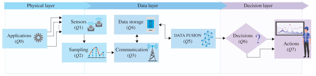
Figure 10.1 Illustration of the three layers of CPSs and their physical deployment.
Table 10.1 Guiding questions to study and/or design CPSs.
| Q# | Topic | Related question |
|---|---|---|
| Q0 | Applications | What are the applications to be implemented and their relation to the CPS function? |
| Q1 | Sensors | What kinds of sensors will be used? How many of each can be used? Where can they be located? |
| Q2 | Samples | Which type of sampling (data acquisition) method will be used? How data are coded? |
| Q3 | Communication | Which type of communication system (access, edge and core technologies) will be used? |
| Q4 | Data storage | Where are the data from sensors stored and processed (locally, in the edge and/or in the cloud)? |
| Q5 | Data fusion | Will the data be clustered, aggregated, structured, or suppressed? How? |
| Q6 | Decisions | How will the (informative) data be used to make decisions? |
| Q7 | Actions | Are there actuators and/or human interfaces? If yes, how many and where? |
In this case, Table 10.1 is constructed by acknowledging the fact that a given CPS may support, in addition to its peculiar functions, other applications that are designed either to guarantee such a functionality or to improve its effectiveness based on measurable attributes and possible interventions. As to be discussed in the following sections, the TEP can be considered a CPS where a dedicated application to detect faults can run, and thus, actions by the responsible personnel can be taken accordingly [1, 6]. Distributed coordination of actions in demand‐side management where individual devices react to a perturbation in a physical system can also be designed as a CPS [7]; this approach of a cyber‐physical energy system will be further extended in Chapter 11 when presenting the Energy Internet [7, 8] where part of the electricity interchanges in the grid are to be virtualized as energy packets to be governed as a commons [9].
10.2 Cyber‐Physical Industrial System
In this section, the focus is on CPSs that are deployed in industrial plants in order to improve their operation. The cyber‐physical industrial system addressed here is the TEP benchmark widely used in the literature of process control engineering, where faults need to be detected and classified based on acquired data. The details of the TEP are presented next.
10.2.1 Tennessee Eastman Process
The TEP was initially proposed by researchers of the Eastman Chemical Company [6]. The idea was to provide a realistic simulation model to reflect typical challenges of process control considering nonlinear relations. The physical process is characterized by the following set of irreversible and exothermic chemical reactions:

where the process has four reactants (![]() ), two products (
), two products (![]() ), one byproduct (
), one byproduct (![]() ), and one inert (
), and one inert (![]() ), resulting in eight components. The process takes place in five units, namely reactor, condenser, vapor–liquid separator, recycling compressor, and stripper. Figure 10.2 presents a schematic depiction of the TEP.
), resulting in eight components. The process takes place in five units, namely reactor, condenser, vapor–liquid separator, recycling compressor, and stripper. Figure 10.2 presents a schematic depiction of the TEP.
The details about the process can be found in [6]. What is important here is that the proposed process has 53 observable attributes; 41 measurements of the processing variables and 12 manipulated variables. The simulations proposed by Downs and Vogel [6] include 22 datasets, one being related to the normal operation of the process and 21 related to different faults that need to be detected and classified; the faults are described in Table 10.2. Attributes are measured and recorded in a synchronous manner, but with different periods: three, six, and fifteen minutes; one manipulated variable is not recorded, though. Measurements are subject to Gaussian noise. The datasets are composed of 960 observations for each 52 recorded attributes related to the lowest granularity (i.e. 3 minutes); the attributes with a higher granularity consider the latest sampled value to fill the missing points in the time series.1 Each time series has 960 points (which is equal to ![]() so that the full data set has a size
so that the full data set has a size ![]() .
.
Figure 10.2 Process flow diagram of the TEP.
Source: Adapted from [6].
Table 10.2 Faults in the TEP.
Source: Based on [10].
| Fault | Process variable | Fault type |
|---|---|---|
| 1 | A/C feed ratio, B composition constant (Stream 4) | Step |
| 2 | B composition, A/C ratio constant (Stream 4) | Step |
| 3 | D feed temperature (Stream 2) | Step |
| 4 | Reactor cooling water inlet temperature | Step |
| 5 | Condenser cooling water inlet temperature | Step |
| 6 | A feed loss (Stream 1) | Step |
| 7 | C header pressure loss – reduce availability (Stream 4) | Step |
| 8 | A, B, C feed composition (Stream 4) | Random variation |
| 9 | D feed temperature (Stream 2) | Random variation |
| 10 | C feed temperature (Stream 4) | Random variation |
| 11 | Reactor cooling water inlet temperature | Random variation |
| 12 | Condenser cooling water inlet temperature | Random variation |
| 13 | Reaction kinetics | Slow drift |
| 14 | Reactor cooling water valve | Sticking |
| 15 | Condenser cooling water valve | Sticking |
| 16 | Unknown | Unknown |
| 17 | Unknown | Unknown |
| 18 | Unknown | Unknown |
| 19 | Unknown | Unknown |
| 20 | Unknown | Unknown |
| 21 | The valve for Stream 4 was fixed at the steady‐state position | Constant position |
10.2.2 Tennessee Eastman Process as a Cyber‐Physical System
Let us consider the TEP as a CPS following the procedure described in Chapter 7; remember that the TEP is a simulation (conceptual) model that represents a typical process of an industrial plant.
- PS (a) Structural components: connections and valves; (b) operating components: reactor, condenser, vapor–liquid separator, recycling compressor‐ and stripper; (c) flow components: reactants
 ; (d) measuring components: sensors related to the different 52 attributes; (e) computing components: data acquisition module, data storage, and data processing unit (nodes connected by dashed lines); (f) communication components: cables connecting different components, and transmission and reception modules (dashed lines). The physical system is illustrated in Figure 10.2.
 - PF Generate products
 and
and  through chemical reactions between
  .
. - C1 It is physically possible to obtain
 and
and  from chemical reactions described in Section 10.2.1.
 - C2 The process has to run without faults in the different stages. Twenty‐one possible faults are described in Table 10.2, including the reactor or condenser cooling water inlet temperature and reaction kinetics, as well as unknown issues.
- C3 For the conceptual model: a software that can simulate the TEP. For an actual realization of a TEP‐like industrial process: availability of the reactants, personnel trained, the place where the physical system is to be deployed, maintenance investments, etc.
The three‐layers of the TEP as a CPS are defined as follows.
- Physical layer: The schematic presented in Figure 10.2.
- Measuring or sensing: There are 52 attributes to be measured; the devices related to the measuring process are depicted by circles. The measures are synchronized with a granularity of three minutes, but some sensors have a larger granularity (6 or 15 minutes). The measuring is subject to Gaussian noise. Data are recorded as a numerical time series in discrete time.
- Data layer: It is not explicitly described where measured data are stored and then processed, fused, or aggregated. Consequently, the structure of awareness (SAw) cannot be defined.
- Informing: The processed data are then transmitted to a central unit that makes a decision (not presented in Figure 10.2).
- Decision layer: The decision is related to: (i) successfully detect the fault considering a given probability of a false alarm, and (ii) correctly classify the type of fault.
- Acting: No action is explicitly mentioned. Possibly, if a fault is detected, the process should be stopped by an agent
 . The structure of action (SAc) is then
  .
.
The proposed framework presented in Table 10.1 can now be applied to help in defining our design problem: How to build the data layer of the TEP? We will follow the seminal work [10] considering the fault detection problem and their respective solution. Specifically, questions 3 and 4 are not explicitly considered in the already mentioned TEP seminal works (Table 10.3). More recent contributions attempting to fill this gap study, for instance, different aspects related to industrial IoT communications, including the deployment of 5G networks [11] and the impact of missing data [12].
Table 10.3 Guiding questions for the TEP as a CPS as presented in [10].
Source: Based on [10].
| Q# | Topic | Related question |
|---|---|---|
| Q0 | Application | Detect faults. |
| Q1 | Sensors | There are 52 measuring devices. |
| Q2 | Samples | Periodic sampling with different granularities (3, 6, and 15 min); all variables are in sync (3 min). |
| Q3 | Communication | Assumed perfect without explicit definition. Open for design. |
| Q4 | Data storage | Assumed that the data of the sensors are recorded and available to be processed. Open for design. |
| Q5 | Data fusion | (i) Principal component analysis (PCA), (ii) dynamic PCA, or (iii) canonical variate analysis (CVA). |
| Q6 | Decisions | |
| Q7 | Actions | Not defined; we may assume that the process stops whenever a fault is detected. |
Fault detection requires monitoring of the process in real time, i.e. whenever new samples are acquired, they need to be transmitted and processed. Although three minutes (the lowest measuring granularity in the TEP) is a reasonably large value in the domain of communication in local data networks, and the decision procedure based on either the ![]() test or the
test or the ![]() test are not computationally complex, a suitable solution for fault detection in the TEP is a many‐to‐one topology considering wireless communication links from sensors to a gateway with computational capabilities for data processing and storage. Therefore, the proposed solution is a wireless radio access technology and edge computing keeping the fault detection process within the local (industrial) area network. Figure 10.3 illustrates this design, which is a simplified version of the proposal in [11].
test are not computationally complex, a suitable solution for fault detection in the TEP is a many‐to‐one topology considering wireless communication links from sensors to a gateway with computational capabilities for data processing and storage. Therefore, the proposed solution is a wireless radio access technology and edge computing keeping the fault detection process within the local (industrial) area network. Figure 10.3 illustrates this design, which is a simplified version of the proposal in [11].
For the fault classification, the data layer solution could be different. This type of problem is defined by complete data sets containing all time‐indexed measurements. This is such an input given to the decision algorithm to classify if: (i) a fault has occurred and, if yes, (ii) which type. More advanced techniques for fault identification and then diagnosis could also be implemented in real time, also making explicit a step of expected interventions to be taken [1]. This would also lead to different requirements for the data transmission and processing, which is the focus of Exercise 10.1.
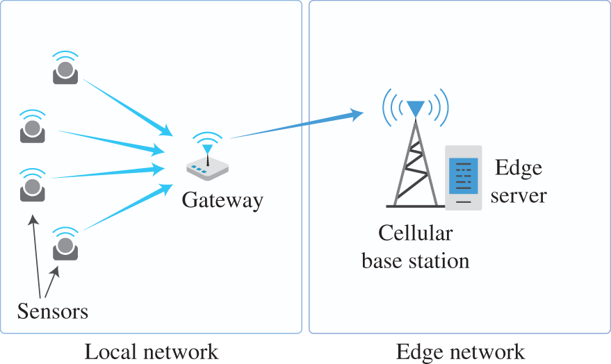
Figure 10.3 Proposed communication and storage architecture for fault detection in the TEP.
Source: Adapted from [11].
10.2.3 Example of Fault Detection in the TEP
After defining the TEP as a CPS, the attention will be devoted to exemplify the fault detection operation following the lines presented in Figure 10.1. As indicated in Chapter 9 when discussing machine learning methods, the fault detection requires a training phase where the statistical characterization of the normal process will be determined. With a full data set comprised of the time series of the 52 variables, the principal component analysis (PCA) method is used to fuse the data to reduce their dimensionality. With the reduced data set, a threshold for faults based on either the ![]() test or the
test or the ![]() test is defined considering a given level of significance that is related to an acceptable level of false alarms based on the normal operation data set. Once the threshold is defined, the fault detection can be done in real time using a rule‐based approach that considers the following: a fault happens whenever the samples associated with the current measurements are above the threshold for six times in a row.
test is defined considering a given level of significance that is related to an acceptable level of false alarms based on the normal operation data set. Once the threshold is defined, the fault detection can be done in real time using a rule‐based approach that considers the following: a fault happens whenever the samples associated with the current measurements are above the threshold for six times in a row.
Figure 10.4 illustrates the proposed fault detection in the TEP following [10]. Figure 10.4a, b present the time series of an arbitrarily chosen variable in normal operation and when Fault 5 occurs (indicated by a circle), respectively. It is visually easy to see a considerable change in the time series behavior after the fault occurs at the time index 160. However, the proposed method for fault detection consists of a statistical test based on the fused data, which include the other 51 observable attributes. Figure 10.4c, d provide a visualization of the decision process for the ![]() and
and ![]() tests, respectively. The first interesting fact is that to avoid false alarms resulting from random variations, the proposed decision rule considers subsequent states (in this case, six), and thus, the fault detection is always subject to a minimum delay (or lagging time). The second aspect is the difference between the two methods, the
tests, respectively. The first interesting fact is that to avoid false alarms resulting from random variations, the proposed decision rule considers subsequent states (in this case, six), and thus, the fault detection is always subject to a minimum delay (or lagging time). The second aspect is the difference between the two methods, the ![]() test being better than the
test being better than the ![]() to detect this specific fault because the former detects the fault in the observation 165 while the latter in the observation 173.
to detect this specific fault because the former detects the fault in the observation 165 while the latter in the observation 173.
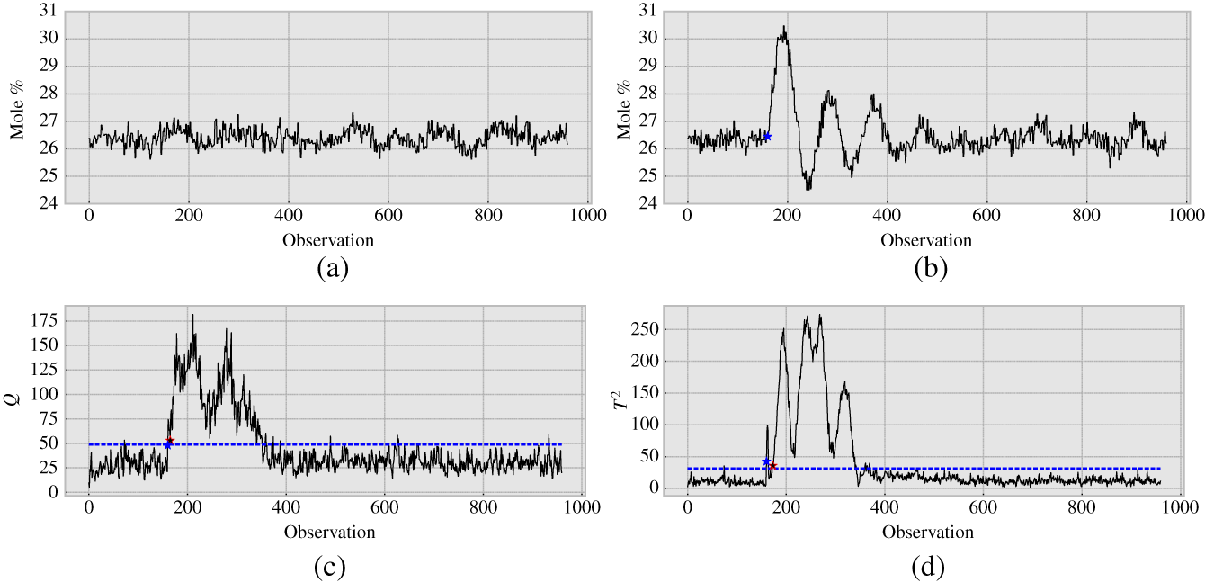
Figure 10.4 Fault detection in the TEP considering Fault 5 in Table 10.2. The first star indicates when the fault occurs. (a) Reactor feed analysis of  (stream 6): normal operation. (b) Reactor feed analysis of
  (stream 6): Fault 5. (c).
  test. The second star indicates when the fault is detected. (d)
  test. The second star indicates when the fault is detected.
This case is only a simple example of the TEP, which is still a relevant research topic for testing the performance of fault detection methods. Currently, there are several research directions that focus on different aspects, namely data acquisition (e.g. event‐triggered acquisition), advanced machine learning methods for detection, realistic models for data communications including missing samples, and data imputation for estimating missing samples to build a complete data set. Despite these advances, the most fundamental challenges of the TEP are still found in [1, 10]. The approach taken in this section provides a systematic framework to study the different opportunities of the TEP as a CPS, which includes both its aforementioned seminal results and the most recent ones as in [11, 12].
10.3 Cyber‐Physical Energy System
Energy systems are large‐scale infrastructures, whose operational management requires coordination of different elements. Specifically, modern electricity power grids are complex networks, whose operation requires a balance between supply and demand at a very low time granularity [7, 13]. This section deals with a specific intervention related to a proposal for distributed frequency control using smart fridges. Before starting this analysis, a very brief description of the power grid as a system will be provided next.
10.3.1 Electricity Power Grid as a System
The electricity power grid is an infrastructure whose main objective is to transfer energy in the electric form from one place where the electricity in generated to another where it is consumed. The grid refers to its complex physical network topology. A high‐level concept of a modern electric power grid is presented in Figure 10.5. The demarcation of the power grid as a system is proposed next.
- PS (a) Structural components: cables, towers; (b) operating components: transformers, power electronic components; (c) flow components: electric current; (e) computing components: data acquisition module, data storage, sensors, and data processing units; (f) communication components: cables connecting different components, and wireless devices.
- PF Transfer electric energy from a generating point to another consuming point.
- C1 It is physically possible to accomplish the PF.
- C2 The power transfer needs to occur so that the supply and demand are balanced. Components have to be maintained and personnel trained, and an operation center has to detect faults and react to them, etc.
- C3 Weather conditions, long‐term investments, availability of supply, existence of demand, etc.
The three‐layers of the power grid as a CPS are defined as follows.
- Physical layer: The physical components of the grid.
- Measuring or sensing: Several measuring devices for power grids to obtain the instantaneous values of, for example, current, voltage, and frequency.
- Data layer: It might be deployed at different levels: large data centers from the grid operator for near real‐time operation, cloud computing for data analysis and trends, edge computing for quick reactions, and local processing without communication.
- Informing: The communication process is usually two‐way from sensors to operators, and from operators to actuators. This depends on the level of operation that the solution is needed.
- Decision layer: This is related to decisions at different levels: it might be related to fault detection and diagnostic in the connected grid, or when to turn on a specific appliance.
- Acting: It can be from turning off a specific appliance in one household to shutting down a large part of the connected grid to avoid a blackout. This can be automated or not.
Figure 10.5 Illustration of a power grid.
10.3.2 Frequency Regulation by Smart Fridges
One of the main problems in the power grid is the frequency regulation. Alternating current power grids work synchronously with a given nominal frequency (usually 50 or 60 Hz). This means that all elements connected to the grid will experience the same frequency, which is related to the instantaneous balance between the energy supplied by the generators (mostly electric machines) that convert some form of energy into electric energy and the electric energy demanded by different loads. Then,
- if supply
 demand, then the frequency is constant;
 - if supply
 demand, then the frequency increases;
 - if supply
 demand, then the frequency decreases.
Small perturbations are allowed within a given range. When these upper and lower boundaries are crossed, the grid operation requires an intervention in order to bring the system back to its desirable state. This is usually done by adding or removing generators on the supply side.
There is also the possibility to handle this issue on the demand side, considering two facts: (i) all elements in the grid experience the same synchronized frequency, and (ii) some appliances have demand cycles that can be advanced or postponed (considering the short time frame related to frequency regulation) without affecting their function. The proposed solution is to have fridges that react to the frequency signal by postponing or advancing they cooling cycles, thereby helping to restore the frequency to its desired operation. Table 10.4 states the questions to define the design problem of these smart fridges as part of a cyber‐physical energy system.
Table 10.4 Smart fridge design in a cyber‐physical energy system.
| Q# | Topic | Related question |
|---|---|---|
| Q0 | Application | Frequency control |
| Q1 | Sensors | Observe the frequency |
| Q2 | Samples | Periodic sampling |
| Q3 | Communication | No communication |
| Q4 | Data storage | Local storage for a few samples |
| Q5 | Data fusion | No |
| Q6 | Decisions | Is the frequency within the acceptable limits? |
| Q7 | Actions | Reaction to frequency outside the limits. Open for design |
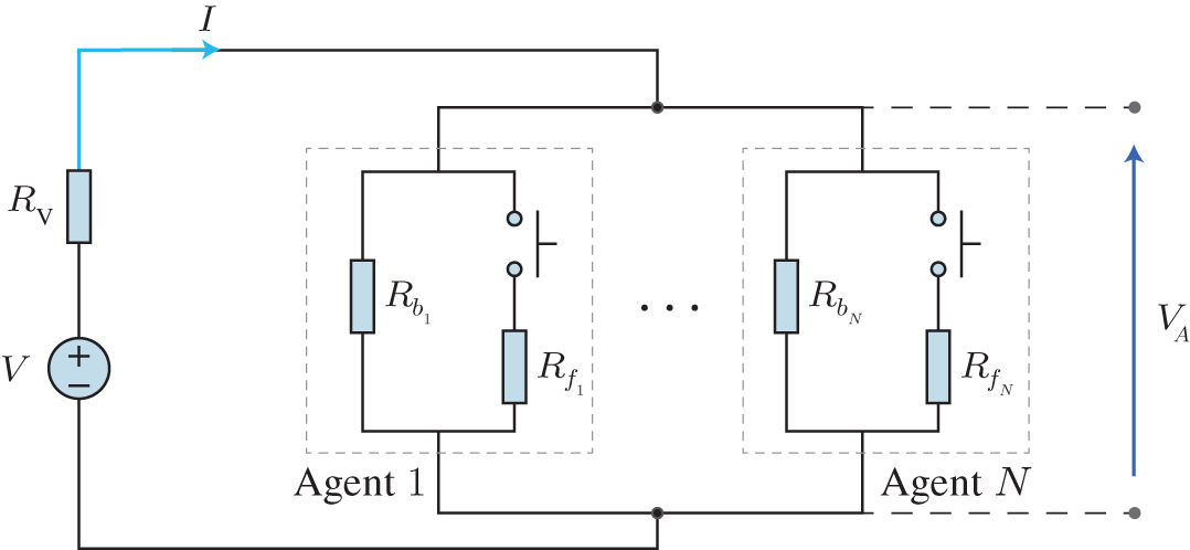
Figure 10.6 Direct current circuit representing the physical layer of the system. The circuit is composed of a power source with the voltage  and its associate resistor
  , and several resistors in parallel, controlled by
  agents. Each agent
  has a base load
  and a flexible load
  that can be used in demand‐side management. The number of active flexible loads determine the current
  .
.
Source: Adapted from [2].
To isolate the impact of different designs of actions that smart fridges could take, a simple model was proposed in [2] based on a simple direct current circuit model. Figure 10.6 presents the proposed simplified model. The rationale behind it is the following: A balanced supply (modeled as a voltage source ![]() and an associated resistor
and an associated resistor ![]() ) and demand (modeled as
) and demand (modeled as ![]() different agents representing households with a base load
different agents representing households with a base load ![]() and a flexible load
and a flexible load ![]() ) leads to a voltage
) leads to a voltage ![]() within the operational limits. This model captures the effects of adding and removing loads in AC grids, where frequency is the operational attribute to be kept within the limits
within the operational limits. This model captures the effects of adding and removing loads in AC grids, where frequency is the operational attribute to be kept within the limits ![]() and
and ![]() .
.
The dynamics of the circuit without smart fridges consists of individual fridges being on and off randomly, emulating cooling cycles. Measurements and actions are performed every second (lowest granularity). Four types of smart fridges are tested. The individual behavior of each type of smart fridge is described below.
- Smart 1: If
 , then the flexible load is off in time
  . If
. If  , then the flexible load is on in time
  . Otherwise, normal (random) behavior.
 - Smart 2: If
 , then the flexible load is off in time
  with a given probability
  . If
. If  , then the flexible load is on in time
  with a given probability
  . Otherwise, normal (random) behavior. This is similar to the ALOHA random access protocol in wireless communications.
 - Smart 3: If
 , then the flexible load will await a random time
  to check to become off so that it is off in time
  , where
  is a specific realization of the random variable
  . If
. If  , then the flexible load will await a random time
  to check to become on so that it is off in time
  , where
  is a specific realization of the random variable
  . This is similar to the CSMA random access protocol in wireless communications.
 - Smart 4: If
 , then the agent estimates from
  the numbers of fridges
  that are required to be off, and thus, the flexible load is off in time
  with a given probability
  that is a function of
  . If
. If  , then, the agent estimates from
  the numbers of fridges
  that are required to be off, and thus, the flexible load is off in time
  with a given probability
  that is a function of
  .
.
To test those different solutions, a simple numerical simulation is presented in Figure 10.7 with a setup arbitrarily chosen. The experiment consists of an intentional voltage drop between 1500 and 2000 seconds, which generates ![]() . The self‐developing dynamics of the CPS is dependent on the type of reaction assumed by the smart fridge, considering the normal case as our benchmark.
. The self‐developing dynamics of the CPS is dependent on the type of reaction assumed by the smart fridge, considering the normal case as our benchmark.
What is interesting to see is that Smart 1 and Smart 2 designs are not adaptive, and they are hard wired in a way that instead of helping, the cycles of the smart fridges become synchronized, which results in further instabilities (worse than before, because now the system swings above and below the desired operation values). Smart 4 is an improvement of Smart 2 by adapting the internal activation or deactivation probability to the estimated state of the system, considering that all other fridges are acting in the same manner. Smart 3, in its turn, offers a way to desynchronize the reactions, avoiding the harm of the undesired collective behavior. It is easy to see this by comparing the voltage behavior and the number of active flexible loads.
In this case, the SAc of the CPS is equal to ![]() , because there are
, because there are ![]() agents (
agents (![]() ) that can control their own flexible loads. What is more interesting in this study case is the SAw: (i) the benchmark scenario and Smart 1 have
) that can control their own flexible loads. What is more interesting in this study case is the SAw: (i) the benchmark scenario and Smart 1 have ![]() and (ii) Smart 2, Smart 3, and Smart 4 have
and (ii) Smart 2, Smart 3, and Smart 4 have ![]() . The difference between the strategies in (ii) is how the images of the other elements are constructed. In Smart 2 and Smart 3, the images are static, and the randomization parameters in terms of the probability
. The difference between the strategies in (ii) is how the images of the other elements are constructed. In Smart 2 and Smart 3, the images are static, and the randomization parameters in terms of the probability ![]() and time
and time ![]() and
and ![]() are fixed. Smart 4, which visually presents the best outcome, considers an adaptive randomization where all appliances will collaboratively set their
are fixed. Smart 4, which visually presents the best outcome, considers an adaptive randomization where all appliances will collaboratively set their ![]() based on an estimation of how many agents will activate their flexible load.
based on an estimation of how many agents will activate their flexible load.
It is clear that this is a very specific and controlled study case, but it serves to illustrate the importance of predicting collective behavior in systems where the same resource is shared by different autonomous agents that both (i) cannot communicate to each other and (ii) observe the same signal that guides reactions. Despite its simplicity, the model captures well a phenomenon that might occur in a future where smart appliances react to universal signals (like open market price and frequency), but act without coordination. A detailed analysis of this is found in [2].
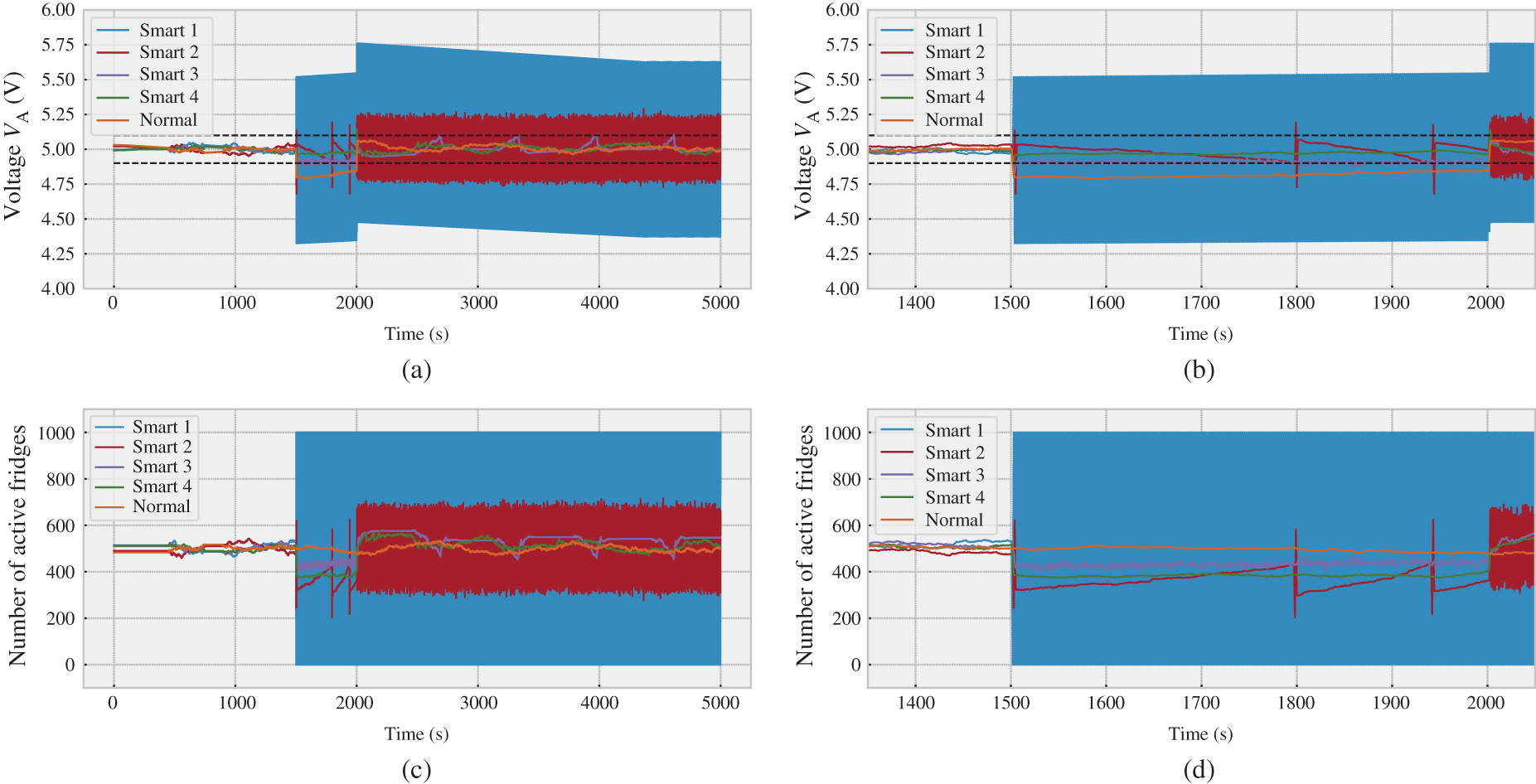
Figure 10.7 Self‐developing system dynamics considering an external perturbation. There are five scenarios, one being a baseline where the fridges are not smart and four others representing scenarios where the fridges activate their flexible load based on different decision rules. (a) Voltage observed by the agents. (b) Voltage observed by the agents zoomed in. (c) Number of active agents. (d) Number of active agents zoomed in.
10.3.3 Challenges in Demand‐Side Management in Cyber‐Physical Energy Systems
This example indicates the potential benefits of demand‐side management in cyber‐physical energy systems. However, in real‐case scenarios, the grid has a highly complex operation determined by intricate social, economical, and technical relations [14]. The main message is that, in actions related to demand‐side management, ICTs have to be used to coordinate actions by creating a dynamic estimation of the grid state at the decision‐making elements. Universal signals like the voltage in the toy example, or frequency and/or spot price in real world, may lead to undesirable collective effects that result in poor operational outcomes.
In the frequency or voltage control, the time of reaction ought to be low, and thus, the latency involved in the communication and computation might be prohibitive. In those cases, the local decision‐making process with an associated action (i.e. the decision‐maker and the agent are colocated at the same entity) as the one presented before is more suitable. This leads to a distributed decision‐making process where the decision‐making is local. Therefore, the CPS designer needs to consider that the autonomous elements are not independent, because they share the same physical infrastructure. In this case, the coordination mechanism should be internalized by the decision‐making process of the individual elements in order to mitigate the risks of undesirable collective effects.
However, at larger timescales, demand‐side management might also be related to actions associated with tertiary control with a time granularity of minutes [7]. It is at this level that the governance model assumed by the system operation is mostly felt. For example, market‐based governance models are related to individual elements aiming at maximizing profits (or minimizing costs) in a selfish manner, which may lead to systemic instabilities that result in overall higher costs despite the individually optimality of the strategy taken [15]. There are possible solutions to this problem within the market arrangements, which include direct control of loads, different price schemes, and the use of other signals like colors [14–16]. Other option is to move away from overly complex competitive market governance models (always guided by competition with myopic selfish approaches of profit maximization or cost minimization) and organize the cyber‐physical energy system as a commons to be shared, where the demand‐side management would be built upon requests, preferences, and availability [9]; the benefits of this approach will be discussed in Chapter 11.
What is important here is to indicate that cooperation among the elements that demand electric energy may use communication links and more sophisticated computing methods to coordinate their actions because the operational timescales at tertiary control allow higher latencies, compatible with decentralized or centralized ICTs. Then, the technical challenges involved here are quite different from the ones in voltage or frequency control, although the fundamental phenomenon is very similar: uncoordinated or poorly coordinated reactions that result in collective behaviors that are harmful to the CPS self‐development within its operational constraints.
10.4 Other Examples
In this section, two other cases will be presented in brief. They are: (i) a cyber‐physical solution to provide a way to record and process data related to critical public health situations like pandemics and (ii) the undesirable effects of traffic route mobile applications. These examples will be further explored in Exercises 10.3 and 10.4.
10.4.1 Cyber‐Physical Public Health Surveillance System
During the COVID‐19 pandemics, several mitigation measures were taken to prevent the virus from spreading, mainly before the availability of vaccination. Several solutions rely on explicit interventions that consider the virus propagation process based on epidemiological models over networks (see Chapter 5), whose parameters were estimated based on data collected in several ways. This type of three‐layer system is already familiar to the reader. Such a CPS is mainly designed to monitor the propagation of the virus, whose vector are humans. In this case, this would be a tool of surveillance to support public health.
As one may expect, this brings justifiable concerns in terms of privacy and reliability of the acquired data. One possible solution was proposed in [3], where the authors described a federated trustworthy system design to be implemented to support mitigation actions in future epidemics. The proposed architecture is presented in Figure 10.8, which is defined in [3] as:
A federated ubiquitous system for epidemiological warning and response. An organic and bottom‐up scaling at the global level is envisioned based on active citizens' participation. Decentralized privacy‐preserving computations are performed from the edge to the cloud based on crowd‐sourced obfuscated and anonymized data managed with distributed ledgers to empower trust. Incentive mechanisms for responsible data sharing align the public health mandate with citizens' privacy and autonomy.
The demarcation of this CPS is the task of Exercise 10.3.
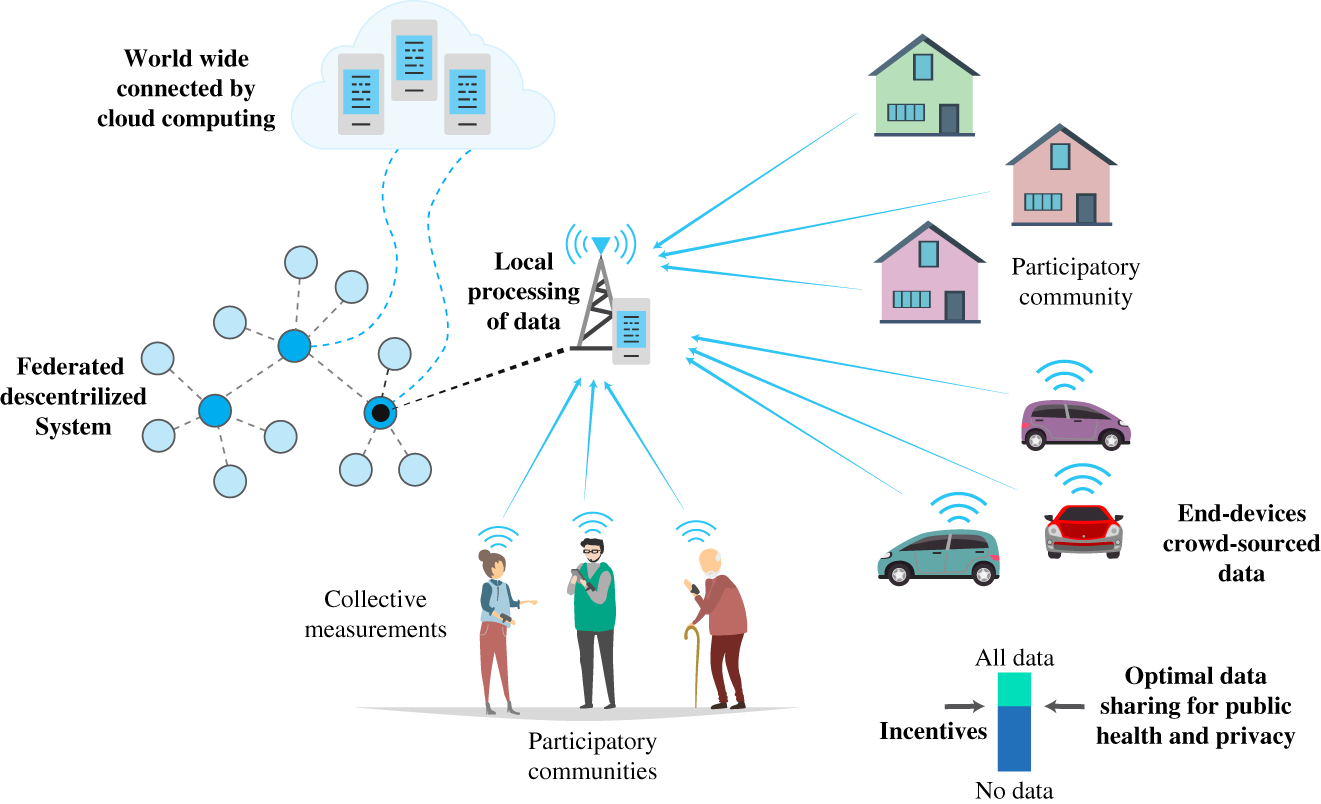
Figure 10.8 Cyber‐physical public health surveillance system.
Source: Adapted from [3].
10.4.2 Mobile Application for Real‐Time Traffic Routes
The article [4] states an undesirable problem of mobile applications designed to help drivers to select routes, usually with the aim of minimizing the travel time. In the author's own words:
Today, traffic jams are popping up unexpectedly in previously quiet neighborhoods around the country and the world. Along Adams Street, in the Boston neighborhood of Dorchester, residents complain of speeding vehicles at rush hour, many with drivers who stare down at their phones to determine their next maneuver. London shortcuts, once a secret of black‐cab drivers, are now overrun with app users. Israel was one of the first to feel the pain because Waze was founded there; it quickly caused such havoc that a resident of the Herzliya Bet neighborhood sued the company.
The problem is getting worse. City planners around the world have predicted traffic on the basis of residential density, anticipating that a certain amount of real‐time changes will be necessary in particular circumstances. To handle those changes, they have installed tools like stoplights and metering lights, embedded loop sensors, variable message signs, radio transmissions, and dial‐in messaging systems. For particularly tricky situations–an obstruction, event, or emergency–city managers sometimes dispatch a human being to direct traffic.
But now online navigation apps are in charge, and they're causing more problems than they solve. The apps are typically optimized to keep an individual driver's travel time as short as possible; they don't care whether the residential streets can absorb the traffic or whether motorists who show up in unexpected places may compromise safety.
The phenomenon described above follows a similar mechanism to Smart 1 of Section 10.3.2, where the individual decision‐making process to the signal that is broadcast to all users leads to actions that result in an undesirable collective effect. In this particular case, however, there are a few differences because not all drivers use navigation apps, and not everyone who uses them employs the same type of app. Nevertheless, the way the algorithms are designed to determine routes in real time induces several drivers to select an commonly unused path, which from time to time leads to traffic jams and other related problems of overusing and/or underusing a shared infrastructure like streets and highways.
This engineered solution for decision support can be analyzed as a CPS, where the physical layer is the traffic infrastructure including cars, the data layer is a decentralized one, where data from street and highways are acquired and then processed by cloud computing, where informative data are produced to indicate the selected route, and the decision layer is constituted by drivers, who are the final decision‐makers and agents who decide if the suggestion should be accepted and then act accordingly. It is interesting to compare how traffic jams, which are indeed unintended consequences of several cars selecting the same routes without explicit coordination, can also be formed by explicit interventions that are intended to reduce the travel time by avoiding busy routes.
Figure 10.9 illustrates this problem, described by the authors in the caption as [4]: A sporting event at a nearby stadium [A] causes a traffic backup on the highway that bypasses the center of this imaginary urban area. That's a problem for our hypothetical driver trying to get home from work, so she turns to a navigation app for help. The shortest–and, according to the app, the fastest–alternate route [dashed line] winds through a residential neighborhood with blind turns, a steep hill [B], and a drawbridge [C], which can create unexpected delays for those unfamiliar with its scheduled openings. The dotted line cuts through the city center [D] and in front of an elementary school [E]; the app doesn't know school just let out for the day. Fortunately, our driver knows the area, so she selects the full line, even though the app indicates that it isn't the fastest option. Drivers unfamiliar with the area and looking for a shortcut to the stadium could find themselves in chaotic–even hazardous–situations. A CPS designer that understands the fundamentals of collective behavior is capable of producing a solution to this problem; this is the task of Exercise 10.4.

Figure 10.9 Illustrative example of undesirable consequences of navigation apps.
Source: Adapted from [4].
10.5 Summary
This chapter presented different examples of CPSs to illustrate how the theory developed in this book is employed to study particular CPS cases. Two cases – an industrial CPS for fault detection and demand‐side management in cyber‐physical energy systems – were presented in more detail indicating positive and negative aspects that arise with the coupling between the physical and symbolic domains. Other two cases were left open for the reader as exercises. Nevertheless, the number of CPSs being currently deployed is constantly increasing, and thus, the reader can, of course, carry out a similar study considering the proposed eight questions and the demarcation based on the peculiar function with its respective necessary conditions of existence.
An important remark is that the study presented here did not focus on quantitative aspects but on qualitative ones. This decision is conscious and aims to highlight the impact of high‐level design choices in contrast to narrower mathematical results, which are heavily dependent on the specific system setting. This latter aspect is obviously of key importance and is indeed the contribution of most references used here; the reader is then invited to read them to see how the quantitative tools presented in the previous chapters are applied in those papers (although they generally do not employ the CPS conceptual apparatus developed in this book). In the next chapter, we present the still missing discussion related to aspects of CPS beyond the technology itself.
Exercises
- 10.1 Fault classification, identification, and diagnosis in the TEP. In Section 10.2.2, a communication network solution was proposed for the fault detection problem where the disturbances need to be detected regardless of their types. This question is related to the (i) classification and (ii) identification & diagnosis problems.
- Explain the difference between a fault detection presented in Section 10.2.2 and a fault classification problem considering that the full data set is already available (i.e. the classification is not real‐time).
- Based on (a), explain how the communication and storage design options change for the fault classification.
- Propose a design solution to the communication and storage considering the fault classification problem in the TEP.
- Propose a design solution to the communication and storage considering the real‐time fault identification & diagnosis problem in the TEP following the box diagram presented in Figure 10.10.
- If the process recovery intervention depends on data transmission from the decision‐maker element to possible different agents (actuators), explain the impact of this new data transmission on the data layer design.
- 10.2 Industrial CPS and energy management. The paper [17] proposes a CPS to acquire energy consumption data related to a specific industrial process. Figure 10.11 depicts the proposed solution to data acquisition of an aluminum process, including the representation of the physical, data and decision layers. The authors explain their approach as follows:
Motivated by the automatic acquisition of refined energy consumption with [Industrial] IoT technology in [mixed manufacturing system], a supply‐side energy modeling approach for three types of processes is proposed. In this approach, a data collection scheme based on sensor devices and production systems in existing software is presented, see Figure 10.11 Modules (1) and (2). Three mathematical models are developed for different energy supply modes, see Figure 10.11 Module (3). Then, the production event is constructed to establish the relationship between energy and other manufacturing elements, including job element, machine element and process element. Moreover, three mathematical models are applied to derive energy information of the multiple element dimensions, see Figure 10.11 Module (4).
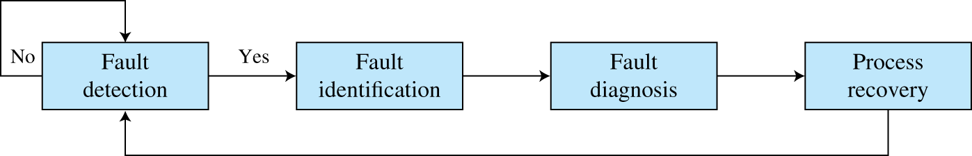
Figure 10.10 Process monitoring loop.
Source: Adapted from [1].
Without going into details of the process itself but referring to the original paper, the task of this exercise is to answer the guiding questions of this CPS presented in Table 10.5, in a similar way to the examples previously presented in this chapter.
- 10.3 CPS for public health surveillance. Read the paper [3] discussed in Section 10.4.1 and then demarcate the proposed cyber‐physical public health surveillance system employing the same approach taken in Sections 10.2.2 and 10.3.1. Refer also to Figure 10.8.
- 10.4 Suggestion of routes by mobile applications. Propose a solution to the problem described in Section 10.4.2 using the ideas presented in Sections 10.3.1 and 10.3.3.
Table 10.5 Guiding questions related to Figure 10.11.
Q# Topic Related question Q0 Application Q1 Sensors Q2 Samples Q3 Communication Q4 Data storage Q5 Data fusion Q6 Decisions Q7 Actions 
Figure 10.11 Energy data acquisition in an industrial process.
Source: Adapted from [17].
References
- 1 Chiang LH, Russell EL, Braatz RD. Fault Detection and Diagnosis in Industrial Systems. Springer; 2001.
- 2 Nardelli PHJ, Kühnlenz F. Why smart appliances may result in a stupid grid: examining the layers of the sociotechnical systems. IEEE Systems, Man, and Cybernetics Magazine. 2018;4(4):21–27.
- 3 Carrillo D, et al. Containing future epidemics with trustworthy federated systems for ubiquitous warning and response. Frontiers in Communications and Networks. 2021;2. https://www.frontiersin.org/articles/10.3389/frcmn.2021.621264/full
- 4 Macfarlane J. Your navigation app is making traffic unmanageable. IEEE Spectrum. 2019. https://spectrum.ieee.org/computing/hardware/your-navigation-app-is-making-trafficunmanageable
- 5 Gutierrez‐Rojas D, et al. Three‐layer approach to detect anomalies in industrial environments based on machine learning. In: 2020 IEEE Conference on Industrial Cyberphysical Systems (ICPS). vol. 1. IEEE; 2020. p. 250–256.
- 6 Downs JJ, Vogel EF. A plant‐wide industrial process control problem. Computers and Chemical Engineering. 1993;17(3):245–255.
- 7 Nardelli PHJ, et al. Energy internet via packetized management: enabling technologies and deployment challenges. IEEE Access. 2019;7:16909–16924.
- 8 Hussain HM, Narayanan A, Nardelli PHJ, Yang Y. What is energy internet? Concepts, technologies, and future directions. IEEE Access. 2020;8:183127–183145.
- 9 Nardelli PHJ, Hussain HM, Narayanan A, Yang Y. Virtual microgrid management via software‐defined energy network for electricity sharing: benefits and challenges. IEEE Systems, Man, and Cybernetics Magazine. 2021;7(3):10–19.
- 10 Russell EL, Chiang LH, Braatz RD. Fault detection in industrial processes using canonical variate analysis and dynamic principal component analysis. Chemometrics and Intelligent Laboratory Systems. 2000;51(1):81–93.
- 11 Hu P, Zhang J. 5G‐enabled fault detection and diagnostics: how do we achieve efficiency? IEEE Internet of Things Journal. 2020;7(4):3267–3281.
- 12 Dzaferagic M, Marchetti N, Macaluso I. Fault detection and classification in Industrial IoT in case of missing sensor data. TechRxiv. 2021.
- 13 Nardelli PHJ, Rubido N, Wang C, Baptista MS, Pomalaza‐Raez C, Cardieri P, et al. Models for the modern power grid. The European Physical Journal Special Topics. 2014;223(12):2423–2437.
- 14 Palensky P, Dietrich D. Demand side management: demand response, intelligent energy systems, and smart loads. IEEE Transactions on Industrial Informatics. 2011;7(3):381–388.
- 15 Kühnlenz F, Nardelli PHJ, Karhinen S, Svento R. Implementing flexible demand: real‐time price vs. market integration. Energy. 2018;149:550–565.
- 16 Kühnlenz F, Nardelli PHJ, Alves H. Demand control management in microgrids: the impact of different policies and communication network topologies. IEEE Systems Journal. 2018;12(4):3577–3584.
- 17 Peng C, Peng T, Liu Y, Geissdoerfer M, Evans S, Tang R. Industrial Internet of Things enabled supply‐side energy modelling for refined energy management in aluminium extrusions manufacturing. Journal of Cleaner Production. 2021;301:126882.
Note
- 1 The TEP datasets are available at https://github.com/camaramm/tennessee-eastman-profBraatz (last access: September 7, 2021).