
Step 1: Get data. That's what we have to do if we're going to build a cube.
To get data into an Analysis Services cube, we need to build a data source view (DSV). The data source view is how we represent complex relational data models for our dimension and cube design. Before we create a DSV, we'll need to create the data sources we will use to populate it. And before we do that, we'll need to create a project in BIDS.
We'll do everything I've just mentioned in this chapter, after we cover some introductory material about the data for our cube.
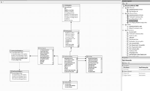
A data source view (Figure 5-1) is the layer of abstraction between a cube and the underlying data source. Although it looks like a simple ERD from a database, the important thing to note is that we're able to map tables from different data sources together into a single unified schema. Traditionally, an OLAP solution would require an OLAP-specific data store, providing the views and data structures necessary to build the cube and dimension structure. SSAS does this virtually—by building the data structure in a data source view, we can skip the step of building it physically.
In addition, by having multiple data source views, we can keep the alignment between cubes and data sources clearer. As I pointed out in Chapter 3, SSAS uses the concept of a universal data model to get away from the need for multiple data marts; using one or more data source views is part of that architecture.
You should notice something familiar about Figure 5-1: it looks like a diagram for a relational database. That's effectively what it is. We use the data source view to create a virtual schema representing relational data we can use to build our cube from. But again, because we're doing this in the Analysis Services server, we can map to tables from various servers. If we have the keys necessary to link the tables in our source systems, we can build a cube directly from those data sources—no staging database, no data warehouse, no data marts!
Mind you, in all likelihood you'll still need a staging database. The data needs to be cleaned and normalized (the key in one database is very unlikely to match to the corresponding key in another). So when you're aggregating the data, set up a staging database to act as the data source for our data source view.
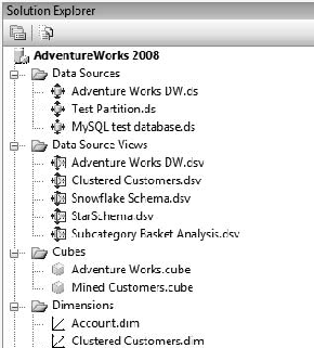
Before we can start building a data source view, we need data sources. An SSAS database can have numerous data connections (Figure 5-2), so we can have multiple data source views, and individual views can draw from multiple databases.
Data sources are pretty much as you'd expect; they capture the connection string and authentication info for a server. SSAS data sources are limited to .NET and OLE DB providers—no ODBC. When you install the provider, you'll find that the wizard just picks it up directly and it's available in the selector in the wizard (Figure 5-3).
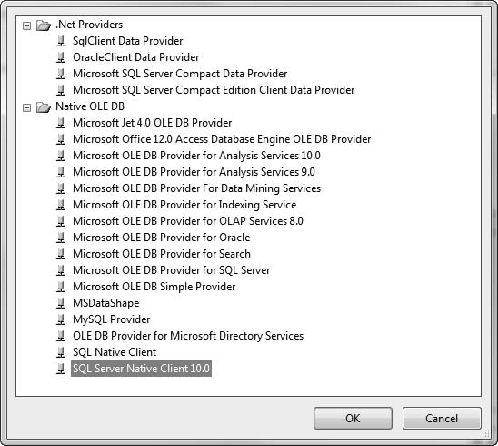
You can see in Figure 5-3 that in addition to the SQL .NET providers, there's also an Oracle .NET provider. Under OLE DB we have providers for Jet (Access), SSAS, Data Mining, DataShape (for hierarchical record sets), Oracle, MySQL, and SQL Server. Selecting a provider will load the appropriate UI for the connection information.
Creating a data source is pretty straightforward—the designer is just two panels. The first page (Figure 5-4) enables you to build the connection string with the standard Windows connection manager. The Data Source References section in the center of the page can maintain a reference to another data connection in the same project or even another SSAS project. So, for example, if you want to have two data connections with the same connection information but using different impersonation properties (to use different user accounts on a database), you could link them this way and just make changes in one location.
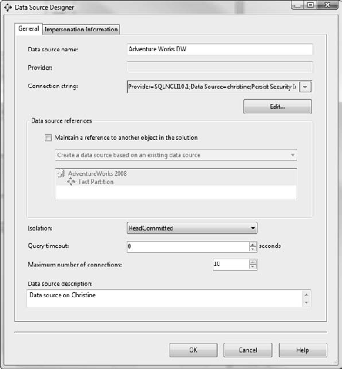
Remember that the next set of options are about an OLE DB/.NET connection, not OLAP. This is a simple data connection to a database. The Isolation level lets you enable snapshot isolation on the SQL connection, reducing row locking and contention. You can also set the timeout on the query (by default, 0 seconds means the query won't time out). Finally, you can set the maximum number of connections and a logical description.
The second tab of the designer is dedicated to the identity the connection will use when connecting. Let's look at the four options here:
- Use a specific Windows username and password:
SSAS will use the provided credentials for connecting to the data source.
- Use the service account:
The default selection, this connection will use the account information set for the Analysis Services service account. To change that account, choose Start → Administrative Tools → Services. Alternatively, press the Windows key with the R key to open the Run dialog box, and then type services.msc and press Enter. Select the SQL Server Analysis Services service, right-click and select Properties, and then select the Log On tab.
- Use the credentials of the current user:
Analysis Services will use the current user's credentials for Data Mining Extensions (DMX) queries, local cubes, and mining models. However, this option isn't valid for any action that interacts with actions that may have to cross machine boundaries—processing, ROLAP queries, linked objects, remote partitions, and synchronization from target to source.
- Inherit:
This option will pass through the credentials of the user accessing the cube or data-mining model. (See the following sidebar, "That Old Double-Hop Problem.")
Our first exercise will be a short one—let's set up a data source for the AdventureWorks DW database (see Appendix A to set up AdventureWorks). Follow the steps in Exercise 5-1.
Create a Data Source
In this exercise, you'll create a data source that you'll eventually use to build a cube. Here are the steps to follow:
Open BIDS (choose Start → All Programs → Microsoft SQL Server 2008 → SQL Server Business Intelligence Development Studio). Alternatively, you can open Visual Studio 2008 if you have that installed—you'll end up in the same place.
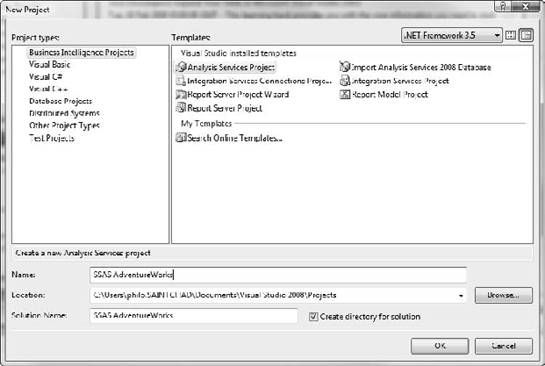
Create a new project (File → New → Project). This opens the New Project dialog box, shown in Figure 5-5.
Select Analysis Services Project, name it SSAS AdventureWorks, and click the OK button.
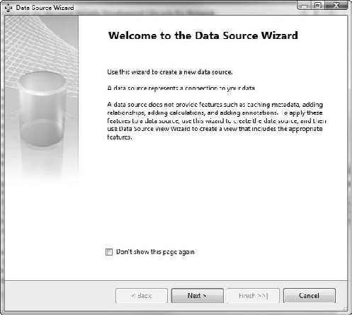
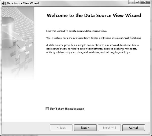
In the Solution Explorer (which is at the top right by default, or press Ctrl+Alt+L, or under the View menu if you don't see it), right-click the Data Sources folder. Click New Data Source to open the Data Source Wizard (Figure 5-6).
Click the Next button.
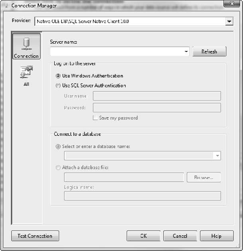
On the Select How to Define the Connection page, click the New button to create a new connection.
In the Connection Manager (Figure 5-7), ensure that the Native OLE DBSQL Server Native Client 10.0 option is selected as the provider.
For the server name, enter the name of the server where the AdventureWorks DW database is located. Note that you can use localhost here if the database is on the same machine, but be wary—you will be deploying the cube to SSAS, and the server name has to resolve there as well.
After you enter the server name, the Connect to a Database option will be enabled. Select AdventureWorksDW2008.
Click the OK button to close the Connection Manager.
Ensure that your new connection is selected in the Data Source Wizard, and then click the Next button.
Select Use the Service Account for the Impersonation Information page. (Note that the SSAS Service Account will have to have permissions to access the AdventureWorks database in SQL Server—see the sidebar "That Old Double-Hop Problem" earlier.)
Click the Next button.
On the final page, note the data source name and then click the Finish button.
Now that we have a data source, we'll need a data source view on which to build our dimensions and cubes. As I've mentioned before, you can build a data source view from multiple data sources. Simply create the additional data sources in the same manner.
The data source view defines the relational schema on which you build your cubes (consisting of measures and dimensions). As an abstraction point between an underlying database schema and the cube, the DSV allows the joining of tables that do not have relationships defined in the database, creation of primary keys on tables, calculated fields, and named queries to act as a view on data.
For the most part, the DSV is about building this relational model. If you've used a relational modeling tool in the past, it should be pretty familiar. We'll take a quick tour and then create a data source view for our cube.
As I mentioned, the DSV designer is similar to any relational model designer—add tables and link them. If you add tables that already have relationships in the underlying data source, those relationships will be shown in the DSV. You can also add relationships in the DSV, but this is to inform links; it won't create any actual constraints on the tables.
The DSV designer is shown in Figure 5-8. The central pane is the actual design surface, as you can see from the tables and relationships shown there. To the top left is the Diagram Organizer. When you get large, complex relational structures in your data source view, you can create additional diagrams to focus on subsets of the tables. The AdventureWorks SSAS solution has several functional subviews.
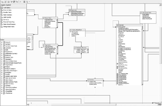
To the lower left of the designer is a table browser. You can use this for reference or drag tables from the browser to the design surface. You can also check the properties of fields by right-clicking on a field and selecting Properties. BIDS also enables viewing the data in the table: right-click on the table and select Browse Data.
If you do have a large, complex diagram and frequently need to move around looking for various tables, there are a few easy navigation methods. First and easiest—if you click on a table name in the tables pane, the diagram will immediately show that table if it's in the view. You can also click the Find Table button
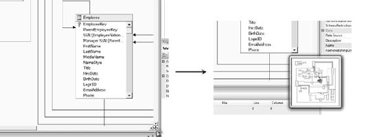
The other (really cool) way to navigate a large diagram when you're zoomed in is via the arrow in the lower-right corner of the DSV designer. When you click on the arrow, you'll see an overview of the data source view with an outline of the current view you can move to change the view (Figure 5-9).
You may need to replace a table in a data source view—perhaps with a view that has other information, or a table from another data source. If you right-click on a table, there's an option to replace the table with another table or a named query.
Warning
If you replace the table with another table that is significantly different, you stand a good chance of corrupting any dimensions or cubes that are based on that table.
Now let's take a look at creating a data source view, in Exercise 5-2.
Create a Data Source View
In this exercise, you'll build the data source view we're going to use for the rest of the book. Follow the steps in the Business Intelligence Development Studio.
Open the project from Exercise 5-1.
In the Solution Explorer in the top right, right-click on Data Source Views and select New Data Source View to open the Data Source View Wizard (Figure 5-10).
Click the Next button.
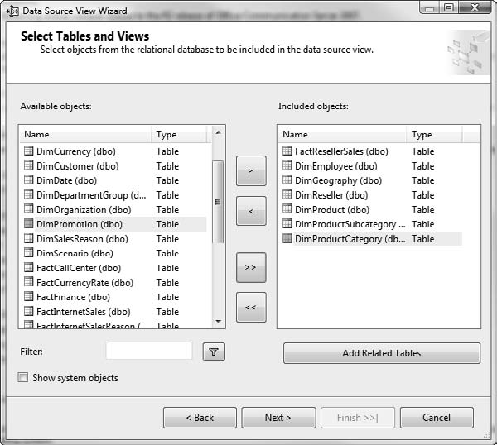
Select the data source you created, and then click the Next button to proceed to the Select Tables and Views page (Figure 5-11).
Add the tables listed in Table 5-1 by selecting them and clicking the single right-arrow (>) button.
Click the Next button.
The final page enables you to give the dat source view a name. Leave the default name and click Finish.
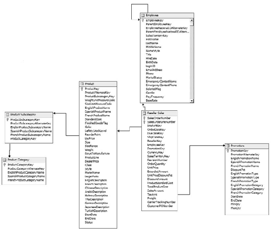
The DSV designer should open—you should see the tables with their relationships shown. Figure 5-12 shows an arrangement; yours may be somewhat different.
You can rearrange the tables to a more logical layout if you choose.
Let's give the tables more user-friendly names. Right-click on the FactResellerSales table and click Properties.
In the Friendly Name field, type Reseller Sales.
Add friendly names to each of the other tables in the same way.
Save the project. Now let's move on to named calculations and queries.
Occasionally you may need a column that can be derived from existing values, or a single table composed of columns from other tables. You can accomplish these in the data source view with named calculations and queries.
For example, invoice line item data often doesn't include the subtotal; business systems calculate it on the fly. We could calculate it in the cube, as you'll see in Chapter 7, but for something that's relatively fixed (such as a subtotal value), why not calculate it at the data source and not waste processing power recalculating it over and over?
Analysis Services lets you calculate a value in the data source view by creating a named calculation. We effectively define a dynamic field in the table in the data source view that does the math when the data is read. Using this, we can create concatenated fields (full name consisting of first name plus last name), adjusted values (age from date of birth, aligning date/time values to join tables), or various calculated values.
Named calculations are defined in the data source view. You can create a named calculation by right-clicking on a table in the designer and selecting New Named Calculation. This will open the Named Calculation dialog box (Figure 5-13). It's pretty straightforward—name and description, and the expression for the calculation.
Note
The calculation must be a standard SQL expression that returns a scalar value.
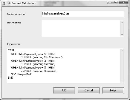
In our data source view, we have a table for Employees. The table has a start date and end date, but perhaps we want to know the number of years the employees have been on the job. For employees still in the position, the end date is null, so we'll have to use today's date. If we're looking for the number of years, we can create a named calculation, which will recalculate whenever we process the dimension. So let's look at how we create the named calculation in Exercise 5-3.
Create a Named Calculation
In this exercise, you're going to create a calculated field to show the number of years an employee has been in a role, using the start date and end date fields. If the end date field is null, you'll use today's date.
Open the SSAS AdventureWorks project again if you don't have it open.
Open the
Adventure Works DW2008.dsvdata source view.Right-click on the Employee table and select New Named Calculation.
For column name, enter YearsInRole.
In the Expression field, enter the following:
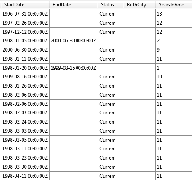
CASE
   WHEN EndDate IS NULL
      THEN DATEDIFF(year, StartDate, GETDATE())
   ELSE
      DATEDIFF(year, StartDate, EndDate)
END
Click the OK button. You'll see the new field in the Employee table.
To see the results, right-click on the table and click Explore Data. The new column will be at the end. See Figure 5-14 to see some of the data.
Save all open files.
The counterpart of a named calculation is a named query. This is effectively a SQL view as part of the data source view. The named query designer (Figure 5-15) will look very familiar to anyone who has designed a query in Access, SQL Server Management Studio, Reporting Services, and so on.
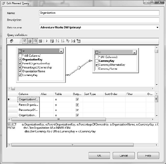
One of the top uses of a named query is to make data more readable. As shown in Figure 5-15, we want to show a label in the table instead of a numeric foreign key. Another use would be to merge tables for use in a star schema. Although a normalized database would have separate tables for county, state, and country, in our star schema we want a single table listing counties and indicating the state and country value for each. (You'll learn how to break this back down in Chapter 7.) After you create a named query, it will appear to subsequent wizards just as another table.
Let's add the Reseller table to our data source view, and include the geographic information about the reseller. Follow along in Exercise 5-4.
Create a Named Query
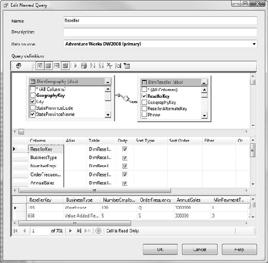
In this exercise, you'll create a named query to represent our resellers, pulling some of their geographic information into the table (instead of bringing in the whole geography set of tables).
Right-click on the design surface and select New Named Query.
Name the query Reseller.
Right-click in the table area under Query Definition and then click Add Table.
In the Add Table dialog box, select DimReseller and DimGeography and then click Add.
Note that the tables are already connected. Select the fields listed in Table 5-2 by selecting the check box next to each field name.
Table 5.2. Adding Fields to the Named Query
Table
Field
DimReseller
ResellerKey
DimReseller
BusinessType
DimReseller
NumberEmployees
DimReseller
OrderFrequency
DimReseller
AnnualSales
DimReseller
MinPaymentType
DimReseller
MinPaymentAmount
DimReseller
YearOpened
DimGeography
City
DimGeography
StateProvinceName
DimGeography
EnglishCountryRegionName
DimGeography
PostalCode
You can click the Run button to see the query results and ensure that the query is okay. The result should look like Figure 5-16.
Click the OK button.
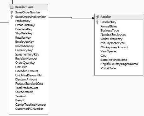
Note that in this case our Reseller view still needs to be connected to the Reseller Sales table.
First create a logical primary key on the view: right-click on ResellerKey and select Set Logical Primary Key. This marks this field as the primary key for the view.
Click and drag the field ResellerKey from Reseller Sales to the ResellerKey field in the Reseller table.
Note
If you try to drag the field the other way, you will get a warning that you are setting a relationship in an unusual direction, and you will have the option to switch the relationship.
When you're finished, the two tables should look like Figure 5-17.
Save all files—we're finished with our data source view!
Now that you understand data source views, you can see how they can be used to aggregate data from multiple data sources. Also, by using multiple data source views, you can provide different ways of looking at data without actually creating different databases and duplicating the data itself. The data source view is a key concept in the universal data model, by providing a way of severing data without duplicating it. The "model" part is formed by the dimensions and measures of the cube itself. Let's move on to understanding dimensions by creating some.