
So we have a collection of dimensions, and a pile of data in our database. The question is—now what? To get value from our data and the work we've done so far, we need to assemble the dimensions into a cube. That's what we're going to do in this chapter. In addition to building a cube from our dimensions, we'll also look into calculated measures (deriving additional values from existing values), partitions (dividing data to ease management), and a deeper dive into aggregations and their design.
A cube in SQL Server Analysis Services is basically a collection of dimensions and measures (and some metadata.) Dimensions must be defined in the database before they can be used in the cube (which is why we did them first!). After we have a collection of dimensions, we can fill in the cube with fact data. After we have our fact data loaded, Analysis Services aggregates the data in accordance with the hierarchies in the dimensions.
Let's take a look at our "spreadsheet cube" from Chapter 2, shown again here in Figure 7-1. We have three dimensions shown: Product, Country, and Order Date. At various intersections we see dollar figures representing the sales corresponding to the dimension member values. For example, in 1997, $780 worth of Alice mutton was sold in Italy. Note that the numbers we're seeing most likely aren't the leaf-level values—they were probably aggregated from individual sales records.
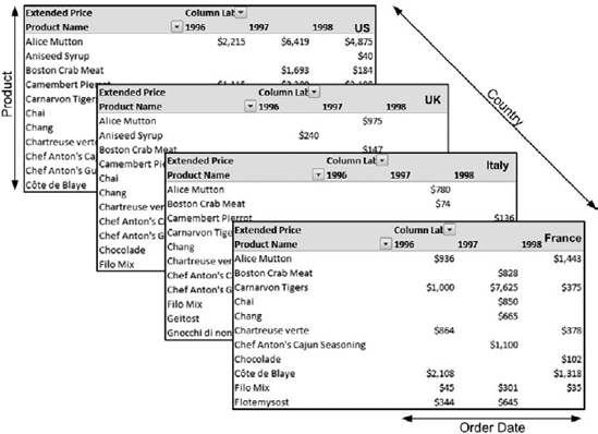
For example, that $780 worth of Alice mutton may have been 30 orders at $26 each—we have no way of knowing from this representation of the cube. When you drill all the way down to the lowest member of each dimension, you're looking at the leaf-level values, which should be representative of the actual fact data the measures are built on.
Measures are fact data that's been combined in some way. This is the reason we're building cubes in the first place. Remember that the goal of OLAP is not to inspect rows and rows of individual records, but to review aggregated data. In this case, we don't want to see a list of 30 orders that each include Alice mutton; we want to know that $780 total was ordered from Italy in 1997. To get those totals, we want the data to be aggregated in some way. SSAS allows you to define how numeric data is aggregated in a number of ways (sum, count, maximum value, average, and so forth). By default, fact data will be summed, but a cube designer can select other methods of combining values.
In addition to actual numeric data, we often want values that are derived from existing numbers. For example, very often purchase orders will have the quantity ordered and the unit cost, but won't contain the extended price (total cost for the number of items ordered).
Another aspect to aggregations is choosing how much to calculate in advance. Consider a cube with dimensions for dates, a catalog of 5,000 products, 3,140 counties (or county equivalents—I'm looking at you, Louisiana and Alaska), and 15,000 customers. At the lowest level, there are 85,957,500,000,000 unique combinations...per year! We don't want Analysis Services calculating the totals for every single combination all the way up every hierarchy. The Aggregation Designer in BIDS lets us guide Analysis Services as to how much to calculate in advance, with the remainder being figured out on the fly when a user makes a query.
We'll cover all these aspects of cubes in this chapter. Let's start with dimensions and how to build a cube.
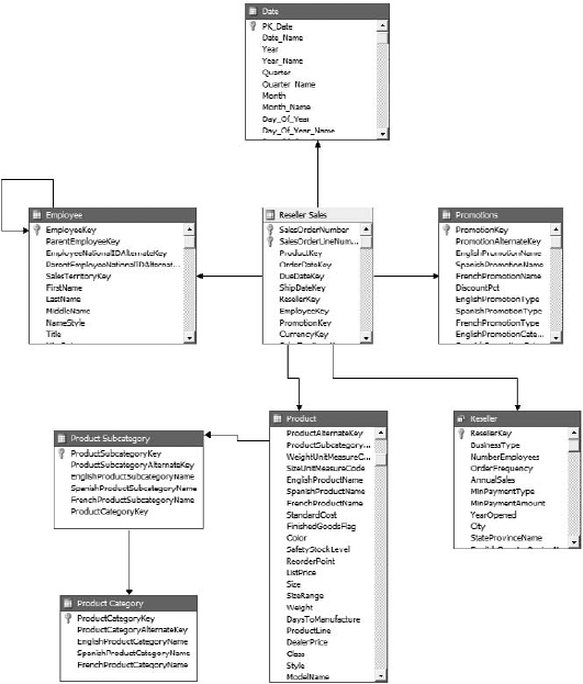
In Chapter 6, we created three dimensions: Promotions, Product, and Date. All of these are linked to the Reseller Sales table in the data source view, as shown in Figure 7-2 (with some tables excluded for clarity). The Reseller Sales table is going to be our fact table, the table containing all the detailed records we're interested in aggregating together. Product, Promotions, and Date are all dimension tables, effectively lookup tables for the ways we want to roll the reseller sales data together.
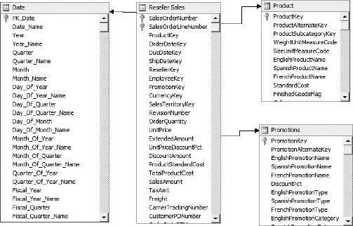
The fields in our fact table consist of a primary key (SalesOrderNumber and SalesOrderLineNumber as a composite key), a collection of foreign keys, and our line-item detail data, most of which is numeric. When we build our cube, we'll create measures out of the numeric fields. Let's take a look at the mechanics of creating a cube.
Note
Remember that measures will always be numeric. Even when you might want a measure similar to Return Reasons, what you'll really have is a dimension for the text of the reasons, and each measure value will be a count that's summed up. You'll look at this later in the chapter.
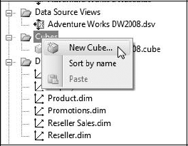
Creating a cube in BIDS is as simple as right-clicking on the Cubes folder in the Solution Explorer and selecting New Cube, as shown in Figure 7-3. This starts the Cube Wizard, which will walk you through the steps to create a new cube in the current database or database solution.
When you start the wizard, you have three options for creating a new cube:
- Use existing tables:
This is the option you'll use most often, especially when you're starting out. This wizard will walk through selecting existing dimensions, generating new dimensions from existing tables, and creating measures from fact tables. We'll use this wizard in Exercise 7-1.
- Create an empty cube:
As indicated, this option simply creates a container. You can choose to bind it to a data source view or not. For more experienced administrators, you may end up using this option more often, as you use it to simply create a cube, and then add dimensions and measures manually. This is also the best choice if you have a cube for which all the dimensions are linked dimensions.
- Generate tables in the data source:
This wizard will walk you through creating skeleton dimensions and measures. When you finish the wizard, you'll have the option to generate the schema—creating the matching tables in a data source. This is a good way to start if you know what you want the cube to look like, and have to pull data together from multiple data sources. Design the cube, and use the wizard to create a matching staging database. Then you can design SSIS transformations to load data from the data sources into the staging database.
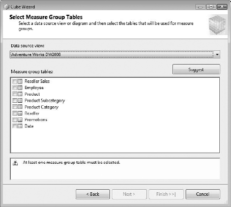
If you're creating a cube from existing tables, the next step is to select the tables that contain measures. This page of the wizard is shown in Figure 7-4. Generally, you're interested only in tables that contain fact data—the numbers and details of the transactions you're trying to track. However, you might also want measures based on data in dimension tables. For example, our Product table has a field for Standard Cost. We may want to use that in some analysis on our data later, perhaps as part of a profit margin calculation. In that case, we would include the Product table as a measure group table so we could include the StandardCost field as a measure.
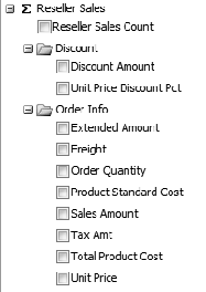
Also note the Suggest button—if you click this, BIDS will analyze the tables in the current data source view and suggest the tables that are likely to contain fact data of interest. After you've selected the tables you want to build measures from, the next page of the wizard presents the fields in those tables that are numeric. You can then select the fields you want to build measures from, as shown in Figure 7-5.
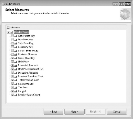
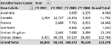
Generally, the list of proposed measures will be overinclusive, especially because foreign keys are often numeric. Deselect any fields you don't want aggregated as measures—foreign keys, counters, document numbers, and so on. Note the last field in the list, Reseller Sales Count. The wizard always adds a measure that is simply a count of the number of records. Essentially this is a field whose value is 1 in every record. When you slice a cube by dimensions, the ones will be added for each record, giving a count of the number of sales corresponding with the selection. Figure 7-6 shows a breakdown of reseller sales by country and year for AdventureWorks.
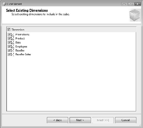
The next step in the wizard is to select the dimensions in the solution that already exist, as shown in Figure 7-7. (Linked dimensions won't be displayed.) All the dimensions will be selected by default; you just need to deselect the dimensions you don't want included in the cube. After you've selected the dimensions, the final wizard page will confirm your configuration and then create the cube.
When the wizard creates the cube, these dimensions will be included and the wizard will create associations for them with a "best guess" as to the type of association (see "Defining Dimension Usage" later in this chapter for more information). In Exercise 7-1, you'll use the Cube Wizard to create a cube for analyzing reseller sales data by using the dimensions we built in Chapter 6.
Create a Cube
In this exercise, you're going to take the dimensions you created in Chapter 6 and use them to create a cube based on the data you have in the AdventureWorks relational database.
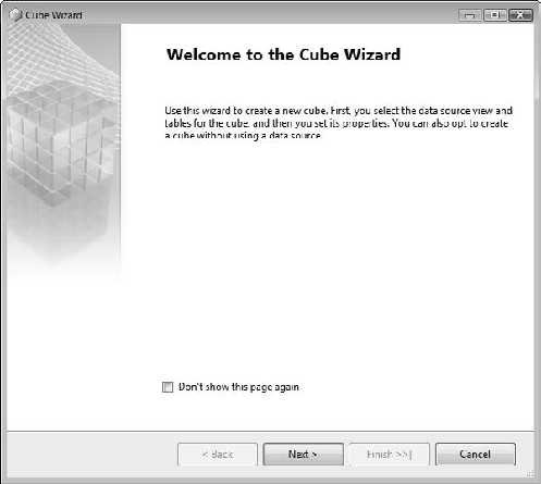
In the Solution Explorer (press Ctrl+Alt+L if it's not showing), right-click on the Cubes folder and select New Cube. This starts the Cube Wizard (see Figure 7-8).
Click the Next button.
On the Select Creation Method page, leave the default Use Existing Tables selected and click the Next button.
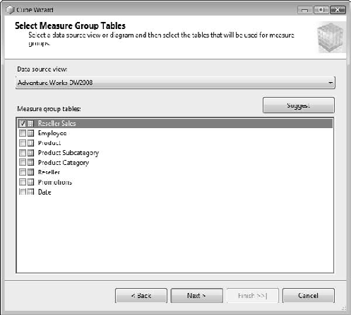
In the Select Measure Group Tables page, ensure that Adventure Works DW2008 is selected as the data source view (it should be, unless you've created another one on your own), and select Reseller Sales as the measure group table, as shown in Figure 7-9.
Click the Next button.
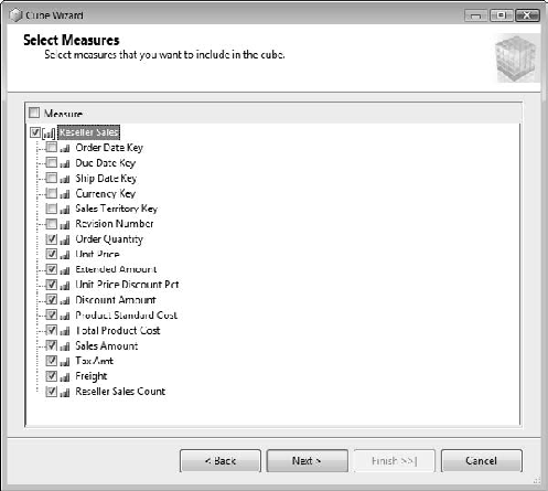
In the Select Measures page, all the fields will be selected by default: Deselect Order Date Key, Due Date Key, Ship Date Key, Currency Key, Sales Territory Key, and Revision Number, as shown in Figure 7-10.
Click the Next button.
On the Select Existing Dimensions page, ensure that Promotions, Date, and Product are selected, and then click the Next button.
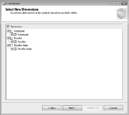
On the Select New Dimensions page, leave all three dimensions and their hierarchies selected, as shown in Figure 7-11. Click the Next button.
On the Completing the Wizard page, review the cube and click Finish. You should end up with a cube similar to what's shown in Figure 7-12. We'll use this to continue our discussion on cubes.
Save the solution.
Now that we have a cube, we know that we have a collection of fact data as measures, derived from the fields in the Reseller Sales table, and a number of dimensions. However, how does Analysis Services know how the measures and dimensions are related? We've seen some very complex schemas with dimensions related to fact tables through other dimensions, dimensions not related to fact tables, many-to-many dimensions, and so on. How does SSAS keep all this straight? Let's take a look at setting dimension usage.
In our newly created cube, let's look at the Dimension Usage tab. Each dimension is assigned a relationship to each measure group in the cube. The usage for the cube we just created is shown in Figure 7-13. Each dimension is listed, linked to the Reseller Sales measure group that was created by the wizard.
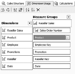
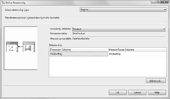
If you click the [-] button on a relationship, such as the Product relationship highlighted in Figure 7-13, you'll be presented with options for the relationship, as shown in Figure 7-14. The top section enables you to select the type of relationship between the dimension and the measure group; the lower section will change depending on the type of relationship selected.
The options available for relationship type are as follows:
- No Relationship:
There's no relationship between the dimension and the measure group. This is useful when you have many dimensions and many measure groups in a single cube, as in the AdventureWorks reference cube. Obviously, if there's no relationship, there won't be any settings to change.
- Regular:
This is a standard one-to-many reference relationship with a foreign key in the measure group and a primary key in the dimension. If you select this relationship type, you'll have to choose the attribute from the dimension that defines how the measure group is linked to it. (For example, perhaps we have a measure group regarding overhead costs for product categories; then in the Product dimension, you would select the Category granularity attribute.)
Note
If you select a dimension attribute other than the key for the granularity attribute, you must make sure all the other attributes in the dimension are also related to your key so that the server can aggregate data properly.
- Fact:
This indicates that the dimension was created from the fact table it's related to. There are no settings here to change.
- Referenced:
A referenced relationship indicates an indirect relationship through another table. For example, if we created an explicit dimension for product subcategories and related that dimension to reseller sales, we would have to indicate the indirect relationship through the Products table.
- Many-to-Many:
If we wanted to define a relationship between customers and products, we would have to use a many-to-many relationship (one customer can be related to many products; one product can be related to many customers). To define the relationship, you'll need to select the intermediate measure group and then the tables necessary to make the connection.
- Data Mining:
A relationship necessary for a data-mining dimension. We'll cover this in more depth in Chapter 13.
This may all seem like a hassle, but it becomes very important to have this kind of control when we start looking at more-complex cubes, such as the AdventureWorks cube. A portion of the dimension usage table from AdventureWorks is shown in Figure 7-15. Note the dimensions that are marked as "no relation" with various measure groups. For example, the Sales Reasons group is associated with only the Sales Reason and Internet Sales Order Details dimensions.
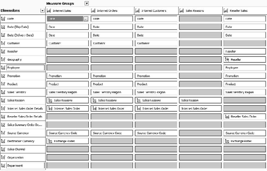
Having these measure groups and dimensions in a single place can make both development and maintenance easier, and it also provides end users an ability to combine data in a single report (for example, Internet Sales vs. Reseller Sales). If these measure groups were in separate cubes, many tools couldn't handle mapping to them both. We've talked about measure groups a lot. Let's dig more deeply into them.
We've covered the concept of measures quite a few times; measures are the numbers our users are after to analyze. They're numbers. In OLAP, they're generally aggregated in some way so that we can look at various breakdowns of values. In BIDS, you can find all the measures and measure groups in a cube on the left side of the Cube Structure tab, as shown in Figure 7-16.
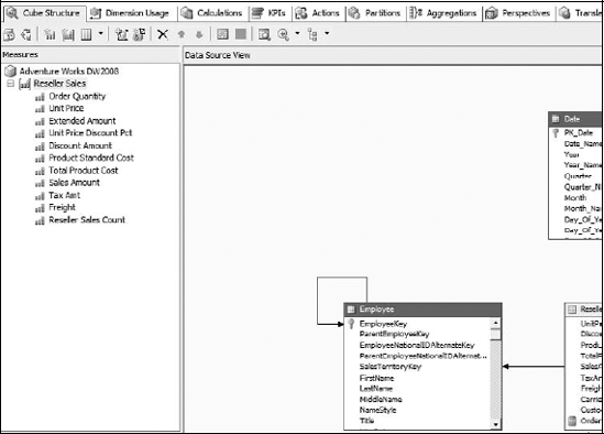
Measures are our numbers. Dimensions are around the edge; measures are in the middle, and where we're focused. Measures consist of our transactional data, and the aggregated values as we roll them up by dimension. A measure generally corresponds to a single column of data in a fact table (the table itself relates to a measure group, covered in a few pages). Take a look at Figure 7-17, showing sales data by country and territory across the top, and product categories and product lines down the left.
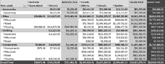
Let's say that our fact data is reported at the territory level by product line—the numbers on a white background. Those are our facts at the leaf level. They are summed by Analysis Services to produce the totals by country and by product category (gray background), and the grand totals by country and by product category (white numbers on a dark gray background). The $10 million figure in the lower right is the grand total—the summation of every fact in the cube, also the result of the (All) member on every dimension.
Native measures are generally the result of a single field; however, more-complex measures can be generated by creating a calculated measure. For example, if a record contains fields for unit cost and quantity ordered, you could have the subtotal calculated by creating a measure for unit cost x quantity. You'll take a closer look at calculated measures later in the chapter.
One of the big things we want from Analysis Services is combining numerical data. Although we generally think about simply adding the numbers together, there are other ways to combine them. Selecting a measure in the Measures pane gives us access to the properties for the measure, the first of which is AggregateFunction. The only truly additive functions (aggregated the same way along every dimension) are Sum and Count. No matter which way you slice the data, these will return the total (either adding the values or counting the records) of the child members.
There are two nonadditive aggregations: DistinctCount and None. These do not aggregate numbers. None simply performs no aggregation—if a combination of dimension members doesn't return a distinct value from the fact table, a null is returned. DistinctCount is unique in that its value must be calculated from the selection of dimension members every time—there aren't subtotals to "roll up" because distinct values may collide.
The other aggregate functions are all semiadditive; they can be aggregated along some dimensions, but not others. As mentioned previously, an inventory measure can be summed along a geographic dimension (adding inventory stock levels for different locations), but not along the Time dimension (you can't take values of 15 widgets in the warehouse in July, 20 widgets in August, and 25 widgets in September, and add them to get a result of 60 widgets—the value in September should be 25). The aggregate functions of Min/Max, ByAccount, AverageOfChildren, First/LastChild, and FirstNonEmpty are all semiadditive aggregation functions.
The DataType property is generally set to Inherited, where it will pick up the data type of the underlying measure field. You can, however, set it specifically to a data type. The data type must match the data type of the fact table field, with the exception that if the aggregate function is set to count or distinct count, the data type will reflect the integer nature of the count value.
DisplayFolder gives you a way to organize measures when you have a large number of them. This is a free-form text field. Any value you enter here will generate a folder in the measure group with the measure inside it. Folders with the same name will be combined in a measure group. See Figure 7-18 for an example.
If you need to perform a calculation to create the value of the fact data at the leaf level, you can use MDX in MeasureExpression to be evaluated before any data is aggregated. Consider a quota system in which selling widgets to customers in certain states gets an additional 10 percent bonus credit for the salesperson. To calculate the credit correctly, you have to evaluate the sale at the record (that this specific product was sold to one of those specific customers). Then the values can be added normally.
FormatString is very important . The format code you place here governs how the value is rendered by client applications (Excel, Reporting Services, and so forth). If you drop down the selector, you can see preformatted format strings for numeric values, currency, and dates. However, this is a free-form field, and you can enter any format string by using standard Microsoft formatting conventions.
That sums up the fundamentals of measures. Of course, there's more we can do with measures—we'll look at calculated measures later in the chapter, and KPIs and actions in Chapter 11. We'll dig into partitions and aggregations in Chapter 12. For now, let's take a look at how we deal with groups of measures.
A measure group is a collection of measures. (Sorry.) Specifically, they are the OLAP representation of the underlying fact table that contains the data we're reporting on. In addition, they also represent the aggregations that result from rolling up our measure data. A measure group represents all the measures from a single fact table. The measures within are based on the fields in that table or calculated view in the data source view. If you create a new measure group (in BIDS, Cube menu ® New Measure Group), you'll be asked which table to base it on. Similarly, if you create a new measure, the New Measure dialog box will prompt you for a source table and then offer the fields in that table to select from. The table you select will dictate which measure group will contain the new measure.
As you've already seen, measure groups are the containers used to associate dimensions in a cube. BIDS also uses measure groups as a starting point for partitions and aggregations. By default, partitions are set by measure group. However, they can be further divided by using a query to split the data in a measure group (for example, breaking down sales measure data by year). Aggregations are set by partition, so of course by default they'll also be set by measure group. We'll look at partitions and aggregations later in this chapter.
In general, measure groups are just containers. Let's take a look at some of the properties of a measure group and how we can use them, and then we'll dig into measures themselves. The properties for a measure group are broken down into the incredibly descriptive groups of Basic, Advanced, Configurable, Storage, and Misc. Well, let's not pay any attention to the groupings and just walk through them:
- AggregationPrefix:
This property is a leftover from the SQL Server 2000 days, when it was used to set a prefix on tables created for aggregations. It's deprecated and will probably be gone in the next version of SQL Server.
- ErrorConfiguration:
Here you can set specific responses for errors that occur when processing the cube. The configuration set here will be used as the error configuration by any new partitions created for the measure group.
- EstimatedRows:
You can enter the estimated number of rows per partition here for predictive calculations. (This number will also be used as the default on new partitions.)
- IgnoreUnrelatedDimensions:
When this is set to true, any dimensions that are not associated with the measure group will be forced to the All member when they are included in a query against the cube. For an unrelated dimension, the measure group will have the same value for every member, but forcing it back to All makes it clear to the end user what's happening.
- ProcessingMode:
Another property that's actually a default setting for new partitions. In this case, the options are Regular or LazyAggregations. The Regular setting means that data for the cube won't be available for processing until all the aggregations have been calculated. With a setting of LazyAggregations, users can query the cube after the data is loaded and before all the aggregations are complete.
- Type:
Similar to dimension types, there are several options here that help enable special business intelligence features in Analysis Services.
- StorageLocation:
This determines where the cache files for the measure group will be stored. If you click the selector button [...] you'll have a list of locations specified on the server where you can place the storage files.
- DataAggregation:
This setting dictates how data can be aggregated for the measure group.
- ProactiveCaching:
Setting up caching here will set the default proactive caching setting for any partitions created from the measure group. The dialog should look familiar from when we worked on proactive caching with dimensions in Chapter 6.
- StorageMode:
Operates the same as ProactiveCaching, explained in the preceding list item.
One final aspect to measures we want to look at are calculated measures—how we can derive values from existing values in a fact table.
Calculated measures are actually a subset of "calculated dimension members." However, we want to focus on calculated measures, because this is where you'll do most of your calculating.
We'll start by looking at the Calculations tab of the cube designer, as shown in Figure 7-19. The organizer is at the top left, calculation tools are in the lower left, and the calculation designer is the right-hand pane.
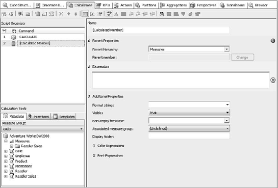
The script organizer lists all the script sections in the current cube. Script sections can be calculations, named sets, or script commands. There is one script command that is there by default, and that's the CALCULATE statement. This is the command that instructs the Analysis Services server to generate all the aggregations for the cube.
Warning
You can end up in an interesting place by accident as a result of the CALCULATE statement. If you create a new calculation and fill in a few fields, and then switch to the script view, you won't be able to switch back to the designer, because there will be a syntax error in the script as a result of the unfinished fields. You may get frustrated and just try a Ctrl+Alt+Delete. The next time you process the cube, it will run fine (no errors), but you'll have no aggregated values in your cube (the CALCULATE statement didn't run). The way to fix this is to go back to the Calculations tab and enter CALCULATE for the script command, and then reprocess.
You can create a new calculated member by choosing New Calculated Member from the Cube menu. This will create a new calculation and open the designer. The calculation will have a default name and be set to the Measures hierarchy. Note that you also have a Format string, and can set the measure group and a display folder.
The Expression box seems small, but it will automatically grow as you type. Expressions must be well-formed MDX. We'll dig into MDX in depth in Chapter 9, but we'll look at some lightweight examples here. Note that the Calculation Tools section in the lower left has the cube structure available. You can drag and drop measures, dimensions, and hierarchies from here. There's also a Functions tab, which lists all the MDX functions you may need (and then some!).
The simplest type of calculated member we've referred to previously is figuring out the total for a line item from the quantity and unit cost. This is some very simple math; we can open the Reseller Sales folder in the Metadata tab, and drag Order Quantity to the Expression box, type an asterisk (*), and then drag over Unit Price, which gives us this:
[Measures].[Order Quantity]*[Measures].[Unit Price]
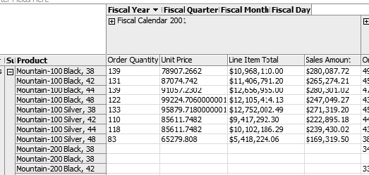
Note that BIDS inserted the parent hierarchy name ([Measures]) for us. So if we name the calculation [Line Item Total] (standard SQL syntax—you must use square brackets around item names that have spaces), and set the Format string to Currency, we can process the cube and see results similar to Figure 7-20.
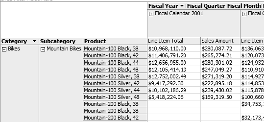
Hold on, that can't be right—why are the totals from our calculated measure so much higher than the total sales amount? Let's take a look at the order quantity and unit price, shown in Figure 7-21.
If we multiply the Order Quantity shown here by the Unit Price, we can see that it comes out to the Line Item Total. So it looks like the Line Item Total is being calculated at whatever level we're at, and that doesn't make sense for this type of calculation. (You can't multiply the total number of items bought for a period of time by the total of all the Unit Prices—remember we left Unit Price as a sum.) This value should probably be calculated as a measure expression.
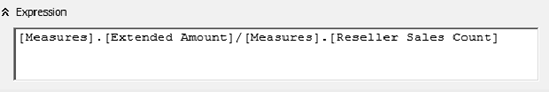
Instead, let's try calculating the average order amount per sale. We'll use this formula:
[Measures].[Extended Amount]/[Measures].[Reseller Sales Count]
This type of calculation will work well no matter what type of aggregation we have. In fact, for averages we actually want to calculate them considering all child data, no matter what level we're at. Consider two classrooms, one with 100 students, and the other with 10. The classroom with 100 students scores an average of 95 percent on an exam, while the classroom with 10 students scores a 75 percent. To figure the average score across the whole student body, you can't just average 75 percent and 95 percent to get 85 percent; you have to go back to the original data and add 110 scores together, and then divide by 110 (the answer is 93 percent).
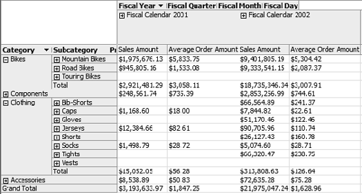
And this is a beautiful example of what makes Analysis Services so powerful. When we calculate an average based on two measures, it will produce the total of the first divided by the total of the second, based on the measures used and members selected. If we deploy, process, and check the browser, we'll see the numbers in Figure 7-22.
We can have more-complex calculations as well. This calculation in the AdventureWorks cube is as follows:
Case
    When IsEmpty( [Measures].[Reseller Sales-Sales Amount] )
    Then 0
    Else ( [Product].[Product Categories].CurrentMember,
           [Measures].[Reseller Sales-Sales Amount]) /
         ( [Product].[Product Categories].[(All)].[All],
           [Measures].[Reseller Sales-Sales Amount] )
    End
This will return for any cell associated with a product the ratio of sales for that product (or group of products) as compared to the sales for all products. You can see what this would look like in Figure 7-23. Note the CASE statement—if there is no measure from the reseller sales amount, this calculation returns a zero (for example, if you're measuring Internet sales). This highlights that calculations run against all measures in a cube, so if you're creating a calculation that is specific to a measure, you will need to exclude it from other measures.
After we're sure we're in our Reseller Sales measure, we want to calculate the sales for the currently selected group against all sales. The first half is an MDX expression indicating to use the currently selected member, while the second half indicates using all members (the grand total). Note also how the percentages don't break down across geography—only across the product hierarchy. However, every individual product, subcategory, and category is compared to the total.
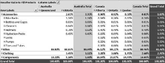
If we just wanted to see products compared to other products in their subcategory, and subcategories compared to others in their category, we could simply change the [All] to .Parent. We'll dig into MDX more in Chapter 9.
In Exercise 7-2, let's build a calculated measure just so you can be sure you know what you're doing.
Create a Calculated Measure
In this exercise, you'll create a calculated measure in our SSAS AdventureWorks cube and set some properties to take a look at how it all fits together.
Open the SSAS AdventureWorks project if you don't already have it open.
Double-click on the
Adventure Works DW2008.cubeto open it.Click the Calculations tab.
From the Cube menu, select New Calculated Member to create a new calculation and open the designer.
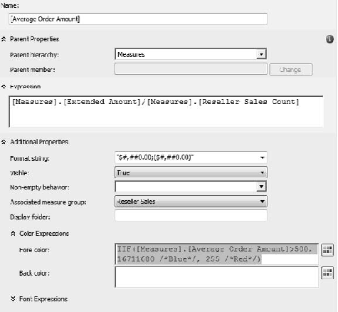
Name the calculation [Average Order Amount] (you must include the square brackets).
The Parent hierarchy should already be set to Measures.
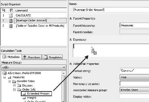
For the Expression, click the Metadata tab in the Calculation Tools section in the lower left. Open the measures, then Reseller Sales. Drag Extended Amount to the Expression window (Figure 7-24).
Type a slash (/) after
[Measures].[Extended Amount]. Then drag Reseller Sales Count over after the slash. The Expression window should look like Figure 7-25.Change the Format string to $#,##0.00;($#,##0.00).
Tip
Don't use Currency—Excel doesn't seem to recognize it.
isible should be True, and Associated Measure Group should be Reseller Sales.
Open up the Color Expressions section by clicking the two down-arrows next to the header.
Set the Fore Color text to the following:
IIF([Measures].[Average Order Amount]>500, 16711680, 255)
This translates to "If this value is greater than 500, set the text color to blue (16711680); otherwise set it to red (255)." The numbers are populated if you use the color picker button.
The final Calculation page should look like Figure 7-26.
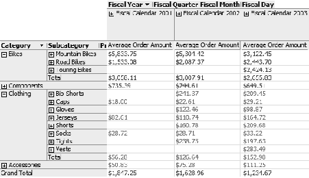
Deploy and process the cube. Then view the measure either in the BIDS browser or Excel. Both will properly render the formatting and font colors, as shown in Figure 7-27.
Save the solution.
For the most important part of our cubes, it may seem like this went more quickly than the previous chapter. As I mentioned, generally most of the work is in creating the dimensions. After that's done, generating the cube can go fairly quickly. However, we still have more work to do. Although you've deployed things a few times, you really don't have a strong grasp of what deploy and process really mean. And that's what Chapter 8 is about.