Tuples and sets are deeply connected to the problem of selecting members from dimensions. First we need to look at how we indicate which dimensions and members we're talking about. It's actually pretty straightforward—dimensions, hierarchies, attributes, and members are simply laid out in a breadcrumb manner, separated by dots.

For example, to select the LL Fork product from the Product dimension, you would use the following:

[Product].[Product].[LL Fork]

That's the Product dimension, the Product attribute hierarchy, and the LL Fork member. The square brackets are required only if the name contains numbers, spaces, or other special characters, or it's a keyword. For the preceding example, this will also work:

Product.Product.[LL Fork]

If you have a hierarchy, you will also have to specify the level from which you are selecting the member. So if you're selecting the LL Fork from the Product level of the Product Categories hierarchy, it will look like this:

[Product].[Product Categories].[Product].[LL Fork]

I do want to point out that in a hierarchy you don't "walk down" the selections. For example, note that we didn't say anything about subcategories in the preceding example. We didn't say anything about categories, either; it's just that the hierarchy is named Product Categories, so it can be a bit misleading.

Finally, we're using member names for our annotations here, mostly because they're easier to read. However, please recognize that unless you have a constraint in the underlying data source, there is no guarantee that member names will be unique. This may seem somewhat puzzling until you consider this example:

[Date].[Calendar].[Month].[November]

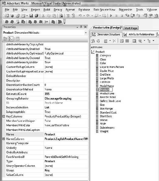
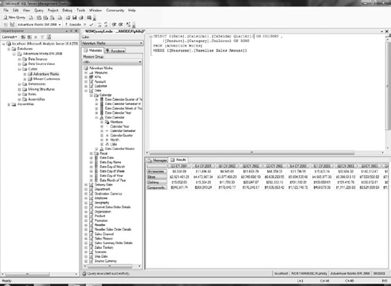
If your months are formatted in this way, that member would return an error as being ambiguous. So how do we point to that month? In MDX you also have the option of using the member key to select a member; this is indicated by prefixing the member with an ampersand. For example, LL Fork in the Product dimension will have a member key of 391. To find this member key, review the Properties pane of the Product attribute belonging to the Product dimension. The KeyColumns property lists the ProductKey field of the Product table as your member key. Figure 9-1 shows the BIDS environment with these panes displayed.

Figure 9.1. Viewing the KeyColumns property of the Product attribute

Using this value, selecting LL Fork (Product Key 391) from the AdventureWorks cube looks like this:

[Product].[Product Categories].[Product].&[391]

If you're comfortable that the member name is unique, you can replace &[391] with [LL Fork], and the query will run just fine.

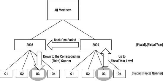
When we were building reports in the BIDS browser or Excel, we were actually building up and executing MDX queries. Let's take a look at our notional cube again, shown in Figure 9-2. We have a basic cube with three dimensions: Product, Region, and Date. Each dimension has four members. Finally, let's say the cube has a single measure: Sales Amount. Simple enough.

Figure 9.2. A cube

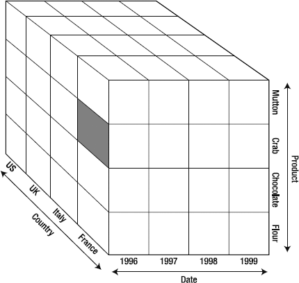
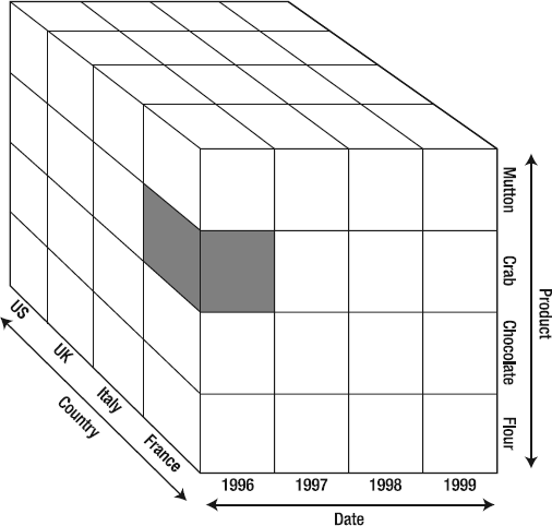
Now let's say we want to see the amount of crab sold in France in 1996. We select the appropriate members of each dimension ([Products].[Crab], [Dates].[1996], [Region].[France]), giving us the result shown in Figure 9-3. In selecting a member from each dimension in the cube, we've isolated a single cell (and therefore a single value). The highlighted area in Figure 9-3 is a tuple.

Figure 9.3. The result of selecting members of the dimensions

You may be thinking, "So a tuple is a cell?" Not quite. A tuple is the result of selecting a single member from each of the dimensions in a cube, resulting in a single cell (value) in the cube. "But wait," you say, looking at the AdventureWorks cube, "so I have to go and select a member from every single dimension every time?" Yes, but you don't have to do it by hand. Let's say you want the value of sales for all products in Italy in 1996. That would look like the cube in Figure 9-4. So—is the highlighted section a tuple?

Figure 9.4. Sales for all products in Italy in 1996

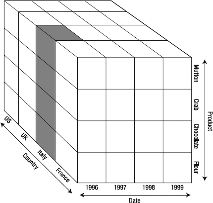
Yes! It's a tuple. "But we didn't select a member from the Products dimension," you may complain. Ah, but we did. Remember that every dimension has a default member. You can designate the default member in the Dimension Designer in BIDS for each attribute. If you don't designate a default member, Analysis Services will choose an arbitrary member from the highest level of the attribute hierarchy.

Now here's the neat part: if you indicate that an attribute can be aggregated (set IsAggregatable to true), then SSAS will automatically create a level above all the members with an (All) member, consisting of the aggregation of all members in that dimension. Because this is the top level, and has a single member, then if you don't set a default member, SSAS uses the (All) member as the default. So when we select just Italy from the notational cube, Analysis Services is providing the default member for every other dimension in the cube.

A note about annotation: tuples are always surrounded by parentheses. If you look at Figure 9-3 again, that tuple is annotated:

([Products].[Crab], [Dates].[1996], [Region].[France])

Generally, because a tuple will be a collection of members, the parentheses are pretty easy to remember. Where this will trip you up is when you use a single member to denote a tuple. For example, let's say you wanted to see the total sales for 2003. "That's easy," you would say. "The tuple would be [Date].[Calendar Year].[2003]!" No—that is the member. The tuple would be the following:

([Date].[Calendar Year].[2003])

I have a colleague whose first attempt at troubleshooting MDX queries would be to just wrap everything in parentheses. ...

Now remember that I said a tuple represents a single cell, or value, in the cube. You may look back at Figure 9-4 and say, "But there are four cells in the selection." This is true. But if you select Italy from the Region dimension and 1996 from the Date dimension, you'll get a single value—the sum of sales for all products. This often causes consternation when you're trying to design a report; you want a breakdown by product, but instead you get a single value (if you're using a bar chart, you'll get one bar, which we often call the big box, as shown in Figure 9-5).

Figure 9.5. A bar chart with one bar

So what do we do if we want to see a bar for each product? Each bar is represented by a tuple, and the four together are a set, which we'll look at in the next section.

A set is a collection of zero or more tuples. That's it. Now let's look at that bar chart again, the one with one big box. If we want the chart to show a bar for each product, we need to select the tuple for each product. The tuples for the four products are annotated like this:

{([Products].[Mutton], [Dates].[1996], [Region].[France]),
([Products].[Crab], [Dates].[1996], [Region].[France]),
([Products].[Chocolate], [Dates].[1996], [Region].[France]),
([Products].[Flour], [Dates].[1996], [Region].[France])}

This is a set—a collection of tuples with the same dimensionality. The tuples are separated by commas, and the set is set off with curly braces. Dimensionality refers to the idea that the tuples must each have the same dimensions, in the same order, and use the same hierarchy. You can use members from different levels in the same hierarchy:

{([Products].[Categories].[Category].[Bikes]),
([Products].[Categories].[Product].[Racer 150])}

But not from different hierarchies:

{([Products].[Categories].[Category].[Bikes]), ([Products].[Style].[Mens])}

You can also create a set by using the range operator (:). To do this, simply indicate the first and last members of a contiguous range, for example:

{[Date].[Calendar].[Month].[March 2002]:
[Date].[Calendar].[Month].[June 2002]}

This indicates a set consisting of four members: March 2002, April 2002, May 2002, and June 2002.

Finally, remember that a set consists of zero or more tuples, including zero and one. So yes, a tuple can be a set, or a set can contain no tuples at all (which is an empty set). This would generally be about dynamically generating sets to be used in functions. Consider the Average function, designed to return the average value of a set of tuples passed in by another function. The passing function may return a single tuple, or none for given criteria. We can either accept a set with one tuple, or we've got to write logic to read the set first and branch if the collection of tuples has only one tuple, or none. It's easier to just accept a set with a single tuple or an empty set.

Okay, hopefully you've got a loose grasp on what a tuple is, and what a set is, because we're going to start applying the concepts.

A basic MDX query consists of a SELECT statement and a FROM statement. The SELECT statement is the meat of the query; you define the axes here. This is easiest to understand with a few examples. Open SSMS (see the preceding sidebar). You can enter MDX queries and then click the Execute button to run them.

SSMS with an MDX query open is shown in Figure 9-6.

Figure 9.6. SQL Server Management Studio (SSMS) with an MDX query open

To start, let's look at a basic MDX query:

SELECT {[Measures].[Reseller Sales Amount]} ON COLUMNS ,
        {[Product].[Category]} ON ROWS
FROM [Adventure Works]

The results of this query are shown in Table 9-3. We've selected a measure member for the columns—this creates the column heading and values. Then we selected a dimension member for the rows, giving us the All Products member by default. Finally, we indicated which cube to run the query on. Note that both [Measures].[Reseller Sales Amount] and [Product].[Category] are in curly braces—the SELECT statement expects a set expression for each axis. (And even though we have just a single tuple in the first axis, a set can be a single tuple!)

What if we want a list of the product categories? The first answer is that we can simply list them, as shown in this query:

SELECT { [Measures].[Reseller Sales Amount] } ON COLUMNS ,
        {[Product].[Category].[Accessories],
        [Product].[Category].[Bikes],
        [Product].[Category].[Clothing],
        [Product].[Category].[Components]} ON ROWS
FROM [Adventure Works]

This will return the results shown in Table 9-4. This is fairly straightforward: we've selected the Reseller Sales Amount as our column (header and values), and the set consisting of each category member from the Category hierarchy in the Product dimension.

We're not restricted to a single column, either. Let's say we want to compare Reseller Sales Amount to the cost of freight. We can simply add the Reseller Freight Cost measure to the set we've selected for Columns, as shown next. This produces the result shown in Table 9-5.

SELECT { [Measures].[Reseller Sales Amount],
[Measures].[Reseller Freight Cost]} ON COLUMNS ,
        {[Product].[Category].[Accessories],
        [Product].[Category].[Bikes],
        [Product].[Category].[Clothing],
        [Product].[Category].[Components]} ON ROWS
FROM [Adventure Works]

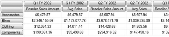
Well now we come to an interesting question: how do we use MDX to produce a pivot table? We've done a number of examples showing a breakdown of a value by one dimension in rows, and another dimension in columns. Can we show Reseller Sales Amount by Categories and Years? Sure we can—or I wouldn't have put the question in the book.

Let's try adjusting the query slightly, as shown next. The results are in Table 9-6.

SELECT { [Date].[Fiscal Year].[FY 2002],
        [Date].[Fiscal Year].[FY 2003]} ON COLUMNS ,
        {[Product].[Category].[Accessories],
        [Product].[Category].[Bikes]} ON ROWS
FROM [Adventure Works]

We see the selected fiscal years across the column headers—that's good. And we see the categories we chose as row headers—also good. But what are those dollar amounts? A little investigation would show these are the values for the Reseller Sales Amount, but where does that come from? If we check the cube properties in BIDS, we'll find that there is a property DefaultMeasure, set to Reseller Sales Amount. Well that makes sense.

But how do we show a measure other than the Reseller Sales Amount? We can't add it to either the ROWS or COLUMNS set, because measures don't have the same dimensionality as the other tuples in the set. (See how this is starting to make sense?)

What we can do is use a WHERE clause. The WHERE clause in an MDX query works just like the WHERE clause in a SQL query. It operates to restrict the query's results. In this case, we can use the WHERE clause to select what measure we want to return. So we end up with a query as shown here:

SELECT { [Date].[Fiscal Year].[FY 2002],
        [Date].[Fiscal Year].[FY 2003]} ON COLUMNS ,
        {[Product].[Category].[Accessories],
v[Product].[Category].[Bikes]} ON ROWS
FROM [Adventure Works]
WHERE ([Measures].[Reseller Freight Cost])

In addition to selecting the measure we want to look at, we can also use the WHERE clause to limit query results in other ways. The following query will show results similar to the previous one, but with the measure restricted to sales in the United States:

SELECT { [Date].[Fiscal Year].[FY 2002],
        [Date].[Fiscal Year].[FY 2003]} ON COLUMNS ,
        {[Product].[Category].[Accessories],

[Product].[Category].[Bikes]} ON ROWS
FROM [Adventure Works]
WHERE ([Measures].[Reseller Freight Cost],
        [Geography].[Country].[United States])

This use of the WHERE clause is also referred to as a slicer, because it slices the cube. When looking at an MDX query, remember that the WHERE clause is always evaluated first, followed by the remainder of the query (similar to SQL). Although these two examples seem very different (one selecting a measure, the other slicing to a specific dimension member), they're not. Measures in OLAP are just members of the [Measures] dimension. In that light, both selectors in the second query ([Reseller Freight Cost] and [United States]) are selecting a single member of their respective dimensions.

You saw how to create a grid with multiple member values. However, having to list all the members in a large hierarchy will get unwieldy very quickly. In addition, if members change, we could end up with invalidated queries. However, MDX offers functions that we can use to get what we're looking for. MDX functions work just as functions in any language: they take parameters and return an object. The return value can be a scalar value (number), a set, a tuple, or other object.

In this case, either the Members function or the Children function will work to give us what we are looking for. Let's compare the two. The following query produces the results in Table 9-7.

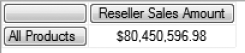
SELECT { [Measures].[Reseller Sales Amount] } ON COLUMNS ,
        {[Product].[Category].Members} ON ROWS
FROM [Adventure Works]

Now let's look at a query using the Children function, and the results shown in Table 9-8.

SELECT { [Measures].[Reseller Sales Amount] } ON COLUMNS ,
        {[Product].[Category].Children} ON ROWS
FROM [Adventure Works]

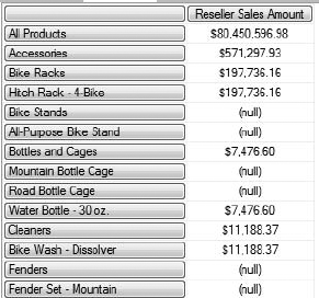
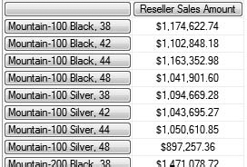
It's pretty easy to see the difference: the Members function returns the All member, while the Children function doesn't. If you try this on the [Product Categories] hierarchy, you'll see the extreme difference, because Members returns all the members from the [Categories] level, the [Subcategories] level, and the [Products] level, as shown in Figure 9-7. Note that we have All Products, then Accessories (category), then Bike Racks (subcategory), and then finally the products in that subcategory. On the other hand, Figure 9-8 shows selecting all the children under the Mountain Bikes subcategory.

Figure 9.7. Selecting a hierarchy Members collection

Figure 9.8. Selecting all the products under the Bikes category

We'll take a closer look at moving up and down hierarchies later in the chapter.

There's another difference between SQL and MDX that I haven't mentioned yet. In SQL we learn that we cannot depend on the order of the records returned; each record should be considered independent. However, in the OLAP world result sets are governed by dimensions, and our dimension members are always in a specific order. This means that concepts such as previous, next, first, and last all have meaning.

First of all, at any given time in MDX, you have a current member. As we are working with the cube and the queries, we consider that we are "in" a specific cell or tuple, and so for each dimension we have a specific member we are working with (or the default member if none are selected).

The CurrentMember function operates on a hierarchy ( [Product Categories] in this case) and returns a tuple representing the current member. If we run this, we get the result shown in Figure 9-9. Remember, a tuple is also a set.

Figure 9.9. The Reseller Sales Amount query using a CurrentMember function

For example, let's say for a given cell you want the value from the cell before it (most commonly to calculate change over time, but you may also want to produce a report of change from one tooling station to the next, or from one promotion to the next). Generally, the dimension where we have the most interest in finding the previous or next member is the Time dimension. We frequently want to compare values for a specific period to the value for the preceding period (in sales there's even a term for this—year over year growth).

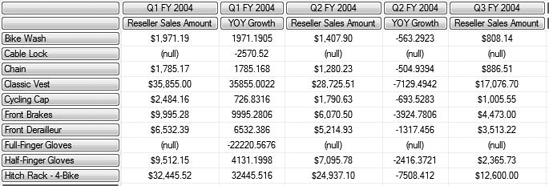
Let's look at an MDX query for year over year growth:

WITH
        MEMBER [Measures].[YOY Growth] AS
                ([Date].[Fiscal Quarter].CurrentMember,
[Measures].[Reseller Sales Amount])-
                ([Date].[Fiscal Quarter].PrevMember,
[Measures].[Reseller Sales Amount])
SELECT NONEMPTY([Date].[Fiscal Quarter].Children *
{[Measures].[Reseller Sales Amount],
[Measures].[YOY Growth]}) ON COLUMNS ,
        NONEMPTY([Product].[Model Name].Children) ON ROWS
FROM [Adventure Works]
WHERE ([Geography].[Country].[United States])

There are a number of new features we're using here. First let's look at what the results would look like in the MDX Designer in SSMS, shown in Figure 9-10.

Figure 9.10. Results of the MDX query

Well the first thing we run into is the WITH statement—what's that? In an MDX query, we use the WITH statement to define a query-scoped calculated measure. (The alternative is a session-scoped calculated measure and is defined with the CREATE MEMBER statement, which we won't cover here.) In this case, we have created a new measure, [YOY Growth], and defined it.

The definition follows the AS keyword, and creates our YOY measure as the difference between two tuples based on the [Fiscal Quarter] dimension and the [Reseller Sales Amount] measure. In the tuples, we use the CurrentMember and PrevMember functions. As you might guess, they return the current member of the hierarchy and the previous member of the hierarchy, respectively.

Look at this statement:

([Date].[Fiscal Quarter].CurrentMember,
[Measures].[Reseller Sales Amount])
-
([Date].[Fiscal Quarter].PrevMember,
[Measures].[Reseller Sales Amount])

Note the two parenthetical operators, which are identical except for the operator at the end. Each one defines a tuple based on all the current dimension members, except for the [Date] dimension, where we are taking the current or previous member of the [Fiscal Quarter] hierarchy, and the [Reseller Sales Amount] member of the [Measures] dimension.

As the calculated measure is used in the query, for each cell calculated, the Analysis Services parser determines the current member for the hierarchy, and creates the appropriate tuple to find the value of the cell. Then the previous member is found, and the value for that tuple is identified. Finally, the two values are subtracted to create the value returned for the specific cell.

Our next new feature in the query is the NONEMPTY function. Consider a query to return all the Internet sales for customers on July 1, 2001:

SELECT [Measures].[Internet Sales Amount] ON 0,
([Customer].[Customer].[Customer].MEMBERS,
    [Date].[Calendar].[Date].&[20010701]) ON 1
FROM [Adventure Works]

If you run this query, you'll get a list of all 18,485 customers, most of whom didn't buy anything on that particular day (and so will have a value of (null) in the cell). Instead, let's try using NONEMPTY in the query:

SELECT [Measures].[Internet Sales Amount] ON 0,
NONEMPTY(
    [Customer].[Customer].[Customer].MEMBERS,
    {([Date].[Calendar].[Date].&[20010701],
    [Measures].[Internet Sales Amount])}
) ON 1
FROM [Adventure Works]

The results here are shown in Table 9-9. Note that now we have just the five customers who made purchases on July 1. The way that NONEMPTY operates is to return all the tuples in a specified set that aren't empty. (Okay, that was probably obvious.) Where it becomes more powerful is when you specify two sets—then NONEMPTY will return the set of tuples from the first set that are empty based on a cross product with the second set.

Let's consider two dimensions, [Geography] and [Parts]. The [Geography] dimension has a hierarchy including [Region]. Now we want to create a report showing parts purchased by country for the countries in the North America region (Canada, Mexico, United States). If you look at the data in Figure 9-11, note that only five of the products out of eleven had sales in the countries we're interested in (shaded).

Figure 9.11. Using NONEMPTY

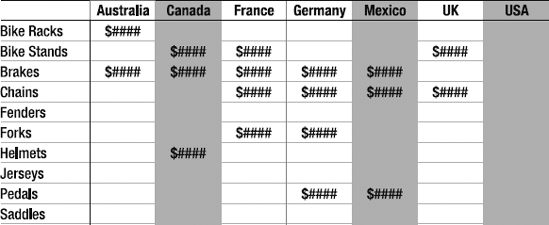
So we want to use the NONEMPTY function:

NONEMPTY(
[Parts].Members,
{
([Geography].[Region].[North America].Members, [Measures].[Sales Amount])
})

This will return the list of members of the Parts dimension that have values in the North America region for the Sales Amount measure, and will evaluate to {[Bike Stands], [Brakes], [Chains], [Helmets], [Pedals]}.

The second NONEMPTY function has just one argument:

NONEMPTY([Product].[Model Name].Children) ON ROWS

This will evaluate and return a set of members of the Model Name hierarchy that have values in the current context of the cube (taking into account default members and measures as well as the definition in the query).

Now that you know about functions, it's time to look at the different categories that are available to you. MDX offers functions relating to hierarchies, to aggregations, and to time.

Tree Functions

We've learned the importance of structure in OLAP dimensions—that's why we have hierarchies. Now we'll get into how to take advantage of those hierarchies in MDX. In SQL we learned to never presume what order records are in. If we needed a specific order, we had to ensure it in a query or view. In Analysis Services we define the order in the dimension (or there's a default order that doesn't change).

What this means is that we can operate on dimension members to find the next member or previous member. We can move up to parents or down to children. We do these with a collection of functions that operate on a member to get the appropriate "relative." For example, run the following query in SSMS:

SELECT [Measures].[Internet Sales Amount] ON 0,
[Date].[Calendar].[Month].[March 2002].Parent ON 1
FROM [Adventure Works]

This should return the Internet Sales for Q1, Calendar Year 2002, the parent of March 2002 in the Calendar hierarchy. In the preceding query, Parent is a function that operates on a member and returns the member above it in the hierarchy. If you execute Parent on the topmost member of a hierarchy, then SSAS will return a null.

You can "chain" Parent functions—for example, .Parent.Parent to get the "grandparent," or two levels up the hierarchy. But this becomes quickly painful. Instead there is the Ancestor() function to move up a dimensional hierarchy, as shown in the following query.

SELECT [Measures].[Reseller Sales Amount] ON 0,
Ancestor([Product].[Product Categories].[Product].[Chain],
    [Product].[Product Categories].[Subcategory]) ON 1
FROM [Adventure Works]

Ancestor() takes two arguments. The first is the dimension member to operate on, and the second is the hierarchy level to move up to. In the preceding query, we return the Subcategory for the [Chain] member of products. Ancestor() can also take a numeric value instead of a hierarchy level. In that case, the result returned is the specified number of steps up from the member in the first argument.

Note

The second argument for Ancestor() is the level name, not a member name.

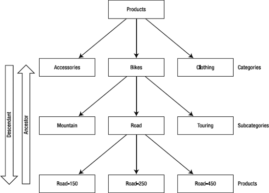
Now that we've moved up the tree from a given member, let's look at how we move down. If you think about a tree, you should quickly realize that while moving up a tree always gives us a specific member, moving down a tree is going to give us a collection of members. So it is that while the functions to move up return members, the functions to move down return sets. If you look at Figure 9-12, the ancestor of, for example, the Touring Bikes subcategory is the Bikes category (single member). The ancestor of the Road-150 product is the Road Bikes subcategory (single member). On the other hand, the descendants of the Bikes category are the Mountain Bikes, Road Bikes, and Touring Bikes subcategories (set of members).

Figure 9.12. Ancestors vs. descendants in a tree

In the same vein, analogous to the .Parent function, we have .Children. However, as you have probably figured out, while .Parent returns a member, .Children returns a set. Try the following query:

SELECT [Measures].[Reseller Sales Amount] ON 0,
([Product].[Product Categories].[Bikes].Children) ON 1
FROM [Adventure Works]

You should get a breakdown of the reseller sales by the three subcategories under Bikes (Mountain Bikes, Road Bikes, Touring Bikes).

Note

If you want to move down a hierarchy but return a single member, you can use the .FirstChild or .LastChild operators to return a single member from the next level in the hierarchy.

Aggregate Functions

One of the major reasons we've wanted to do the OLAP thing is to work with aggregated data. In all the examples you've seen to date, all the individual values are the result of adding the subordinate values (when we look at sales for Bikes in June 2003, we're adding all the individual bicycle sales for every model together for each day in June).

Let's look at an example:

WITH
    MEMBER [Measures].[Avg Sales] AS
        AVG({[Product].[Product Categories].CurrentMember.Children},
            [Measures].[Reseller Sales Amount])
SELECT
    NONEMPTY([Date].[Fiscal Quarter].Children *
    {[Measures].[Reseller Sales Amount],
    [Measures].[Avg Sales]}) ON COLUMNS ,
    NONEMPTY([Product].[Product Categories].Children) ON ROWS
FROM [Adventure Works]
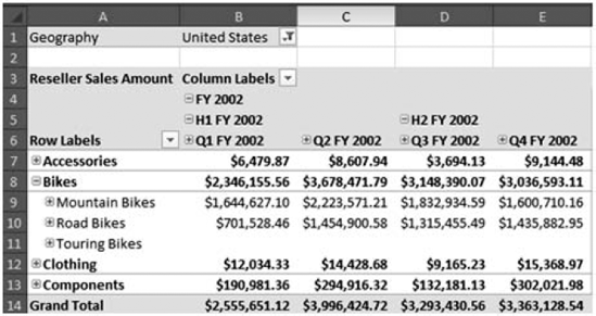
WHERE ([Geography].[Country].[United States])

In this query, we've created a calculated measure using the AVG() function, which will average the value in the second argument across the members indicated in the first argument. In this case we've used CurrentMember to indicate to use the current selected member of the Product Categories hierarchy, and then take the children of that member. In the SELECT statement, we then use the cross product between the set of fiscal quarters and the set consisting of the Reseller Sales Amount measure and our calculated measure. (This produces the output that displays the two measures for each quarter.) Part of the output is shown in Figure 9-13.

Figure 9.13. The output of the AVG() query

We can use Excel to examine the data underlying our grid here. Connect Excel to the AdventureWorks cube and create a pivot table with Categories down rows, Fiscal Quarters across the columns, and add a filter for the United States. You can then drill down into the subcategories, as shown in Figure 9-14, and do the math yourself to check the averages.

Figure 9.14. Verifying the averages from the AVG() query

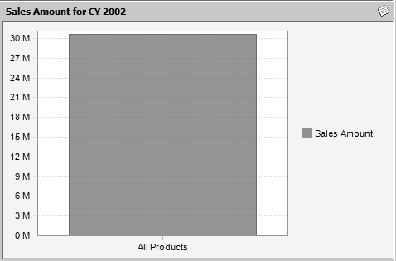
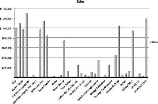
Another aggregate function that is very useful, and leverages the capabilities of SSAS well, is TOPCOUNT(). Often when you're doing analysis on business data, you'll see the 80/20 rule in action: 80 percent of your sales are in 20 percent of the regions, products, styles, and so forth. So you end up with charts that look like the one in Figure 9-15.

Figure 9.15. Sales across a range of products

What we're probably interested in is our top performers; for example, how did the top ten products sell? In T-SQL we can use a TOP function after sorting by the field we're interested in; in MDX we have TOPCOUNT().

Let's adjust our MDX query with the [Avg Sales] measure from before:

WITH
    MEMBER [Measures].[Avg Sales] AS
        AVG({[Product].[Product Categories].CurrentMember.Children},
            [Measures].[Reseller Sales Amount])
SELECT NONEMPTY([Date].[Fiscal Year].Children *
    {[Measures].[Reseller Sales Amount],
    [Measures].[Avg Sales]}) ON COLUMNS ,
    NONEMPTY([Product].[Product Categories].Subcategory.Members) ON ROWS
FROM [Adventure Works]
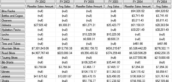
WHERE ([Geography].[Country].[United States])

First, I've changed the time dimension from fiscal quarters to fiscal years, just to make the results easier to see. Second, I've changed the SELECT statement to select Subcategory.Members from the [Product Categories] hierarchy. Note that I've changed .Children to .Members. Although the [Product Categories] hierarchy has a member named Members, the [Subcategory] level doesn't, so we use Children.

This query will return results as shown in Figure 9-16. If we just look at FY 2004, the average sales range from $462 to $362,000. In fact, more than 98 percent of our sales are concentrated in the top ten items.

Figure 9.16. Results of the Average Sales query across all subcategories

If we want to focus our business on the highest performers, we want to see just those top performers. So let's take a look at the query necessary:

WITH
    MEMBER [Measures].[Avg Sales] AS
        AVG({[Product].[Product Categories].CurrentMember.Children},
        [Measures].[Reseller Sales Amount])
SELECT
    NONEMPTY([Date].[Fiscal Year].Children *
    {[Measures].[Reseller Sales Amount],
    [Measures].[Avg Sales]}) ON COLUMNS ,
    TOPCOUNT(
        [Product].[Product Categories].Subcategory.Members,
        10,
        [Measures].[Reseller Sales Amount]) ON ROWS
FROM [Adventure Works]
WHERE ([Geography].[Country].[United States])

The only thing I've changed here is to add the TOPCOUNT() function to the rows declaration; this will return the top ten subcategories based on reseller sales. You'll notice that in several years the top sellers have a (null) for the sales amount—so why are they in the list? The trick to TOPCOUNT() is that it selects based on the set as specified for the query. In this case, we get the AdventureWorks cube sliced by the US geography, and the top subcategories are evaluated from that. After we have those top ten, those subcategories are listed by fiscal year.

Okay, now let's wrap up our tour of MDX queries with one of the main reasons we really want to use OLAP: time functions.

Time Functions

Much of the analysis we want to do in OLAP is time based. We want to see how data this month compares to the previous month, or perhaps to the same month last year (when looking at holiday sales, you want to compare December to December). Another comparison we often want to make is year to date, or YTD (if it's August, we want to compare this year's performance to the similar period last year, for example, January to August).

These queries in SQL can run from tricky to downright messy. You end up doing a lot of relative date math in the SQL language, and will probably end up doing a lot of table scans. In an OLAP solution, however, we're simply slicing the cube based on various criteria—what Analysis Services was designed to do.

So let's take a look at some of these approaches. We'll write queries to compare performance from month to month, to compare a month to the same month the year before, and to compare performance year to date.

We'll start with this query:

Select
   Nonempty([Date].[Fiscal].[Month].Members) On Columns,
   TopCount([Product].[Product Categories].Subcategory.Members,
   10,
   [Measures].[Reseller Sales Amount]) On Rows
From
   [Adventure Works]
Where
   ([Geography].[Country].[United States], [Date].[Fiscal Year].[FY 2004])

This will give us the reseller sales for the top ten product subcategories for the 12 months in fiscal 2004.

The first thing we want to look at is adding a measure for growth month to month:

WITH
    MEMBER [Measures].[Growth] AS
    ([Date].[Fiscal].CurrentMember,[Measures].[Reseller Sales Amount]) -
    ([Date].[Fiscal].PrevMember, [Measures].[Reseller Sales Amount])
SELECT NONEMPTY([Date].[Fiscal].[Month].Members
    * {[Measures].[Reseller Sales Amount], [Measures].[Growth]})
    ON COLUMNS ,
    TOPCOUNT([Product].[Product Categories].Subcategory.Members,
      10,
      [Measures].[Reseller Sales Amount])
    ON ROWS
FROM [Adventure Works]
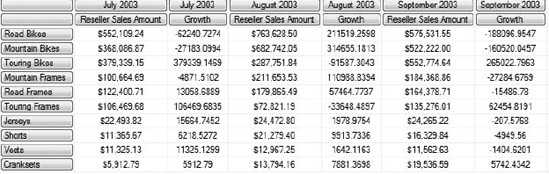
WHERE ([Geography].[Country].[United States], [Date].[Fiscal Year].&[2004])

We've added a calculated measure ([Measures].[Growth]) that uses the .CurrentMember and .PrevMember functions on the [Date].[Fiscal] hierarchy. (Note that you can't use the member functions on [Date].[Fiscal].[Month], as you may be tempted to—you can use them only on a hierarchy, not a level.) This will give us a result as shown in Figure 9-17.

Figure 9.17. Showing sales change month to month

Of course, the numbers look awful. Let's add a FORMAT() statement to our calculated measure:

WITH
    MEMBER [Measures].[Growth] AS
      Format(([Date].[Fiscal].CurrentMember,
        [Measures].[Reseller Sales Amount]) -
        ([Date].[Fiscal].PrevMember,
        [Measures].[Reseller Sales Amount]), "$#,##0.00")

Now we'll get results that look like Figure 9-18.

Figure 9.18. Formatting our calculated measure

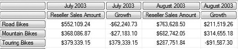
By formatting the measure in the MDX, we find that when we use any well-behaved front end, we get the same, expected, formatting.

Our bike sales are probably seasonal (mostly sold in the spring and summer, with a spike at Christmastime), so comparing month to month may not make sense. Let's take a look at comparing each month with the same month the previous year. For this, we just need to change our calculated measure as shown:

WITH
    MEMBER [Measures].[Growth] AS
      Format(([Date].[Fiscal].CurrentMember,
        [Measures].[Reseller Sales Amount]) -
        (ParallelPeriod([Date].[Fiscal].[Fiscal Year], 1,

[Date].[Fiscal].CurrentMember),
        [Measures].[Reseller Sales Amount]), "$#,##0.00")

In this case, we're using the ParallelPeriod() function. This function is targeted toward time hierarchies; given a member, a level, and an index, the function will return the corresponding member that lags by the index count.

Note

The index in ParallelPeriod() is given as a positive integer, but counts backward.

The easiest way to understand this is to look at the illustration in Figure 9-19.

Figure 9.19. Understanding how ParallelPeriod() works

Our final exercise here is to figure out how our revenues compare to last year if it's August 15. We can't compare to last year's full-year numbers, because that's comparing eight months of performance to twelve. Instead, we need last year's revenues through August 15. First, of course, we need to calculate the year-to-date sales for our current year. For this we use the PeriodsToDate() function, as shown here:

SUM(PeriodsToDate([Date].[Fiscal].[Fiscal Year],
    [Date].[Fiscal].CurrentMember),
    [Measures].[Reseller Sales Amount])

The PeriodsToDate() function takes two arguments: a hierarchy level and a member. The function will return a set of members from the beginning of the period at the level specified up to the member specified. You can see this is pretty generic; we could get all the days in the current quarter, all the quarters in the current decade, or whatever.

Note

There is a YTD() function in MDX, which is a shortcut for PeriodsToDate. The only problem is that it will work with only calendar years, so here we're using the more abstract function.

Now let's calculate the YTD for last year. We'll do this by using ParallelPeriod() to get the matching time period last year, and then running the PeriodsToDate() function to return the set of members from last year up to that member. Here we go:

WITH
    MEMBER [Measures].[CurrentYTD] AS
      SUM(PeriodsToDate([Date].[Fiscal].[Fiscal Year],
        [Date].[Fiscal].CurrentMember),
        [Measures].[Reseller Sales Amount])

    MEMBER [Measures].[PreviousYTD] AS
      SUM(PeriodsToDate([Date].[Fiscal].[Fiscal Year],
        ParallelPeriod([Date].[Fiscal].[Fiscal Year],
          1,
          [Date].[Fiscal].CurrentMember)),
        [Measures].[Reseller Sales Amount])

SELECT [Date].[Fiscal].[Month].Members
    * {[Measures].[CurrentYTD],
    [Measures].[PreviousYTD]}
    ON COLUMNS ,
    TOPCOUNT([Product].[Product Categories].Subcategory.Members,
      10,
      [Measures].[Reseller Sales Amount])
    ON ROWS
FROM [Adventure Works]
WHERE ([Geography].[Country].[United States],
    [Date].[Fiscal Year].&[2004])

This returns the results shown in Figure 9-20.

Figure 9.20. The results of the YTD queries

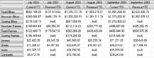
Note that even though I've removed the FORMAT() statement, we've retained the formatting—an artifact of summing formatted values. You could still put the statement back if you wanted to ensure how the numbers would be represented.