
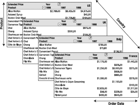
Cubes, dimensions, and measures are the fundamental parts of any OLAP solution. Let's consider the array of spreadsheets from Chapter 1, shown here again in Figure 2-1. At the most basic, the whole collection is a cube. In this chapter, you'll look at how this model relates to the concepts you need to grasp in order to understand OLAP and Analysis Services.
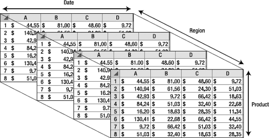
A cube is a collection of numeric data organized by arrays of discrete identifiers. Cubes were created to give a logical structure to the pivot table approach to analyzing large amounts of numerical data. Figure 2-1 shows how combining three variables creates a cube-like shape that we can work with. Although there are nuances to the design and optimization of cubes, all the magic is in that concept. A cube can (and generally will) have more than three variables defining it, but it will still always be referred to as a cube.
Note
Shifting from a programming mindset to an OLAP mindset can be difficult. In programming, a variable can have many values, but represents only one distinct value at a time. In OLAP, we are interested in analyzing a set of the possible values, so we work with an array of discrete values. In other words, the variable Region may have a single value of Missouri or Florida or Washington, but in an OLAP analysis we want to examine the set or array of possible region values: {Florida, Missouri, Washington}.
Essentially, a cube is defined by its measures and dimensions (more on them in a bit). Where the borders are drawn to define a cube is somewhat arbitrary, but generally a cube focuses on a functional area. Consider our order details spreadsheet from Figure 1-1 in Chapter 1—we have information on customers, their orders, products, and so forth.
Perhaps we also want to calculate cost of sales (that is, the amount we pay in expenses for every dollar of revenue we bring in). To get that information, we need to add in company financial data: building expenses, advertising, manufacturing or wholesale costs, shipping, and personnel salary and benefits information. Do we just pile all this stuff into our sales cube? This quickly becomes an issue of "throwing all your tools in one box." The problem is that later changes to the cube may affect a myriad of applications, as we have to consider interoperability of such changes, and so on. In addition, personnel financial information has significant privacy considerations; we can report on pay data in aggregate, but nothing that could identify any one person.
Instead, we consider adding the data in two cubes: one for corporate financial data (without personnel pay data), and one for HR data. Then we can link the data and parameters from the cubes as necessary so they stay synchronized.
From the aspect of defining a cube, either solution would work—one big huge cube or three smaller, subject-specific cubes. We prefer the latter situation, as this is more in-line with the data mart, or business area approach mentioned in Chapter 1. Your cubes will be easier to enhance and maintain using this approach. In theory, we could have a sales cube and an HR cube and split corporate financial data between them. We would likely regret this decision later, but we would still have two cubes.
Thinking back, what makes each of these so-called cubes really a cube? Each is a collection of numeric data (for example, sales totals, expense costs, personnel pay) grouped by arrays of discrete identifiers. For example, the following is a list of possible identifiers in different categories:
- Products:
mutton, crabmeat, chai, filo mix
- Countries:
France, Italy, United Kingdom, United States
- Dates:
1996, 1997, 1998
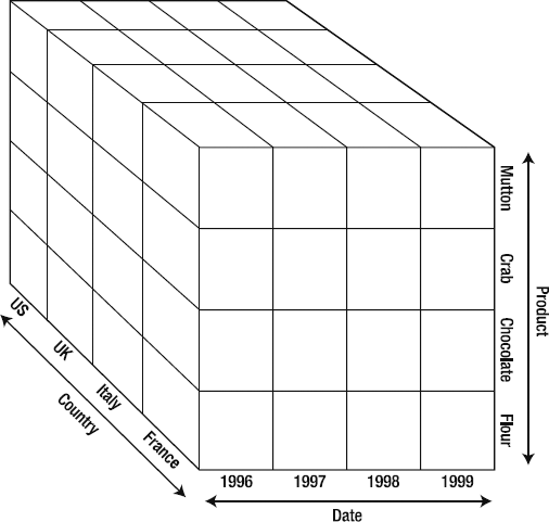
These categories are dimensions—the arrays of identifiers (members) that we use to analyze our data. By choosing different dimensions, we break up the data in different ways. Let's take another look at our "collection of spreadsheets" from Figure 2-1 with some more detail and a shift in perspective (Figure 2-2).
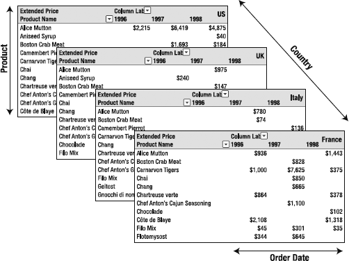
Again we can see that we have broken down our numbers by country, by year, and by product, and we can see the cube shape that gives cubes their name. We can see that the amount of Alice mutton sold in France in 1996 is $936. So we have a member from each of three dimensions to get a single value. That value is a measure.
Measures are the numeric data "inside" a cube. They define the data we get by selecting members from dimensions. Generally, measures are added together to produce summary results. In the cube in Figure 2-2, for example, the measure of Alice mutton sold in France in 1996 is obtained by adding together that line item from every order that month during that year. If we wanted to know all the sales in France in 1996, we'd add in the amounts for all the products and get a total that way (that is, the value of the Sales measure for the France member of the Country dimension and the 1996 member of the Order Date dimension).
If you've done a significant amount of programming or database administrator (DBA) design work, you will recognize that the year values in Figure 2-2 are best represented as text, or strings. If you entered 1996 as a number in Excel, Excel may format it as 1,996. Why do I bring this up? To clarify the next point I'm going to make:
Dimensions are strings; measures are numbers.
The most confusing part about cube design is the question "What's a measure, and what's a dimension?" I've found that this single reminder—that dimensions are strings, and measures are numbers—always keeps me straight. (At times measures are text, but they are an edge case I'll cover later.) You might be tempted to ask, "What if I want to break down my data by age? Age is a number." This is true, but consider how we've defined a cube, and measures, and dimensions. When using age as a dimension, you don't add the numbers; you use them as discrete labels. You probably wouldn't even use the individual numbers. You would create brackets such as the following:
1–18 Years
19–40 Years
41–65 Years
65+ Years
If you look at it that way, each member is, indeed, a string.
Another approach I often use (and almost always use when designing a staging database for a cube) is that dimensions are often directly linked to lookup tables. Again, thinking in terms of lookup tables, you can see that what makes a dimension becomes pretty clear.
Now that you have a basic understanding of cubes, measures, and dimensions, let's dig deeper into aspects of defining measures and dimensions in the OLAP world. In this section, you'll look at how dimensions relate to data, learning about schemas as the layer between a cube and a data source. Then you'll learn about dealing with hierarchical relationships (such as countries, states/regions, and cities) and time in OLAP. You'll also look at the question "If a member is a noun, where do we put the adjectives?" Finally, you'll dig more deeply into measures.
Just as pivot tables derive from relational data tables, the underlying structure of a cube is a collection of tables in a relational database. In the OLAP field, we label tables as either fact tables or dimension tables. A fact table contains data that yields a measure. A dimension table contains the lookup data for our dimensions. If a table contains both fact and dimension information (for example, an order details table will probably contain both the dollar amounts of the order and the items that were ordered), we still just call it a fact table.
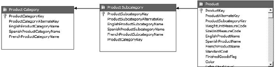
There are generally two types of schemas, or data structures, that cubes are built on: star and snowflake schemas. You'll see a lot of discussion devoted to these two structures, and might assume there is a huge amount of complexity to differentiating the two. Figure 2-3 shows a star schema with fact and dimension tables labeled. Figure 2-4 shows a snowflake schema.
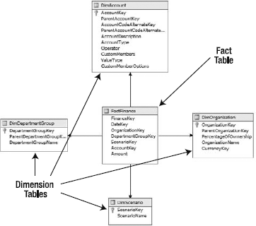
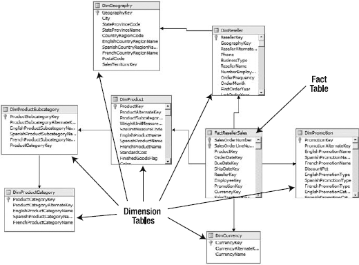
So what's the difference between a star schema and a snowflake schema? Yes, it's as easy as it appears. A star schema has one central fact table, with every dimension table linked directly to it. A snowflake schema is "everything else." In a typical snowflake schema, dimension tables are normalized, so hierarchies are defined via multiple related tables. For example, Figure 2-4 indicates a hierarchy for products, which is detailed in Figure 2-5. That's the entirety of the difference between star schemas and snowflake schemas—whether dimensions are represented by single tables or a collection of linked tables. (More-complex snowflake schemas can have multiple fact tables and interlinked dimensions. The AdventureWorks schema that we'll be using in Analysis Services is like this.)
Basically, snowflake schemas can be easier to model and require less storage space. However, they are more complex and require more processing power to generate a cube. Snowflake schemas can also make data transformation and loading into your staging tables more cumbersome. In addition, working with your slowly changing dimensions may also become more complex. (You'll learn more about slowly changing dimensions later in this chapter.)
Star schemas are generally easier for end users to work with and visualize, because they can easily see the dimensions involved. Finally, some products designed to work with OLAP technologies may restrict which type of schema they will work with. (Microsoft's PerformancePoint Business Modeler will work only with star schema models, for example.)
As I mentioned previously, the best way to think of a dimension is as a lookup table. A string is the member of the dimension. The dimension is represented by the unique array of values in that string field, and they are linked to the fact table with a primary key–foreign key relationship.
The concept of what makes a dimension, however, isn't as restrictive as a lookup table. Dimensions can derive from columns within the fact table, from related tables that contain data, from lookup tables, or even from tables that are related through a third table (reference relationship). Remember that the focus is on relating the array of dimension members to the measures that derive from the fact table, and don't get hung up on the implementation under the covers. Conceptually, dimensions are fairly straightforward, but several possible twists are covered in the next few sections.
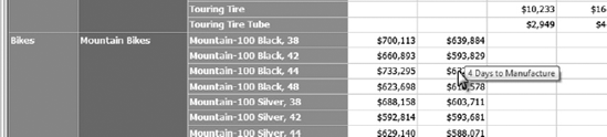
Attributes are metadata that belong to a dimension, and are used to add definition to the dimension members. In our ongoing example of orders management, a product member may have attributes giving details about the product (color, weight, description—even an image of the product). A customer dimension may have attributes giving address information, the length of time that person has been a customer, and other related information. Figure 2-6 shows a dimensional report (using SQL Server Reporting Services) that has a tool tip showing the number of days it takes to manufacture a product, using an attribute from the product dimension.
Attributes can also be used to calculate values. For example, consider a cube used to analyze consulting hours. Hours billed is the measure, and you may have dimensions for time, customer, consultant, and billing type. The consultant dimension could have an attribute of Hourly Rate that you can use to multiply by the hours to get the total amount billed, for analysis purposes.
Which brings us to another issue: hourly rates change over time. Other aspects of our business change over time (heck, what doesn't change over time?). To deal with that, we have slowly changing dimensions, often abbreviated as SCD.
Slowly changing dimensions deal with the reality that things change. Product definitions change; sales districts change; pricing changes; managers change; and customers change. Working with changing dimensions in a cube is fairly similar to working with changing lookup values in a relational database, with similar pros and cons.
Working well with SCDs requires methodologies for managing them—balancing manageability against the need to maintain (and report on) historical data. There are six methodologies for managing SCDs:
- Type 0
isn't really a management methodology, per se. It's simply a way to indicate that there's been no attempt to deal with the fact that the dimension changes. (Most notably, when a dimension that was expected to remain static changes, it effectively becomes a Type 0 SCD.)
- Type 1
simply replaces the old data with the new values. Thus any analysis of older data will show the new values. This is generally appropriate only when correcting dimension member data that is in error (misspelled, for example). This is obviously easy to maintain, but shows no historical data and may result in incorrect reports.
- Type 2
uses To and From dates in the member record, with the current date having a null End Date field. OLAP engines can implement logic to bind measure values to the appropriate dimension value transparently. Obviously, the need to maintain beginning and end dates, with only one null end date, makes data transformations for this method more complex. Type 2 is the most common approach to dealing with slowly changing dimensions.
- Type 3
is completely denormalized—it maintains the history of values and effective date in the record for the dimension, each in its own column. Given the need to track multiple columns of data, it's best to reserve this method for a small number of changes (for example, original value and current value without tracking interim changes). Because this is a simpler approach, it makes data transformations easier, but it's pretty restrictive.
- Type 4
uses two tables for dimensions: the standard dimension table, and a separate table for historical values. When a dimension value is updated, the old value is copied to the history table with its begin and end dates. This structure makes for the fastest processing of OLAP cubes and queries, while allowing for unlimited history. But again, transforming data and maintenance are problematic.
- Type 6
is a combination of Types 1, 2, and 3 (1 + 2 + 3 = 6; someone had a sense of humor). The dimension table has start and end dates (Type 2), adds attributes so that any historical data can be analyzed using the current "today" data (Type 1), or any mix of the two (Type 3).
Again, slowly changing dimensions are not that complex a topic to understand. The trick is in the analysis and implementation. You'll examine proper implementation of SCDs in Analysis Services later in the book. For our next challenge, what do we do when there is a hierarchy (parent-child relationship) in a dimension?
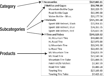
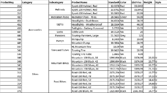
In the section on schemas, you looked at stars and snowflakes, with the main difference being that snowflakes use multiple tables to define dimensions. As I mentioned, you use snowflake schemas to implement a hierarchy—for example, Categories have Subcategories, and Subcategories have Products, as shown in Figure 2-7.
In a snowflake schema, the dimension could be built exactly like this: three tables, one for each level. In a star schema, we would denormalize the tables into a single dimension table similar to that shown in Figure 2-8.
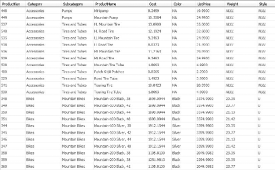
With the single-table approach, the Subcategory and Category fields will become attributes in the Product dimension. From there, you will create a hierarchy by using the attributes—using the Category attribute as the parent, the Subcategory as its child, and finally the Product as the child of the Subcategory attribute. Other attributes in the dimension will remain associated with the product. The end result is shown in Figure 2-9.
OLAP engines separate the creation of hierarchies from the underlying dimension data. Hierarchies are created by arranging relationships between attributes in the dimension. For example, in the table in Figure 2-8, you could create a hierarchy by linking Category to Subcategory, then to ProductName. Then either the designer or the engine would create a hierarchy by inferring the one-to-many relationships between categories, subcategories, and products. This approach means that fields can be reused in various hierarchies, so long as there is always a one-to-many relationship from top to bottom.
Tip
When you use hierarchies with cubes, some tools require what is referred to as the leaf level of the hierarchy. This simply means that if you use a hierarchy, you must select it down to the lowest level. For instance, in our category-subcategory-product hierarchy we've been working with, the product level is the leaf level.
Another consideration regarding hierarchies is whether a hierarchy will be balanced or unbalanced. In a balanced hierarchy, every branch descends to the same level. Our category-subcategory-product hierarchy is a balanced hierarchy, because every branch ends with one or more products. We don't have subcategories without products, or categories without subcategories.
An unbalanced hierarchy has branches that end at different levels. Organizational hierarchies are often unbalanced. Although some branches may descend from CEO to VP to Director to Manager to Employee, there will be directors with nobody working for them. That branch will just be CEO to VP to Director.
One other hierarchy that comes to mind is a calendar, in which you'll have years, quarters, months, weeks, and days. However, the calendar is a special case, as it impacts many areas of a cube. Let's take a look at the time dimension. (Cue theremin. Yes, go look it up.)
A lot of analysis of OLAP data is financial in nature and performed by the green-eyeshade people. A lot of financial analysis turns out to be time based. They want calculations such as rolling averages, year over year change, quarter to date attainment, and so on. Rolling averages are actually fairly straightforward, as you just need to take the data from the last x number of days. But what about quarter to date? On February 15, we want to add the data from January 1 through today. On March 29, it's January 1 through March 29. But on April 1, we just use the data from April.
I have known groups that update their reports every quarter to deal with this situation. A better but still painful solution is to write a query that determines the current quarter, determines the first date of the current quarter, and then uses that to restrict the data in a subquery. However, you have to consider that this calculation has to be run for every value or set of values in the report.
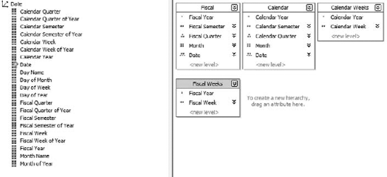
OLAP engines provide a time-based analysis capability that makes these types of reports easy. First, as I mentioned in the previous section, is the hierarchical aspect of a time dimension: years, quarters, months, days. In addition, the ability to have multiple hierarchies on a single set of dimension members comes into use here; you can have a hierarchy of year-month-day coexist with year-week-day. More important, you can have multiple calendars: a standard calendar, in which the year runs from January 1 to December 31, and a fiscal calendar, which runs from the start of the fiscal year to the end (each with halves, quarters, weeks, and so forth). You might also have a manufacturing calendar, or an offset calendar for another reason. Figure 2-10 shows the attributes of a date dimension used in various hierarchies.
After we have a time dimension set up, we can leverage some powerful commands in the OLAP query language, MDX (more on MDX later). For now, it's sufficient to understand that MDX, when coupled with a time dimension, enables an analyst to create queries for aggregations of data such as year to date, a running average, or parallel periods (aggregate totaled over the same period in a previous year, for example). After the query is established, the OLAP engine automatically calculates the time periods as the calendar moves on.
You'll look at time analysis of data in Chapter 10. In the meantime, you need to understand what data, and what aggregations, are at the center of our attention. Let's take a look at the center of the cube: measures.
At the root of everything we're trying to do are measures, or the numbers we're trying to analyze. As I stated earlier, generally measures are numbers—dollars, days, counts, and so forth. We are looking at values that we want to combine in different ways (most commonly by adding):
How many bananas do we sell on weekdays vs. weekends?
What color car sells best in summer months?
What is the trend in sales (dollars) through the year, broken down by sales district?
How many tons of grain do our livestock eat per month in the winter?
In each of these cases, we'll have individual records of sales or consumption, which we can combine. We'll then create dimensions and select members of those dimensions to answer the question.
Tip
OLAP engines will automatically provide a count measure for you based on the number of members of a dimension. It is effectively summing a 1 for every record in the collection of records returned. Extrapolating from this, you can see it's possible to create a subset count. For example, if you had a cube representing an automobile inventory, you could create a total of low-emission vehicles (LEVs) by having a column for LEVs and placing a 1 in the column for every LEV and a 0 for every other vehicle. By totaling the column in a query, you would have a count of the LEV vehicles.
Now that I've covered the fundamentals of a cube, let's visualize these aggregations. Figure 2-11 is our "collection of spreadsheets" cube. Note the dimensions: dates along the columns, products down the rows, and each page is a separate country.
Now let's look at the more abstract representation in Figure 2-12. You should be able to see the analogue pretty clearly.

Imagine that each small cube has a single numeric value inside it. When we want to do analysis, we use the dimensions, which each have a single member in each cube unit, as shown in Figure 2-13.
So, filling in the other dimensions, we have something similar to Figure 2-14.
Given this structure, let's say we want to know the total sales of mutton in Italy from 1996–1998. Figure 2-15 should give you an idea of where we're going with this.
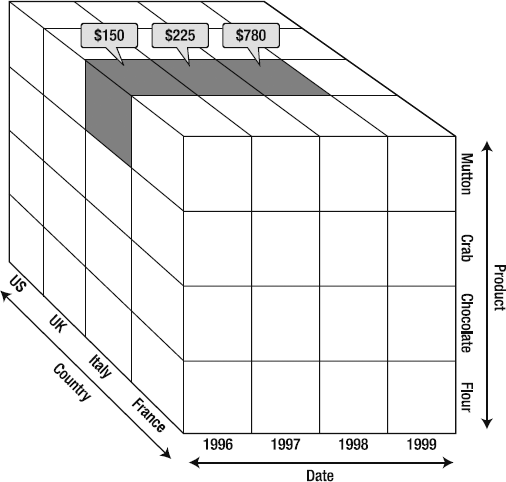
As you can see, by selecting the members of various dimensions, we select a subset of the values in the whole cube. The OLAP engine responds by returning a set of values corresponding to the members we've selected, that is, {$150, $225, $780}. Each of those values will be an aggregation. For example, mutton sold in Italy in 1996 was returned as $150; that may consist of $75 bought by one customer, $35 by another, and $40 by a third. Now imagine that we want to see the amount of mutton sold in Italy and France in 1996 and 1997 (Figure 2-16). The OLAP engine will return an array we can use for reporting, calculations, analysis, and so forth. (You can already see that France outsold Italy in each year. Perhaps additional investigation is needed?)
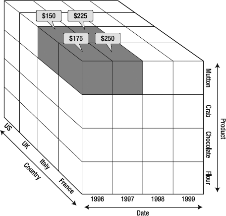
To further analyze the results, we may drill into the date hierarchy to see how the numbers compare by quarter or month. We could also compare these sales results to the sales of other products or number of customers. Maybe we'd like to look at repeat customers in each area (is France outperforming Italy on attracting new customers, bringing back existing customers, or both?). All these questions can be answered by leveraging various aspects of this cube.
Incidentally, selection of various members is accomplished with a query language referred to as Multidimensional Expressions, or more commonly MDX. You'll be looking at MDX in depth in Chapter 9.
A question that may have come to mind by now: "Are measure values always added?" Although measures are generally added together as they are aggregated, that is not always the case. If you had a cube full of temperature data, you wouldn't add the temperatures as you grouped readings. You would want the minimum, maximum, average, or some other manner of aggregating the data. In a similar vein, data consisting of maximum values may not be appropriate to average together, because the averages would not be representative of the underlying data.
OLAP offers several ways of aggregating the numerical measures in our cube. But first we want to designate how to aggregate the data—either additive, nonadditive, or semiadditive measures.
An additive measure can be aggregated along any dimension associated with the measure. When working with our sales measure, the sales figures are added together whether we use the date dimension, region, or product. Additive measures can be added or counted (and the counts can be added).
A semiadditive measure can be aggregated along some dimensions but not others. The simplest example is an inventory, which can be added across warehouses, districts, and even products. However, you can't add inventory across time; if I have 1,100 widgets in stock in September, and then (after selling 200 widgets) I have 900 widgets in October, that doesn't mean I have 2,000 widgets (1,100 + 900).
Finally, a nonadditive measure cannot be aggregated along any dimension. It must be calculated independently for every set of data. A distinct count is an example of a nonadditive measure.
Note
SQL Server Analysis Services has a semiadditive measure calculation named AverageOfChildren. You might be confused about why this is considered semiadditive. It turns out that the way this aggregation operates is that it sums along every dimension except a time dimension; along the time dimension, it averages (covering the inventory example given earlier).
Most of the time OLAP cubes are implemented, they are put in place as an analytic tool, so cubes are read-only. On some occasions, users may want to write data back to the cube. We don't want users changing inventory or sales numbers from an analysis tool, so why would they want to change the numbers?
A powerful analysis technique to offer your users is what-if or scenario analysis. Using this process, analysts can change numbers in the cube to evaluate the longer-term effects of those changes. For example, they might want to see what happens to year-end budget numbers if every department cuts its budget by 10 percent. What happens to salaries? Capital expenses? Recurring costs? Although these effects can be run with multiple spreadsheets, you could also create an additional dimension named scenario, which analysts can use to edit data and view the outcomes. The method of committing those edits is called writeback.
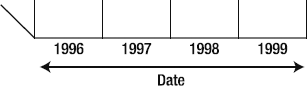
The biggest concern when implementing writeback on a cube is dealing with spreading. Consider our time dimension (Figure 2-17). An analyst who is working on a report that shows calendar quarters might want to change one value. When that value is changed, what do we do about the months? The days?
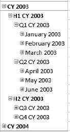
We have two choices. In our design, we can create a dimension that drills down to only the quarter level. Then the calendar quarters are the leaf level of the dimension, the bottom-most level, and the value for the quarter is just written into the cell for that quarter. Alternatively, some OLAP engines will allow the DBA to configure a dimension for spreading; when the engine writes back to the cube, it distributes the edited value to the child elements. The easiest (and usually default) option is to divide the new value by the number of children and divide it equally. An alternative that may be available if the analyst is editing a value is to distribute the new value proportionally to the old value.
Writeback in general, and spreading in particular, are both very processor- and memory-intensive processes, so be judicious about when you implement them. You'll look at writeback in Analysis Services in Chapter 11.
Often you'll need to calculate a value, either from values in the measure (for example, extended price calculated by multiplying the unit cost by the number of items), or from underlying data, such as an average.
Calculating averages is tricky; you can't simply average the averages together. Consider the data in Table 2-1, showing three classes and their average grades.
Table 2.1. Averaging Averages
Classroom | Number of Students | Average Score |
|---|---|---|
Classroom A | 20 | 100% |
Classroom B | 40 | 80% |
Classroom C | 80 | 75% |
You can't simply add 100, 80, and 75 then divide by 3 to get an average of 85. You need to go back to the original scores, sum them all together, and divide by the 140 students, giving an answer of 80 percent. This is another area where OLAP really pays off, because the OLAP engine is designed to run these calculations as necessary, meaning that all the user has to worry about is selecting the analysis they want to do instead of how it's calculated.
Generally, an OLAP solution is the first-layer approach to analysis—it's where you start. After you find something of interest, you generally want additional information. One method of getting amplifying data for something you find in an analysis is to drill through to the underlying data. Some analysis tools provide a way of doing this directly, at least to the fact table; others don't.
A more general way of gaining contextual insight into the data that you are looking at is to create a structure called an action. This enables an end user to easily view amplifying data for a given dimension member or measure. You can provide reports, drill-through data sets, web pages (Figure 2-18), or even executable actions.
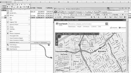
Actions are attached to objects in the cube—a specific dimension, hierarchy or hierarchy level, measure, or a member of any of those. If the object will have several potential targets (as a dimension has multiple members), you will have to set up a way to link the member to the target (parsing a URL, creating a SQL script, passing a parameter to a report). For example, Listing 2-1 shows code used to assemble a URL from the members selected in an action that opens a web-based map.
Example 2.1. Creating a URL from Dimension Members
// URL for linking to MSN Maps
"http://maps.msn.com/home.aspx?plce1=" +
// Retreive the name of the current city
[Geography].[City].CurrentMember.Name + "," +
// Append state-province name
[Geography].[State-Province].CurrentMember.Name + "," +
// Append country name
[Geography].[Country].CurrentMember.Name +
// Append region parameter
"®n1=" +
// Determine correct region parameter value
Case
When [Geography].[Country].CurrentMember Is
[Geography].[Country].&[Australia]
Then "3"
When [Geography].[Country].CurrentMember Is
[Geography].[Country].&[Canada]
Or
[Geography].[Country].CurrentMember Is
[Geography].[Country].&[United States]
Then "0"
Else "1"
EndThis code will take the members of the hierarchy from the dimension member you select to assemble the URL (the syntax is MDX, which you'll take a quick look at in a few pages and dig into in depth in Chapter 9). This URL is passed to the client that requested it, and the client will launch the URL by using whatever mechanism is in place.
Other actions operate the same way: they assemble some kind of script or query based on the members selected and then send it to the client. Actions that provide a drill-through will create a data set of some form and pass that to the client.
All these connections are generally via XMLA.
XML for Analysis (XMLA) was introduced by Microsoft in 2000 as a standard transport for querying OLAP engines. In 2001, Microsoft and Hyperion joined together to form the XMLA Council to maintain the standard. Today more than 25 companies follow the XMLA standard.
XMLA is a SOAP-based API (because it doesn't necessarily travel over HTTP, it's not a web service). Fundamentally, XMLA consists of just two methods: discover and execute. All results are returned in XML. Queries are sent via the execute method; the query language is not defined by the XMLA standard.
That's really all you need to know about XMLA. Just be aware of the transport mechanism and that it's nearly a universal standard. It's not necessary to dig deeper unless you discover a need to.
Note
For more information about XMLA, see http://msdn.microsoft.com/en-us/library/ms977626.aspx.
XMLA is the transport, so how do we express queries from OLAP engines? There were a number of query syntaxes before Microsoft introduced MDX with OLAP Services in 1997. MDX is designed to work in terms of measures, dimensions, and cubes, and returns structured data sets representing the dimensional nature of the cube.
In working with OLAP solutions, you'll work with both MDX queries and MDX statements. An MDX query is a full query, designed to return a set of dimensional data. MDX statements are parts of an MDX query, used for defining a set of dimensional data (for use in client tools, defining aspects of cube design, and so forth).
A basic MDX query looks like this:
SELECT [measures] ON COLUMNS,
[dimension members] ON ROWS
FROM [cube]
WHERE [condition]
Listing 2-2 shows a more advanced query, and Figure 2-19 shows the results from a grid in Excel.
Example 2.2. A More Advanced MDX Query
SELECT {DrilldownLevel({[Date].[Calendar Year].[All Periods]})} ON COLUMNS,
       {DrilldownLevel({[Geography].[Geography].[All Geographies]})} ON ROWS
FROM
(
   SELECT
      {[Geography].[Geography].[Country].&[United States],
      [Geography].[Geography].[Country].&[Germany],
      [Geography].[Geography].[Country].&[France]} ON COLUMNS
   FROM [Adventure Works]
)
WHERE ([Product].[Product Categories].[Category].&[1],[Measures].[Reseller Sales Amount])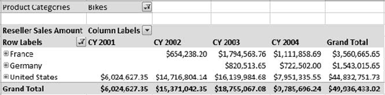
When working with dimensional data, you can write MDX by hand or use a designer. There are several client tools that enable you to create MDX data sets by using drag-and-drop, and then view the resulting MDX. Just as with SQL queries, you will often find yourself using a client tool to get a query close to what you're looking for, then tweak it manually from the MDX.
Chapter 9 covers MDX in depth.
Data warehouse is a term that is loosely used to describe a unified repository of data for an organization. Different people may use it to refer to a relational database or an OLAP dimensional data store (or both). Conceptually, the idea is to have one large data "thing" that serves as a repository for all the organization's data for reporting and analytic needs.
The data warehouse may be a large relational data store that unifies data from various other systems throughout the business, making it possible to run enterprise financial reports, perform analysis on numbers across the company (perhaps payroll or absentee reports), and ensure that standardized business rules are being applied uniformly. For example, when calculating absenteeism or consultant utilization reports, are holidays counted as billable time? Do they count against the base number of hours? There is no correct answer, but it is important that everyone use the same answer when doing the calculations.
Many companies perform dimensional analysis against these large relational stores, just as you can create a pivot table against a table of data in Excel. However, this neglects a significant amount of research and investment that has been made into OLAP engines. It is not redundant to put a dimensional solution on top of the relational store. Significant reporting can still be performed on the relational store, leaving the cube for dimensional analysis. In addition, the data warehouse becomes a staging database (more on those in a bit) for the cube. There are two possible approaches to building a data warehouse: bottom-up or top-down.
Bottom-up design relies on departmental adoption of numerous small data marts to accomplish analysis of their data. The benefit to this design approach is that business value is recognized more quickly, because the data marts can be put into use as they come online. In addition, as more data marts are created, business groups can blend in lessons learned from previous cubes. The downside to this approach is the potential need for redesign in existing cubes as groups try to unite them later. The software design analogy to bottom-up design is the agile methodology.
Top-down design attacks the large enterprise repository up front. A working group will put together the necessary unifying design decisions to build the data warehouse in one fell swoop. On the plus side, there is minimal duplication of effort as one large repository is built. Unfortunately, because of the magnitude of the effort, there is significant risk of analysis paralysis and failure. Top-down design is similar to software projects with big up-front or waterfall approaches.
Data warehouses will always have to maintain a significant amount of data. So storage configuration becomes a high-level concern.
Occasionally, you'll have to deal with configuring storage for an OLAP solution. One issue that arises is the amount of space that calculating every possibility can take. Consider a sales cube: 365 days; 1,500 products; 100 sales people; 50 sales districts. For that one year, the engine would have to calculate 365 × 1,500 × 100 × 50 = 2,737,500,000 values. Each year. And we haven't figured in the hierarchies (product categories, months and quarters, and so forth).
Another issue here is that not every intersection is going to have a value; not every product is bought in every district every day. The result is that OLAP is generally considered a sparse storage problem (for every cell that could be calculated, most will be empty). This has implications both in designing storage for the cube as well as optimizing design and queries for response time.
When designing an OLAP solution, you will generally be drawing data from multiple data sources. Although some engines have the capability to read directly from those data sources, you will often have issues unifying the data in those underlying systems. For example, one system may index product data by catalog number, another may do so by unique ID, and a third may use the nomenclature as a key. And of course every system will have different nomenclature for red ten-speed bicycle.
If you have to clean data, either to get everyone on the same page or perhaps to deal with human error in manually entered records (where is Missisippi?), you will generally start by aggregating the records in a staging database. This is simply a relational store designed as the location where you unify data from other systems before building a cube on top. The staging database generally will have a design that is more cube-friendly than your average relational system—tables arranged in a more fact/dimension manner instead of the normalized transactional mode of capturing individual records, for example.
Note
Moving data from one transactional system into another is best accomplished with an extract-transform-load, or ETL, engine. SQL Server Integration Services is a great ETL engine that is part of SQL Server licensing.
The next few sections cover storage of relational data; they are referring to caching data from the data source, not this staging database. It's possible to worry entirely too much about whether to use MOLAP, ROLAP, or HOLAP—don't. For 99 percent of your analysis solutions, your analysts will be using data from last month, last quarter, or last year. They won't be deeply concerned about keeping up with the data as it changes, because it's all committed and "put to bed." As a result, MOLAP will be just fine in all these cases.
ROLAP really becomes an issue only when you need continually updated data (for example, running analysis on assembly line equipment for the current month). Although it's important when it's needed, it's generally not an issue. Let's take a look at what each of these mean.
Multidimensional OLAP (MOLAP) is probably what you've been thinking of to this point—the underlying data is cached to the OLAP server, and the aggregations are precalculated and stored in the OLAP server as well. This approach optimizes response time for queries, but because of the precalculated aggregations, it does require a lot of storage space.
Relational OLAP (ROLAP) keeps the underlying data in the relational data system. In addition, the aggregations are calculated and stored in the relational data system. The benefit of ROLAP is that because it is linked directly to the underlying source data, there is no latency between changes in the source data and the analytic results. Some OLAP systems may take advantage of server caching to speed up response times, but in general the disadvantage of ROLAP aggregations is that because you're not leveraging the OLAP engine for precalculation and aggregation of results, analysis is much slower.
Hybrid OLAP (HOLAP) mixes MOLAP and ROLAP. Aggregations are stored in the OLAP storage, but the source data is kept in the relational data store. Queries that depend on the preaggregated data will be as responsive as MOLAP cubes, while queries that require reading the source data (aggregations that haven't been precalculated, or drilled down to the source data) will be slower, akin to the response times of ROLAP.
We'll review Analysis Services storage design in Chapter 12.