
Data-mining technologies provide business users with the means to analyze and sift through gargantuan amounts of information stored in corporate data warehouses. Data-mining tools implement a variety of algorithms that, when applied to the enterprise data warehouse (EDW), greatly aid the decision-making process. In today's hypercompetitive climate, adding mining to your analytics bag of tricks can help you find that "needle in the haystack" prediction that puts your ability to act ahead of your competitors'.
In this chapter, you will create and apply mining models to the AdventureWorks data warehouse. These models will be used to predict buyers of AdventureWorks products. While predicting buyers, you will discover not only potential customers, but the products they are most interested in. Finally, you will analyze the possible sales growth to AdventureWorks from these customers. You'll see how to create models that help you find a niche or an entirely new way to grow your business.
Data mining provides a powerful decision support mechanism. Data mining is used in virtually every industry by marketing departments, customer relationship management groups, network (e-mail) security, finance/credit departments, human resources (employee performance), and others.
The following examples offer a few ways that I have seen data mining used:
- Loss mitigation:
A finance company mined data related to customer payment, auction sale recovery, auction sale expenses, customer income, and demographics to predict future troubled accounts. This data was used to predict repossession and auction probabilities. Based on the discoveries made, collection activities were focused on the customers most likely to perform in the future. For loans that were predicted not to perform, new loan modification products and processes were created and actively presented to the at-risk borrowers.
- Cost reduction:
A remanufacturing company mined manufacturer repair data, bill of materials (BOM) usage, parts cost trending, and parts availability trending to predict future costs of goods for each product refurbished. One outcome of this effort resulted in the creation of new business processes at the receiving dock, which included holding back product from technician workstations that did not have parts in stock. This change alone improved service-level agreement (SLA) performance to manufacturers by reducing turn-around time for products with stocked parts. In addition, these process updates improved costs by allowing technicians to focus on their part of the remanufacturing process.
- Worldwide strategic marketing:
A telecom equipment manufacturer mined government data for cell phones owned, computers owned, and gross income at the regional, national, and per-capita level. Competitive data was also gathered/purchased that provided service provider penetration and relationships; larger providers own chunks of smaller ones. These efforts resulted in an extremely focused marketing plan, targeting second-tier service providers in emerging economies, and resulted in several successes in the Chinese and Brazilian marketplaces.
- Education:
An independent school district mined statewide standardized testing scores and other demographic data to predict students at risk of underperforming or failing these tests at the grade and subject levels. These efforts resulted in a new initiative by the district to group at-risk students together, not only in smaller classes, but in smaller classes focused on the particular subjects these students were struggling in. Along with this, teacher assignments were reevaluated to enable teachers who performed better with at-risk students to head these classes. Not only did test scores show improvement, but discipline-related issues decreased as well.
The mining algorithms implemented in SSAS are your core toolset for creating predictive models. In this section, I describe a few of the more essential data-mining algorithms and their general purpose. For each algorithm, I introduce the algorithm type and define three data requirements: input data, the key column, and the prediction column.
The Microsoft Naïve Bayes algorithm creates classification predictions. The Naïve Bayes algorithm is simply a true-or-false mechanism, and does not account for any types of dependencies that may exist in the data you are analyzing. In order to create a Naïve Bayes model, you need to prepare your data and create a training data set. This need for a training data set marks Naïve Bayes as one of the supervised mining algorithms.
A Microsoft Naïve Bayes model requires the following training data:
- Input:
Input data columns must be discretized, because Naïve Bayes is not designed to be used with continuous data, and your inputs should be fairly independent of each other. One method of discretization is known as banding, or binning, data. Two common examples of banding data include age and income. Age is often discretized as Child, Teenager, Adult, and Senior Citizen. It may also be banded as < 11, 12–17, 18–54, and 55+. Income is often banded in brackets, such as < 20,000, 20,000–50,000, and 50,000+.
- Key column:
A unique identifier is required for each record in the training set. Two examples of unique identifiers are a surrogate key and a globally unique identifier (GUID). A surrogate key in the EDW is usually a SQL Server Identity column, which is basically a numeric counter, guaranteed to be unique by the database engine.
- Prediction column:
This is the the prediction attribute. Will the customer buy more of our products? Is the applicant a good credit risk?
Microsoft Clustering is a segmentation algorithm. It creates segments, or buckets, of groups that have similar characteristics, based on the attributes that you supply to the algorithm. Microsoft Clustering uses equal weighting across attributes when creating segments. Many times, these segments may not be readily apparent but are important nonetheless.
A Microsoft Clustering model requires the following:
- Input:
Input data columns for this algorithm can be continuous in nature. Continuous input is represented by the
Date,Double, andLongdata types in SQL Server. These data types can be divided into fractional values.- Key column:
A unique identifier is required for each record in the training set. Two examples of unique identifiers are a surrogate key and a GUID. A surrogate key in the EDW is usually a SQL Server Identity column, which is basically a numeric counter, guaranteed to be unique by the database engine.
- Prediction column:
This is the the prediction attribute. Use of a prediction column is optional with this algorithm. Segments will be created automatically by the algorithm when a prediction column is not supplied. I suggest trying this with every Clustering model you make. It may teach you something you did not know about your data!
The Microsoft Decision Trees algorithm creates predictions for classification and association. A decision tree resembles the structure of a B-tree. As part of the data-mining business process, decision trees are often run against individual segments from a Clustering model.
A Microsoft Decision Tree model requires the following:
- Input:
Input data can be either discrete or continuous.
- Key column:
Like Naïve Bayes and Clustering, a unique identifier is required for each record in the training set.
- Prediction column:
This is the prediction attribute. It can be either discrete or continuous for this algorithm. If you use a discrete attribute, the tree can be well represented by a histogram.
Note
Prediction columns have two possible settings: Predict and PredictOnly. PredictOnly columns, as the name suggests, attempt to create predictions on the column chosen. A Predict column, on the other hand, uses the chosen data point to train your model as well.
The AdventureWorks marketing group has come to you for their next campaign. The Bike Buyers campaign has completed successfully, and your management would like to build on this success.
For the remainder of this chapter, you will create data-mining models using the AdventureWorks data warehouse. You will create three models to support the launch of the Accessory Buyers campaign, which is being created to supplement the recently concluded Bike Buyers campaign.
You will use a different method to create each of the needed models. First, you will use the Data Mining Wizard to create a mining model. Second, you will use Data Mining Extensions (DMX) to generate a mining model, and last, you will create a mining model by using an existing AdventureWorks cube.
Your first step is to discuss this campaign in more detail with your marketing group. Based on these discussions and further review of the Bike Buyers campaign, you've decided that bike buyers always buy helmets with a new bicycle. The marketing group states that the reasons for this are twofold: first, bike buyers want a helmet to match the new bicycle, and second, local laws in many areas prohibit riding a bicycle without a helmet. In addition, marketing asks that you include the Clothing product category in this campaign.
With the requirements in mind, you decide on two views in the AdventureWorks DW2008 database: vDMPrepAccessories and vAccessoryBuyers. These two new views are based on the original vDMPrep and vTargetMail views that already exist.
The first view, vDMPrepAccessories, is listed here:
--      Purpose:        Create vDMPrepAccessories
Use AdventureWorksDW2008
GO

If      Exists
(
   Select * From sys.views Where object_id = OBJECT_ID(N'dbo.vDMPrepAccessories')
)
   Drop View dbo.vDMPrepAccessories
GO

Create View dbo.vDMPrepAccessories
As

Select
   PC.EnglishProductCategoryName,
   PSC.EnglishProductSubcategoryName,
   Coalesce(P.ModelName, P.EnglishProductName) As Model,
   C.CustomerKey,
   S.SalesTerritoryGroup As Region,

   Case
      When Month(GetDate()) < Month(C.BirthDate)
         Then DateDiff(yy, C.BirthDate,GetDate()) - 1
      When Month(GetDate()) = Month(C.BirthDate) And Day(GetDate()) < Day(C.BirthDate)
         Then DateDiff(yy, C.BirthDate,GetDate()) - 1
      Else DateDiff(yy, C.BirthDate,GetDate())
   End As Age,

   Case
      When C.YearlyIncome < 40000
         Then 'Low'
      When C.YearlyIncome > 60000
         Then 'High'
Else 'Moderate'
End As IncomeGroup,
D.CalendarYear,
D.FiscalYear,
D.MonthNumberOfYear As Month,
F.SalesOrderNumber As OrderNumber,
F.SalesOrderLineNumber As LineNumber,
F.OrderQuantity As Quantity,
F.ExtendedAmount As Amount
From
dbo.FactInternetSales F Inner Join
dbo.DimDate D On
F.OrderDateKey = D.DateKey Inner Join
dbo.DimProduct P On
F.ProductKey = P.ProductKey Inner Join
dbo.DimProductSubcategory PSC On
P.ProductSubcategoryKey = PSC.ProductSubcategoryKey Inner Join
dbo.DimProductCategory PC On
PSC.ProductCategoryKey = PC.ProductCategoryKey Inner Join
dbo.DimCustomer C On
F.CustomerKey = C.CustomerKey Inner Join
dbo.DimGeography G On
C.GeographyKey = G.GeographyKey Inner Join
dbo.DimSalesTerritory S On
G.SalesTerritoryKey = S.SalesTerritoryKey
Where
PC.EnglishProductCategoryName Not In ('Bikes','Components') And
PSC.EnglishProductSubcategoryName Not In ('Helmets')
GoThis code creates the vDMPrepAccessories view that you will be using throughout the rest of this chapter. This view joins several tables in the AdventureWorks DW2008 database, and creates three bands for YearlyIncome. Finally, the view will return only accessories that are not Helmets.
The second view, vAccessoryBuyers, is listed here:
-- Purpose: Create vAccessoryBuyers Use AdventureWorksDW2008 GO If Exists( Select * From sys.views Where object_id= OBJECT_ID(N'dbo.vAccessoryBuyers')) Drop View dbo.vAccessoryBuyers GO Create View dbo.vAccessoryBuyers As Select C.CustomerKey, C.GeographyKey, C.CustomerAlternateKey,
C.Title,
   C.FirstName,
   C.MiddleName,
   C.LastName,
   C.NameStyle,
   C.BirthDate,
   C.MaritalStatus,
   C.Suffix,
   C.Gender,
   C.EmailAddress,
   C.YearlyIncome,
   C.TotalChildren,
   C.NumberChildrenAtHome,
   C.EnglishEducation,
   C.SpanishEducation,
   C.FrenchEducation,
   C.EnglishOccupation,
   C.SpanishOccupation,
   C.FrenchOccupation,
   C.HouseOwnerFlag,
   C.NumberCarsOwned,
   C.AddressLine1,
   C.AddressLine2,
   C.Phone,
   C.DateFirstPurchase,
   C.CommuteDistance,
   D.Region,
   D.Age,

   Case D.Clothing
      When  0  Then  0
      Else  1
   End As ClothingBuyer,

   Case D.Accessories
      When  0  Then  0
      Else  1
   End As AccessoryBuyer
From
   dbo.DimCustomer As C Inner Join
   (
      Select
         CustomerKey,
         Region,
         Age,

         Sum(Case EnglishProductCategoryName
               When  'Clothing'     Then  1
               Else  0
            End)  As Clothing,

         Sum(Case EnglishProductCategoryName
When 'Accessories' Then 1
Else 0
End) As Accessories
From
dbo.vDMPrepAccessories
Group By
CustomerKey,
Region,
Age
) As D On
C.CustomerKey = D.CustomerKey
GOThis code creates the vAccessoryBuyers view that we will be using throughout the rest of this chapter. This view joins DimCustomer to a derived table, D, which is based on the vDMPrepAccessories view you created earlier. You now have your ClothingBuyer and AccessoryBuyer data points.
In addition to the views defined in the preceding section, you will need a new data source view (DSV) that references the vAccessoryBuyers view and the ProspectiveBuyer table. The ProspectiveBuyer table is populated with your campaign targets. In Exercise 11-1, you will create the AccessoryCampaign DSV. Because this DSV is virtually identical to the one you created in Chapter 5, I will list the instructions only, without the dialog box figures.
Now that you have your views implemented, your next exercise is to create a new data-mining model. Do that by following the steps in Exercise 11-2. You will use the Microsoft Decision Trees algorithm to mine the AdventureWorks data warehouse. Your goal is to find a target population of potential accessory buyers.
Use the Data Mining Wizard
Follow these steps to create a data-mining model:
Open the AdventureWorks solution that you've been using for these exercises.
Right-click the Mining Structures folder in the Solution Explorer pane, and click New Mining Structure. The Data Mining Wizard introduction dialog box appears; click Next.
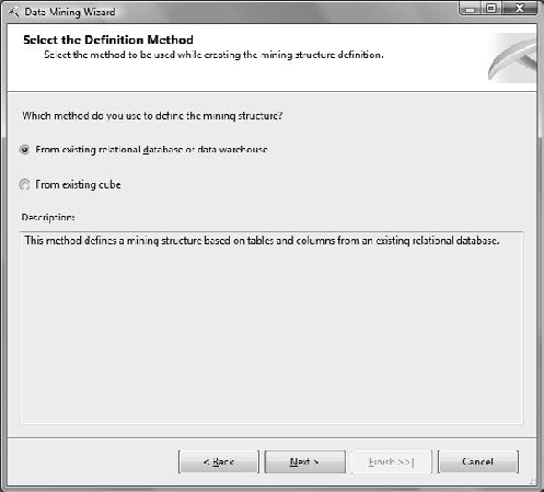
The Select the Definition Method dialog box appears, as shown in Figure 11-1; choose From Existing Relational Database or Data Warehouse, and click Next.
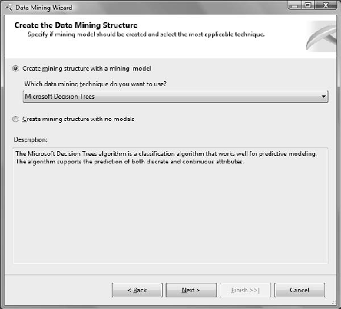
In the Create the Data Mining Structure dialog box, shown in Figure 11-2, leave Create Mining Structure with a Mining Model selected, and choose Microsoft Decision Trees from the Which Data Mining Technique Do You Want to Use drop-down. Click Next.
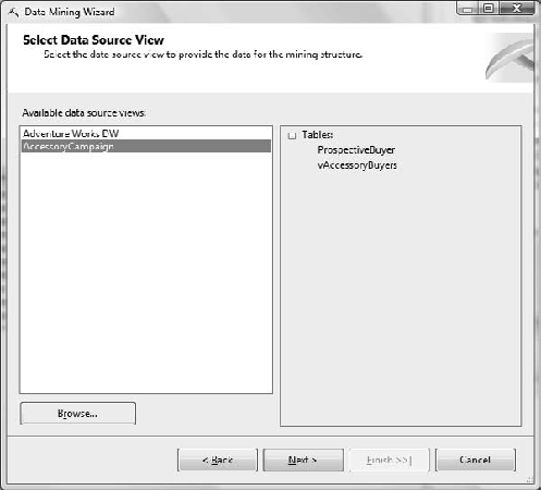
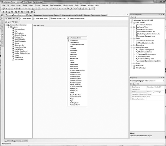
In the Select Data Source View dialog box, shown in Figure 11-3, choose AccessoryCampaign from your Available Data Source Views, and click Next.
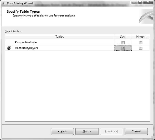
You will now see the Specify Table Types dialog box. As shown in Figure 11-4, select the Case check box for vAccessoryBuyers. Click Next.
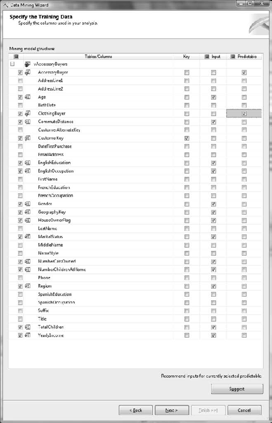
Now you get to think about the actual analysis you'll be doing. In the Key column, leave CustomerKey selected as your Key. For your Input columns, choose the following thirteen fields: Age, CommuteDistance, EnglishEducation, EnglishOccupation, Gender, GeographyKey, HouseOwnerFlag, MaritalStatus, NumberCarsOwned, NumberChildrenAtHome, Region, TotalChildren, and finally YearlyIncome. This model requires two Predictable columns; choose AccessoryBuyer and ClothingBuyer. Your selections should mimic Figure 11-5. When you are finished, click Next.
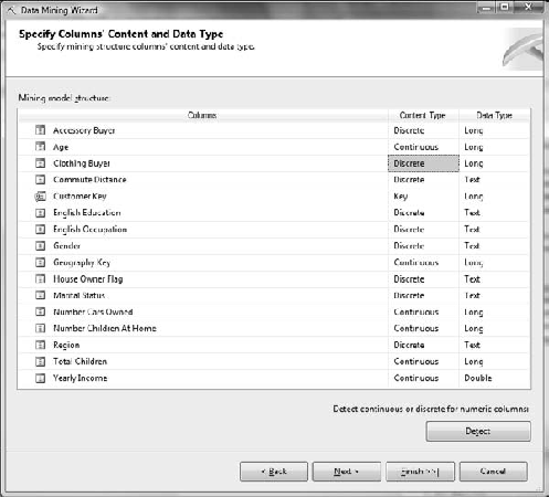
In the Specify Columns' Content and Data Type dialog box, shown in Figure 11-6, there are two changes that you need to make. Change Accessory Buyer and Clothing Buyer to Discrete in the Content Type column. Click Next.
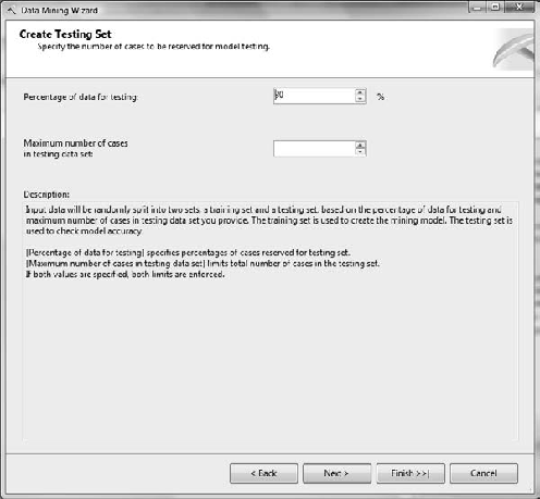
The Create Testing Set dialog box, shown in Figure 11-7, is where you will specify some inputs regarding how you would like your model to be trained. For this exercise, leave the Percentage of Data for Testing option set to 30 percent, and Maximum Number of Cases in Testing Data blank. Click Next.
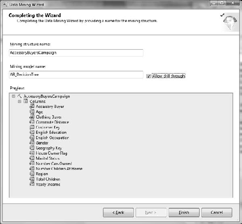
Now you can finalize your wizard entries by entering a name for your structure and model. Enter AccessoryBuyersCampaign as your Mining Structure Name and AB_DecisionTree for your Mining Model Name. Finally, as shown in Figure 11-8, be sure to select the Allow Drill Through check box. Click Finish.
After the wizard completes, the Data Mining Model Designer will fill your workspace. Next, you will explore the functionality of each of the five tabs within the designer.
The Data Mining Model Designer will be your main work area, now that you have finished defining your model with the Data Mining Wizard. The Data Mining Model Designer consists of the following tabs:
- Mining Structure:
This is where you modify and process your mining structure.
- Mining Models:
Here you create or modify models from your mining structure.
- Mining Model Viewer:
This view enables you to explore the models you have created.
- Mining Accuracy Chart:
Here you can view various mining charts. Later in this chapter, you will use this tab to look at and review a lift chart.
- Mining Model Prediction:
Using this view, you will create and review the predictions your mining model asserts.
The Mining Structure view is separated into two panes, as shown in Figure 11-9. The leftmost pane displays your mining structure columns, and your data source view is shown on the right. You will also process your mining model here, using the Process the Mining Structure button on the toolbar. Click the Process the Mining Structure button (leftmost button in view toolbar) now to begin processing.
After completing some preprocessing tasks, the Process Mining Structure dialog box appears. For this model, as shown in Figure 11-10, simply click the Run button at the bottom of the dialog.
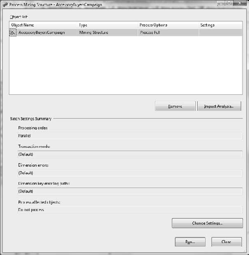
When the Process Progress dialog box appears and the Status area displays Process Succeeded, click Close. This returns you to the Process Mining Structure dialog box. Click Close again.
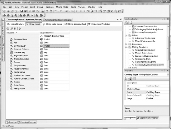
With our processing complete, you can now explore the other tabs. Click the Mining Models tab, as shown in Figure 11-11. In this view, you can review your Structure Mining columns and Mining Model columns. Also notice that your mining model name is shown at the top of the Mining Model columns. Update both the Accessory Buyer and Clothing Buyer to Predict from PredictOnly.
Next, process the model to reflect our Buyer column changes. When this completes, click the Mining Model Viewer tab.
The Mining Model Viewer is a container that supports several viewers. Choosing Microsoft Tree Viewer from the Viewer drop-down will load your Accessory Buyers campaign into the Tree Viewer. After the Tree Viewer has loaded, ensure that Accessory Buyer is selected in the Tree drop-down, which is just below the Viewer drop-down list. In this section, I will show you the Microsoft Tree Viewer, the Mining Legend, and this model's drill-through capability.
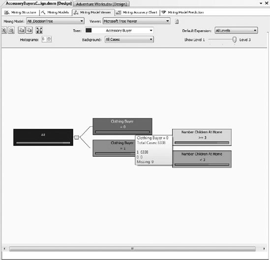
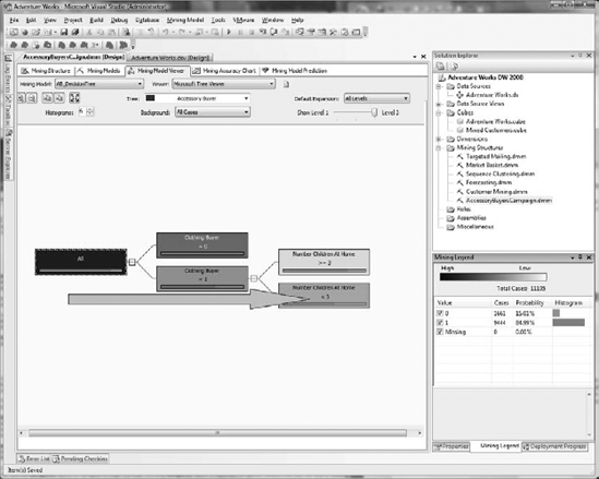
The decision tree is built as a series of splits, from left to right, as shown in Figure 11-12. The leftmost node is All, which represents the entire campaign. The background color of each node is an indication of that node's population; the darker the color, the greater the population.
In your model, All is the darkest. To the right of All, the Clothing Buyer = 0 node is larger than Clothing Buyer = 1. If you hover over Clothing Buyer = 0, an infotip will show the size of this node as 6,338. Doing this on the Clothing Buyer = 1 node will display 4,767.
Each node in the bar under the node condition is a histogram that represents our buyers. The blue portion of the bar is our True state, and the pink our False state. Click the All node and select Show Legend. After the legend appears, dock it in the lower-right corner, as shown in Figure 11-13. Doing this makes it easier to watch the values as you navigate the tree.
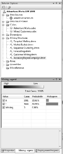
The Mining Legend has four columns of information about your model. The first column, Value, shows 0, 1, and Missing. 0 is our false, or nonbuyer case, while 1 is our true, or buyer case. The Missing value of 0 is good to see, as it indicates that our data is clean and fully populated. Our Cases column displays the population of each case, and the Probability calculates this distribution as a percentage. Finally, the Histogram column mimics the node's histogram.
Reading the decision tree is done in a left-to-right manner, as shown in Figure 11-14. In our Accessory Buyer model, the most significant factor that determines our accessory buyers is whether they are also clothing buyers. This factor alone can enable the creation of a focused campaign. But in our case, we see another valuable factor is at work here. The Number Children At Home node contains some interesting values. The Number Children At Home >= 3 has a higher probability of purchase per its histogram than the Number Children At Home < 3. On the other hand, the Number Children At Home < 3 is a darker node, meaning it has a greater population. Let's take a closer look.
Click the Number Children At Home >= 3 node and review the Mining Legend. Our accessory buyers equal 722, with a probability of 78.52 percent. Reviewing the Number Children At Home < 3 reveals 2,384 cases, with a probability of 61.95 percent. Based on these figures, your marketing group may decide to target the group with fewer than three children at home first, because it has more buyers.
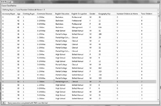
Using drill-through, which you enabled when creating the AccessoryBuyers mining model, enables you to see the underlying data that belongs to a particular node. Right-click the Number Children At Home < 3 node and select Drill Through, followed by Model Columns Only.
The Drill Through grid, shown in Figure 11-15, displays your training cases classified to Clothing Buyer = 1 and Number Children At Home < 3. The model's data points are displayed in alphabetical order (I've hidden a few to narrow the view). Take note of the Number Children At Home column. It contains values of 0, 1, and 2. This Number Children At Home bucket was created by the Decision Tree algorithm during model processing.
Tip
If you right-click on the grid contents and select Copy All, a copy of your cases will be placed into the copy buffer, complete with column headings. This data can then be pasted into an Excel worksheet for further analysis.
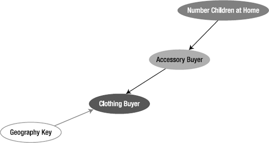
You use the Dependency Network to view the input/predictable attribute dependencies in your model. Clicking the Number Children At Home node will change the node display in the following ways:
- Selected node:
The background color will change to turquoise.
- Predicts this node:
If the selected node predicts this node, this node's background color will change to a slate-blue.
Next, click the Clothing Buyer node. Choosing Clothing Buyer will change the Dependency Network view in the following ways:
Finally, select the Accessory Buyer node, right-click, and select Copy Graph View. This copies your Dependency Network, shown in Figure 11-16, to the Windows Clipboard.
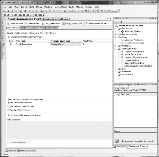
The Mining Accuracy Chart tab, shown in Figure 11-17, is where you will validate your mining models. For your Decision Tree model, you will be using the Input Selection and Lift Chart tabs. In the Input Selection tab's Predictable Column Name column, select Accessory Buyer. After this, select 1 for Predict Value. From the Select Data Set to be Used for Accuracy Chart section, confirm that Use Mining Model Test Cases is selected.
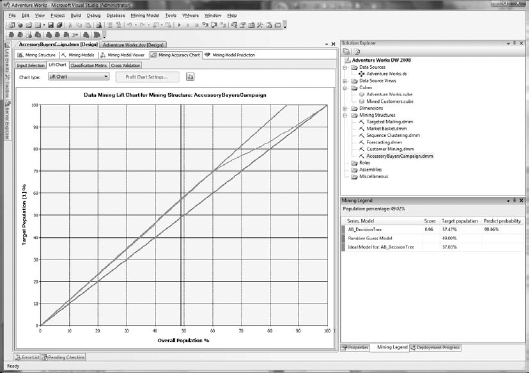
With the Input Selection tab completed, choose the Lift Chart tab. After a moment of processing, the Data Mining Lift Chart for Mining Structure: AccessoryBuyersCampaign, and the Mining Legend that you docked earlier will appear.
The lift chart, shown in Figure 11-18, will help you determine the value of your model. The lift chart evaluates and compares your targets by using an ideal line and a random line. The percentage amount difference between your lift line and your random line is referred to as lift in the marketing world. The lift chart lines are defined as follows:
- Random line:
The random line is drawn as a straight diagonal line, from (0, 0) to (100, 100). For a mining model to be considered a productive model, it should show some lift above this baseline.
- Ideal line:
Shown in green for this model this line reaches 100 percent Overall Population at 85 percent Target Population. The ideal line for the Accessory Buyers campaign suggests that a perfectly constructed model would reach 100 percent of your targets by using only 85 percent of the target population.
- Lift line:
This coral-colored line represents your model. The Accessory Buyers campaign follows the ideal line for quite a ways, meaning that our model is performing quite well. Deciding to contact more than 60 percent of the overall population will be a discussion point with marketing, because this is where your model begins to trend back toward the random line.
- Measured location line:
This is the vertical gray line in the middle of the chart. This line can be moved simply by clicking inside the chart. Moving this line will automatically update the Mining Legend with the appropriate values.
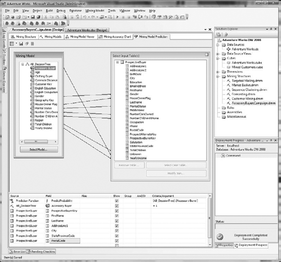
Now you are ready to create a prediction. Selecting the Mining Model Prediction tab displays the Prediction Query Builder in Design view. Initially, there will be no selections in the Select Input Tables(s) area, or in the Source/Field grid at the bottom of the designer.
To create your prediction query, complete the following steps:
Select a mining model: if AB_DecisionTree is not loaded in the Mining Model box, click the Select Model button to navigate your data models. Expand the AccessoryBuyersCampaign, and choose the AB_DecisionTree model.
Select your input table: in the Select Input Table(s) box, click the Select Case Table button. In the Select Table dialog box, pick AccessoryCampaign from the Data Source drop-down. After you have done this, choose the ProspectiveBuyer table that marketing purchased, and click OK. Notice that seven fields are automatically mapped between the mining model and the ProspectiveBuyer table.
Map columns: in addition to the preceding columns that were mapped automatically, we need to add our predict column. To do this, simply drag and drop the Accessory Buyer column in your mining model onto the Unknown column in the input table.
Design the query: In the Source/Field grid, you will select the specific data points and data types to output for your prediction. Begin by choosing Prediction Function from the Source drop-down list. In the Field drop-down list, select PredictProbability. The last thing needed for our prediction function is to drag and drop the Accessory Buyer column from the mining model to the Criteria/Argument cell. Doing this will replace the cell's text with
[AB_DecisionTree].[Accessory Buyer]. Next, you will add another row to the grid. Choose AB_DecisionTree from the drop-down list in the row below Prediction Function. In the Field column, ensure that Accessory Buyer is chosen. You want to predict who your future buyers may be, so enter = 1 in the Criteria/Argument column. Finally, you will want to identify your possible customers. Do this by selecting ProspectiveBuyer in the next Source column, and ProspectiveBuyerKey in the Field column.Add other prospect information: Add additional customer information to the grid by creating six new rows. For the first row, select ProspectiveBuyer as your source, followed by FirstName as your field. Repeat the preceding steps five more times, adding LastName, AddressLine1, City, StateProvinceCode, and PostalCode.
When you have completed these steps, your Mining Model Prediction view should look like Figure 11-19.
It is now time to run the prediction and view our results. Click the Switch to Query Result View (leftmost) button in this tab's toolbar. Your prediction query will process, and you will be presented with a grid, shown in Figure 11-20, containing your accessory buying targets.
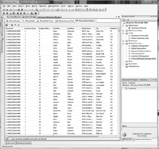
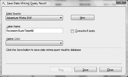
These targets can be saved to your database by clicking the Save Query Result button (second from the left), which is also in this tab's toolbar. In the Save Data Mining Query Result dialog box, Select Adventure Works DW from the Data Source drop-down. Enter AccessoryBuyerTargets as your table name, as shown in Figure 11-21, and click Save.
It's time to turn our attention to Microsoft Data Mining Extensions (DMX). DMX, as a query language, has a syntax that is quite similar to Transact-SQL (T-SQL). In this section of the chapter, you will use DMX to create, train, and explore the Accessory Buyers campaign with the Microsoft Naïve Bayes algorithm.
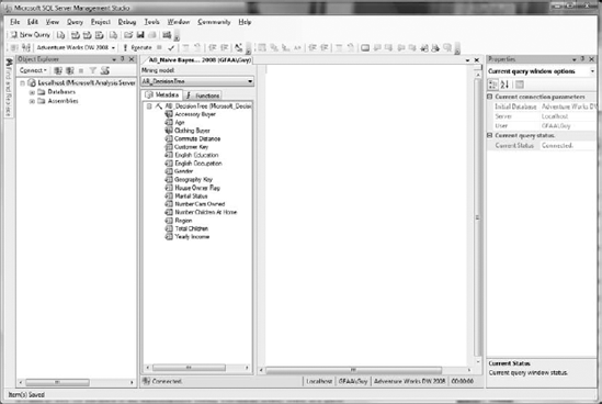
To ready your development environment to create the DMX queries, launch SQL Server Management Studio (SSMS). In the Connect to Server dialog box, select Analysis Services from the Server Type drop-down list. Choose or enter your Server Name and Authentication information, and click Connect. Right-click the Analysis Services (SSAS) instance you just connected to, point to New Query, and click DMX. Figure 11-22 displays a new DMX query window.
Your first task will be to drop the existing AccessoryBuyersCampaign mining structure. To do this, simply enter the following code into the query window, and click Execute in the toolbar:
--Drop structure, if needed
Drop Mining Structure AccessoryBuyersCampaign;
The next step is to create the AccessoryBuyersCampaign mining structure using DMX. Enter the following code into the query window, highlight it, and click Execute:
--Create AccessoryBuyersCampaign mining structure
Create Mining Structure [AccessoryBuyersCampaign]
(
   [Customer Key]             Long     Key,
   [Accessory Buyer]          Long     Discrete,
   [Age]                      Long     Discretized(Automatic, 10),
   [Commute Distance]         Text     Discrete,
   [English Education]        Text     Discrete,
   [English Occupation]       Text     Discrete,
   [Gender]                   Text     Discrete,
[House Owner Flag]         Text     Discrete,
   [Marital Status]           Text     Discrete,
   [Number Cars Owned]        Long     Discrete,
   [Number Children At Home]  Long     Discrete,
   [Region]                   Text     Discrete,
   [Yearly Income]            Double   Discretized(Automatic, 10)
)
With Holdout (30 Percent);
In the preceding code, you can see the similarity of syntax in DMX and T-SQL. The holdout of 30 percent is what you entered in the Create Testing Set earlier in this chapter. Note the Discretized(Automatic, 10) content type. In this statement, you are stating that you want the algorithm to automatically create ten buckets. It is common to start with ten buckets when creating new structures.
Now that your mining structure is in place, you can use DMX to create mining models. Use the following code to add a Naïve Bayes model to the mining structure you have created:
--Add a Naive Bayes model for the Accessory Buyers Campaign
Alter Mining   Structure   AccessoryBuyersCampaign
Add   Mining   Model       AB_NaiveBayes
(
   [Customer Key],
   [Accessory Buyer]       Predict,

   [Age],
   [Commute Distance],
   [English Education],
   [English Occupation],
   [Gender],
   [House Owner Flag],
   [Marital Status],
   [Number Cars Owned],
   [Number Children At Home],
   [Region],
   [Yearly Income]
)
Using Microsoft_Naive_Bayes;
In the preceding code, you added the AB_NaiveBayes model to the AccessoryBuyersCampaign mining structure. Note the explicit assignment of Accessory Buyer for prediction.
Now that you have successfully created a mining structure and added a model to it, it is time to process the Accessory Buyers campaign. To process this structure, enter the following code and execute it:
--Process the Accessory Buyer mining structure
Insert Into Mining Structure AccessoryBuyersCampaign
(
   [Customer Key],
   [Accessory Buyer],

   [Age],
   [Commute Distance],
   [English Education],
   [English Occupation],
   [Gender],
   [House Owner Flag],
   [Marital Status],
   [Number Cars Owned],
   [Number Children At Home],
   [Region],
   [Yearly Income])
OpenQuery
(
   [Adventure Works DW],
   'SELECT
      CustomerKey,
      AccessoryBuyer,
      Age,
      CommuteDistance,
      EnglishEducation,
      EnglishOccupation,
      Gender,
      HouseOwnerFlag,
      MaritalStatus,
      NumberCarsOwned,
      NumberChildrenAtHome,
      Region,
      YearlyIncome
    FROM
      dbo.vAccessoryBuyers'
);To view the Accessory Buyers mining model, you use a variant of the standard T-SQL Select statement. The main difference here is that instead of viewing data from a table, you view the content of a mining model. Enter the following into a query window and execute it:
Select   Distinct   [Age]
From     AB_NaiveBayes
This simple query will return the distinct ages in your model. This is useful for discretized columns, as the returned data set represents the buckets chosen by the algorithm.
Age
32
38
44
48
53
59
64
68
74
81
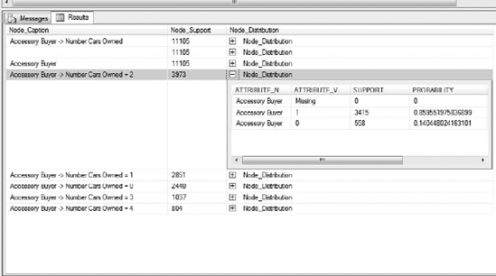
This next DMX query will look at the decisions made by the algorithm. Note that the mining columns listed are not defined in your mining structure. These columns are added during model processing to hold values calculated by the model. The Node_Caption column contains the name of each node, while the Node_Support column displays the number of cases belonging to the node. The Node_Distribution column is expandable, and contains the same data as the mining legend.
Enter the next query and execute it:
--Review node data in this model
Select
   Node_Caption,
   Node_Support,
   Node_Distribution
From
   AB_NaiveBayes.Content
Where
   Node_Support > 0
Order By
   Node_Support Desc
After executing the preceding query, the Results grid shown in Figure 11-23 will display your data.
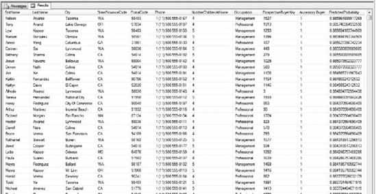
The final product is at hand! It's now time to predict your accessory buyers. To do this, you will create and execute a DMX query that joins your mining model to your prospective buyers. This type of join is called a Prediction Join, and uses the same OpenQuery syntax you used in the processing section. Note the PredictProbability call to Accessory Buyer, which returns the probability of this target being an accessory buyer. The following query returns our predicted buyers:
--Predict our Accessory Buyers
Select
   PB.FirstName,
   PB.LastName,
   PB.City,
   PB.StateProvinceCode,
   PB.PostalCode,
   PB.Phone,
   PB.NumberChildrenAtHome,
   PB.Occupation,
   PB.ProspectiveBuyerKey,
   AB_NaiveBayes.[Accessory Buyer],
   PredictProbability([Accessory Buyer]) As PredictedProbability
From
   AB_NaiveBayes
Prediction Join
   OpenQuery
   (
[Adventure Works DW],
      'SELECT
         ProspectiveBuyerKey,
         FirstName,
         LastName,
         City,
         StateProvinceCode,
         PostalCode,
         Education,
         Occupation,
         Phone,
         HouseOwnerFlag,
         NumberCarsOwned,
         NumberChildrenAtHome,
         MaritalStatus,
         Gender,
         YearlyIncome
      FROM
         dbo.ProspectiveBuyer'
   ) As PB
On
   AB_NaiveBayes.[Marital Status] = PB.[MaritalStatus] And
   AB_NaiveBayes.[Gender] = PB.[Gender] And
   AB_NaiveBayes.[Yearly Income] = PB.[YearlyIncome] And
   AB_NaiveBayes.[Number Children At Home] = PB.[NumberChildrenAtHome] And
   AB_NaiveBayes.[English Education] = PB.[Education] And
   AB_NaiveBayes.[English Occupation] = PB.[Occupation] And
   AB_NaiveBayes.[House Owner Flag] = PB.[HouseOwnerFlag] And
   AB_NaiveBayes.[Number Cars Owned] = PB.[NumberCarsOwned]
Where
   AB_NaiveBayes.[Accessory Buyer] = 1
Order By
   PredictProbability([Accessory Buyer]) Desc;
Enter this query into your query window and execute it. A portion of the predicted accessory buyers, per Naïve Bayes, appears in Figure 11-24.
This chapter began by making a case for data mining as an integral part of any business intelligence effort. After reviewing a few of the more common algorithms, we delved into the Accessory Buyer marketing campaign. Using Analysis Services and the Business Intelligence Development Studio, you created a mining model, validated your model, and predicted future customers by using Microsoft Decision Trees.
In the next section, you used DMX to create, validate, and predict future accessory buyers—only this time, you did so in SQL Server Management Studio, using a query-only approach. Now you will move on to PowerPivot, where you will use Excel to work with multidimensional data from your desktop.