![]()
R Language Primer
In the last chapter, we defined what data visualizations are, looked at a little bit of the history of the medium, and explored the process for creating them. This chapter takes a deeper dive into one of the most important tools for creating data visualizations: R.
When creating data visualizations, R is an integral tool for both analyzing data and creating visualizations. We will use R extensively through the rest of this book, so we had better level set first.
R is both an environment and a language to run statistical computations and produce data graphics. It was created by Ross Ihaka and Robert Gentleman in 1993 while at University of Auckland. The R environment is the runtime environment that you develop and run R in. The R language is the programming language that you develop in.
R is the successor to the S language, a statistical programming language that came out of Bell Labs in 1976.
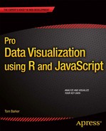
Let’s start by downloading and installing R. R is available from the R Foundation at http://www.r-project.org/. See Figure 2-1 for a screenshot of the R Foundation homepage.
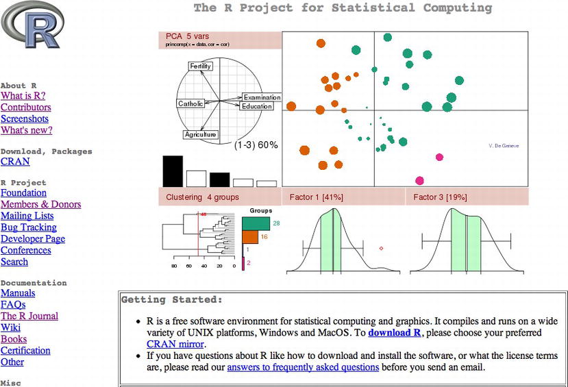
Figure 2-1. Homepage of the R Foundation
It is available as a precompiled binary from the Comprehensive R Archive Network (CRAN) website: http://cran.r-project.org/ (see Figure 2-2). We just select our operating system and what version of R we want, and we can begin to download.
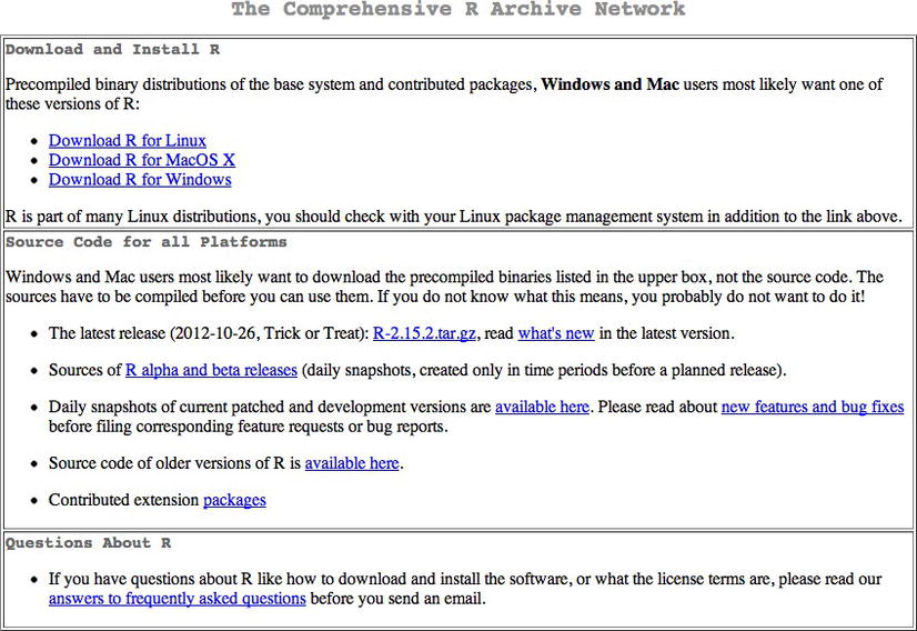
Figure 2-2. The CRAN website
Once the download is complete, we can run through the installer. See Figure 2-3 for a screenshot of the R installer for the Mac OS.
Figure 2-3. R installation on a Mac
Once we finish the installation we can launch the R application, and we are presented with the R console, as shown in Figure 2-4.
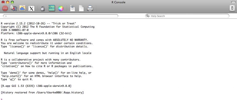
Figure 2-4. The R console
The Command Line
The R console is where the magic happens! It is a command-line environment where we can run R expressions. The best way to get up to speed in R is to script in the console, a piece at a time, generally to try out what you’re trying to do, and tweak it until you get the results that you want. When you finally have a working example, take the code that does what you want and save it as an R script file.
R script files are just files that contain pure R and can be run in the console using the source command:
> source("someRfile.R")
Looking at the preceding code snippet, we assume that the R script lives in the current work directory. The way we can see what the current work directory is to use the getwd() function:
> getwd()
[1] "/Users/tomjbarker"
We can also set the working directory by using the setwd() function. Note that changes made to the working directory are not persisted across R sessions unless the session is saved.
> setwd("/Users/tomjbarker/Downloads")
> getwd()
[1] "/Users/tomjbarker/Downloads"
Command History
The R console stores commands that you enter and you can cycle through previous commands by pressing the up arrow. Hit the escape button to return to the command prompt. We can see the history in a separate window pane by clicking the Show/Hide Command History button at the top of the console. The Show/Hide Command History button is the rectangle icon with alternating stripes of yellow and green. See Figure 2-5 for the R console with the command history shown.
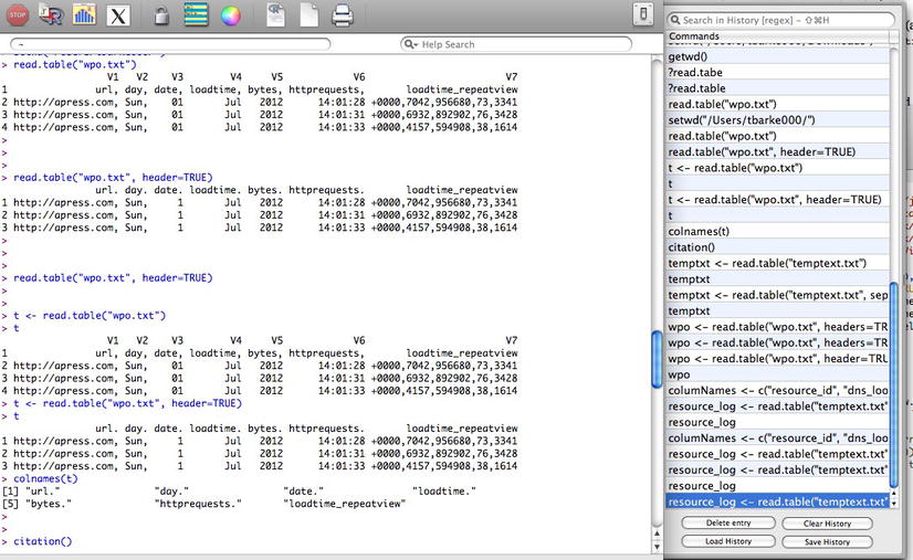
Figure 2-5. R console with command history shown
Accessing Documentation
To read the R documentation around a specific function or keyword, you simply type a question mark before the keyword:
> ?setwd
If you want to search the documentation for a specific word or phrase, you can type two question marks before the search query:
> ??"working directory"
This code launches a window that shows search results (see Figure 2-6). The search result window has a row for each topic that contains the search phrase and has the name of the help topic, the package that the functionality that the help topic talks about is in, and a short description for the help topic.
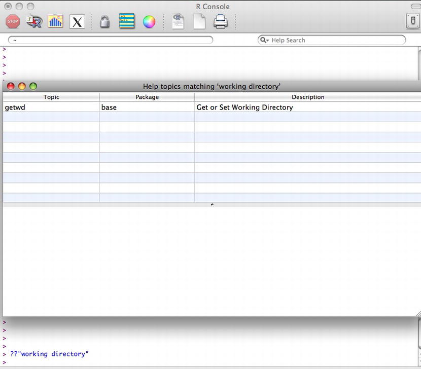
Figure 2-6. Help search results window
Packages
Speaking of packages, what are they, exactly? Packages are collections of functions, data sets, or objects that can be imported into the current session or workspace to extend what we can do in R. Anyone can make a package and distribute it.
To install a package, we simply type this:
install.packages([package name])
For example, if we want to install the ggplot2 package—which is a widely used and very handy charting package—we simply type this into the console:
> install.packages("ggplot2")
We are immediately prompted to choose the mirror location that we want to use, usually the one closest to our current location. From there, the install begins. We can see the results in Figure 2-7.
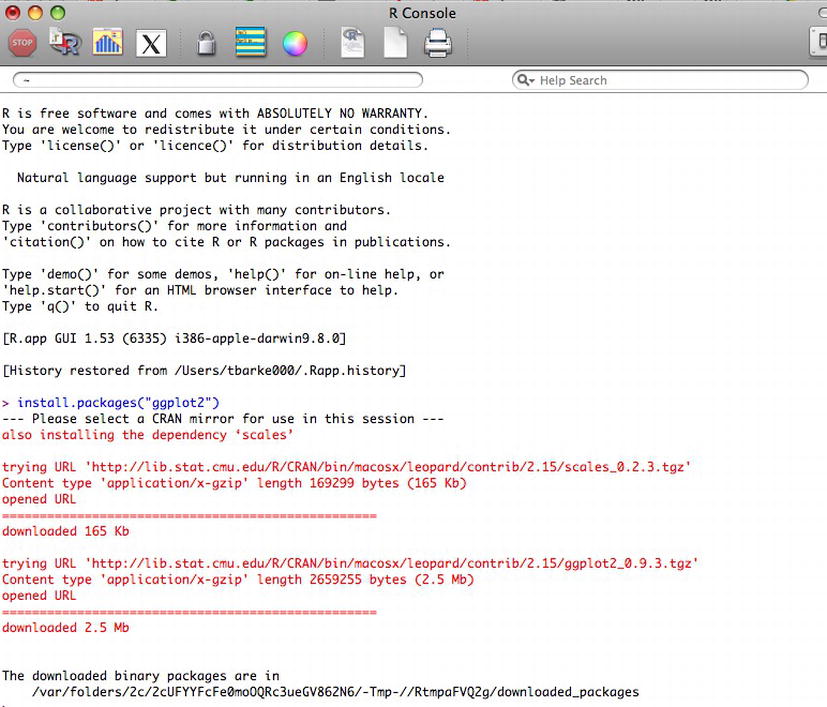
Figure 2-7. Installing the ggplot2 package
The zipped-up package is downloaded and exploded into our R installation.
If want to use a package that we have installed, we must first include it in our workspace. To do this we use the library() function:
> library(ggplot2)
A list of packages available at the CRAN can be found here: http://cran.r-project.org/web/packages/available_packages_by_name.html.
To see a list of packages already installed, we can simply call the library() function with no parameter (depending on your install and your environment, your list of packages may vary):
> library()
Packages in library '/Library/Frameworks/R.framework/Versions/2.15/Resources/library':
barcode                         Barcode distribution plots
base                            The R Base Package
boot                            Bootstrap Functions (originally by Angelo Canty for S)
class                           Functions for Classification
cluster                         Cluster Analysis Extended Rousseeuw et al.
codetools                       Code Analysis Tools for R
colorspace                      Color Space Manipulation
compiler                        The R Compiler Package
datasets                        The R Datasets Package
dichromat                       Color schemes for dichromats
digest                          Create cryptographic hash digests of R objects
foreign                         Read Data Stored by Minitab, S, SAS, SPSS, Stata, Systat, dBase,
                               ...
ggplot2                         An implementation of the Grammar of Graphics
gpairs                          gpairs: The Generalized Pairs Plot
graphics                        The R Graphics Package
grDevices                       The R Graphics Devices and Support for Colours and Fonts
grid                            The Grid Graphics Package
gtable                          Arrange grobs in tables.
KernSmooth                      Functions for kernel smoothing for Wand & Jones (1995)
labeling                        Axis Labeling
lattice                         Lattice Graphics
mapdata                         Extra Map Databases
mapproj                         Map Projections
maps                            Draw Geographical Maps
Importing Data
So now our environment is downloaded and installed, and we know how to install any packages that we may need. Now we can begin using R.
The first thing we’ll normally want to do is import your data. There are several ways to import data, but the most common way is to use the read() function, which has several flavors:
read.table("[file to read]")
read.csv(["file to read"])
To see this in action, let’s first create a text file named temptext.txt that is formatted like so:
134,432,435,313,11
403,200,500,404,33
77,321,90,2002,395
We can read this into a variable that we will name temptxt:
> temptxt <- read.table("temptext.txt")
Notice that as we are assigning value to this variable, we are not using an equal sign as the assignment operator. We are instead using an arrow <-. That is R’s assignment operator, although it does also support the equal sign if you are so inclined. But the standard is the arrow, and all examples that we will show in this book will use the arrow.
If we print out the temptxt variable, we see that it is structured as follows:
> temptxt
                 V1
1 134,432,435,313,11
2 403,200,500,404,33
3 77,321,90,2002,395
We see that our variable is a table-like structure called a data frame, and R has assigned a column name (V1) and row IDs to our data structure. More on column names soon.
The read() function has a number of parameters that you can use to refine how the data is imported and formatted once it is imported.
Using Headers
The header parameter tells R to treat the first line in the external file as containing header information. The first line then becomes the column names of the data frame.
For example, suppose we have a log file structured like this:
url, day, date, loadtime, bytes, httprequests, loadtime_repeatview
http://apress.com, Sun, 01 Jul 2012 14:01:28 +0000,7042,956680,73,3341
http://apress.com, Sun, 01 Jul 2012 14:01:31 +0000,6932,892902,76,3428
http://apress.com, Sun, 01 Jul 2012 14:01:33 +0000,4157,594908,38,1614
We can load it into a variable named wpo like so:
> wpo <- read.table("wpo.txt",header=TRUE)
> wpo
  url  day date loadtime bytes httprequests loadtime_repeatview
1 http://apress.com,Sun,1 Jul 2012 14:01:28 +0000,7042,955550,73,3191
2 http://apress.com,Sun,1 Jul 2012 14:01:31 +0000,6932,892442,76,3728
3 http://apress.com,Sun,1 Jul 2012 14:01:33 +0000,4157,614908,38,1514
When we call the colnames() function to see what the column names are for wpo, we see the following:
> colnames(wpo)
[1] "url"     "day"     "date"     "loadtime"
[5] "bytes"     "httprequests"     "loadtime_repeatview"
Specifying a String Delimiter
The sep attribute tells the read() function what to use as the string delimiter for parsing the columns in the external data file. In all the examples we’ve looked at so far, commas are our delimiters, but we could use instead pipes | or any other character that we want.
Say, for example, that our previous temptxt example used pipes; we would just update the code to be as follows:
134|432|435|313|11
403|200|500|404|33
77|321|90|2002|395

> temptxt <- read.table("temptext.txt",sep="|")
> temptxt
  V1  V2  V3   V4  V5
1 134 432 435  313  11
2 403 200 500  404  33
3  77 321  90 2002 395
Oh, notice that? We actually got distinct column names this time (V1, V2, V3, V4, V5). Before, we didn’t specify a delimiter, so R assumed that each row was one big blob of text and lumped it into a single column (V1).
Specifying Row Identifiers
The row.names attribute allows us to specify identifiers for our rows. By default, as we’ve seen in the previous examples, R uses incrementing numbers as row IDs. Keep in mind that the row names need to be unique for each row.
With that in mind, let’s take a look at importing some different log data, which has performance metrics for unique URLs:
url, day, date, loadtime, bytes, httprequests, loadtime_repeatview
http://apress.com, Sun, 01 Jul 2012 14:01:28 +0000,7042,956680,73,3341
http://google.com, Sun, 01 Jul 2012 14:01:31 +0000,6932,892902,76,3428
http://apple.com, Sun, 01 Jul 2012 14:01:33 +0000,4157,594908,38,1614
When we read it in, we’ll be sure to specify that the data in the url column should be used as the row name for the data frame.
> wpo <- read.table("wpo.txt", header=TRUE, sep=",", row.names="url")
> wpo
                  day                        date loadtime  bytes httprequests loadtime_repeatview
http://apress.com  Sun  01 Jul 2012 14:01:28 +0000     7042 956680           73                3341
http://google.com  Sun  01 Jul 2012 14:01:31 +0000     6932 892902           76                3428
http://apple.com   Sun  01 Jul 2012 14:01:33 +0000     4157 594908           38                1614
Using Custom Column Names
And there we go. But what if we want to have column names, but the first line in our file is not header information? We can use the col.names parameter to specify a vector that we can use as column names.
Let’s take a look. In this example, we’ll use the pipe separated text file used previously.
134|432|435|313|11
403|200|500|404|33
77|321|90|2002|395
First, we’ll create a vector named columnNames that will hold the strings that we will use as the column names:
> columnNames <- c("resource_id", "dns_lookup", "cache_load", "file_size", "server_response")
Then we’ll read in the data, passing in our vector to the col.names parameter.
> resource_log <- read.table("temptext.txt", sep="|", col.names=columnNames)
> resource_log
 resource_id dns_lookup cache_load file_size server_response
1         134        432        435       313              11
2         403        200        500       404              33
3          77        321         90      2002             395
Data Structures and Data Types
In the previous examples, we touched on a lot of concepts; we created variables, including vectors and data frames; but we didn’t talk much about what they are. Let’s take a step back and look at the data types that R supports and how to use them.
Data types in R are called modes, and can be the following:
- numeric
- character
- logical
- complex
- raw
- list
We can use the mode() function to check the mode of a variable.
Character and numeric modes correspond to string and number (both integer and float) data types. Logical modes are Boolean values.
> n <- 122132
> mode(n)
[1] "numeric"
> c <- "test text"
> mode(c)
[1] "character"
> l <- TRUE
> mode(l)
[1] "logical"
We can perform string concatenation using the paste() function. We can use the substr() function to pull characters out of strings. Let’s look at some examples in code.
Usually, I keep a list of directories that I either read data from or write charts to. Then when I want to reference a new data file that exists in the data directory, I will just append the new file name to the data directory:
> dataDirectory <- "/Users/tomjbarker/org/data/"
> buglist <- paste(dataDirectory, "bugs.txt", sep="")
> buglist
[1] "/Users/tomjbarker/org/data/bugs.txt"
The paste() function takes N amount of strings and concatenates them together. It accepts an argument named sep that allows us to specify a string that we can use to be a delimiter between joined strings. We don’t want anything separating our joined strings that we pass in an empty string.
If we want to pull characters from a string, we use the substr() function. The substr() function takes a string to parse, a starting location, and a stopping location. It returns all the character inclusively from the starting location up to the ending location. (Remember that in R, lists are not 0-based like most other languages, but instead have a starting index of 1.)
> substr("test", 1,2)
[1] "te"
In the preceding example, we pass in the string “test” and tell the substr() function to return the first and second characters.
Complex mode is for complex numbers. The raw mode is to store raw byte data.
List data types or modes can be one of three classes: vectors, matrices, or data frames. If we call mode() for vectors or matrices, they return the mode of the data that they contain; class() returns the class. If we call mode() on a data frame, it returns the type list:
> v <- c(1:10)
> mode(v)
[1] "numeric"
> m <- matrix(c(1:10), byrow=TRUE)
> mode(m)
[1] "numeric"
> class(m)
[1] "matrix"
> d <- data.frame(c(1:10))
> mode(d)
[1] "list"
> class(d)
[1] "data.frame"
Note that we just typed 1:10 rather than the whole sequence of numbers between 1 and 10:
v <- c(1:10)
Vectors are single-dimensional arrays that can hold only values of a single mode at a time. It’s when we get to data frames and matrices that R really starts to get interesting. The next two sections cover those classes.
Data Frames
We saw at the beginning of this chapter that the read() function takes in external data and saves it as a data frame. Data frames are like arrays in most other loosely typed languages: they are containers that hold different types of data, referenced by index. The main thing to realize, though, is that data frames see the data that they contain as rows, columns, and combinations of the two.
For example, think of a data frame as formatted as follows:
      col  col  col  col  col
row [ 1 ] [ 1 ] [ 1 ] [ 1 ] [ 1 ]
row [ 1 ] [ 1 ] [ 1 ] [ 1 ] [ 1 ]
row [ 1 ] [ 1 ] [ 1 ] [ 1 ] [ 1 ]
row [ 1 ] [ 1 ] [ 1 ] [ 1 ] [ 1 ]
If we try to reference the first index in the preceding data frame as we traditionally would with an array, say dataframe[1], R would instead return the first column of data, not the first item. So data frames are referenced by their column and row. So dataframe[1] returns the first column and dataframe[,2] returns the first row.
Let’s demonstrate this in code.
First let’s create some vectors using the combine function, c(). Remember that vectors are collections of data all of the same type. The combine function takes a series of values and combines them into vectors.
> col1 <- c(1,2,3,4,5,6,7,8)
> col2 <- c(1,2,3,4,5,6,7,8)
> col3 <- c(1,2,3,4,5,6,7,8)
> col4 <- c(1,2,3,4,5,6,7,8)
Then let’s combine these vectors into a data frame:
> df <- data.frame(col1,col2,col3,col4)
Now let’s print the data frame to see the contents and the structure of it:
> df
    col1 col2 col3 col4
1    1    1    1    1
2    2    2    2    2
3    3    3    3    3
4    4    4    4    4
5    5    5    5    5
6    6    6    6    6
7    7    7    7    7
8    8    8    8    8
Notice that it took each vector and made each one a column. Also notice that each row has an ID; by default, it is a number, but we can override that.
If we reference the first index, we see that the data frame returns the first column:
> df[1]
 col1
1    1
2    2
3    3
4    4
5    5
6    6
7    7
8    8
If we put a comma in front of that 1, we reference the first row:
> df[,1]
[1] 1 2 3 4 5 6 7 8
So accessing contents of a data frame is done by specifying [column, row].
Matrices work much the same way.
Matrices
Matrices are just like data frames in that they contain rows and columns and can be referenced by either. The core difference between the two is that data frames can hold different data types but matrices can hold only one type of data.
This presents a philosophical difference. Usually you use data frames to hold data read in externally, like from a flat file or a database because those are generally of mixed type. You normally store data in matrices that you want to apply functions to (more on applying functions to lists in a little bit).
To create a matrix, we must use the matrix() function, pass in a vector, and tell the function how to distribute the vector:
- The nrow parameter specifies how many rows the matrix should have
- The ncol parameter specifies the number of columns.
- The byrow parameter tells R that the contents of the vector should be distributed by iterating across rows if TRUE or by columns if FALSE.
> content <- c(1,2,3,4,5,6,7,8,9,10)
> m1 <- matrix(content, nrow=2, ncol=5, byrow=TRUE)
> m1
    [,1] [,2] [,3] [,4] [,5]
[1,]    1    2    3    4    5
[2,]    6    7    8    9   10
>
Notice that in the previous example that the m1 matrix is filled in horizontally, row by row. In the following example, the m1 matrix is filled in vertically by column:
> content <- c(1,2,3,4,5,6,7,8,9,10)
> m1 <- matrix(content, nrow=2, ncol=5, byrow=FALSE)
> m1
    [,1] [,2] [,3] [,4] [,5]
[1,]    1    3    5    7    9
[2,]    2    4    6    8   10
Remember that instead of manually typing out all the numbers in the previous content vector, if the numbers are a sequence we can just type this:
content <- (1:10)
We reference the content in matrices with the square bracket, specifying the row and column, respectively.
> m1[1,4]
[1] 7
We can convert a data frame to a matrix if the data frame contains only a single type of data. To do this we use the as.matrix() function. Often times we will do this when passing a data frame to a plotting function to draw a chart.
> barplot(as.matrix(df))
Below we create a data frame called df. We populate the data frame with ten consecutive numbers. We then use as.matrix() to convert df into a matrix and save the result into a new variable called m:
> df <- data.frame(1:10)
> df
  X1.10
1      1
2      2
3      3
4      4
5      5
6      6
7      7
8      8
9      9
10    10
> class(df)
[1] "data.frame"
> m <- as.matrix(df)
> class(m)
[1] "matrix"
Keep in mind that because they are all the same data type, matrices require less overhead and are intrinsically more efficient than data frames. If we compare the size of our matrix m and our data frame df, we see that with just ten items there is a size difference.
> object.size(m)
312 bytes
> object.size(df)
440 bytes
With that said, if we increase the scale of this, the increase in efficiency does not equally scale. Compare the following:
> big_df <- data.frame(1:40000000)
> big_m <- matrix(1:40000000)
> object.size(big_m)
160000112 bytes
> object.size(big_df)
160000400 bytes
We can see that the first example with the small data set showed that the matrix was 30 percent smaller in size than the data frame, but at the larger scale in the second example the matrix was only .00018 percent smaller than the data frame.
Adding Lists
When combining or adding to data frames or matrices, you generally add either by the row or the column using rbind() or cbind().
To demonstrate this, let’s add a new row to our data frame df. We’ll pass df into rbind() along with the new row to add to df. The new row contains just one element, the number 11:
> df <- rbind(df, 11)
> df
  X1.10
1      1
2      2
3      3
4      4
5      5
6      6
7      7
8      8
9      9
10    10
11    11
Now let’s add a new column to our matrix m. To do this, we simply pass m into cbind() as the first parameter; the second parameter is a new matrix that will be appended to the new column.
> m <- rbind(m, 11)
> m <- cbind(m, matrix(c(50:60), byrow=FALSE))
> m
     X1.10
[1,]     1 50
[2,]     2 51
[3,]     3 52
[4,]     4 53
[5,]     5 54
[6,]     6 55
[7,]     7 56
[8,]     8 57
[9,]     9 58
[10,]    10 59
[11,]    11 60
What about vectors, you may ask? Well, let’s look at adding to our content vector. We simply use the combine function to combine the current vector with a new vector:
> content <- c(1,2,3,4,5,6,7,8,9,10)
> content <- c(content, c(11:20))
> content
[1]  1  2  3  4  5  6  7  8  9 10 11 12 13 14 15 16 17 18 19 20
Looping Through Lists
As developers who generally work in procedural languages, or at least came up the ranks using procedural languages (though in recent years functional programming paradigms have become much more mainstream), we’re most likely used to looping through our arrays when we want to process the data within them. This is in contrast to purely functional languages where we would instead apply a function to our lists, like the map() function. R supports both paradigms. Let’s first look at how to loop through our lists.
The most useful loop that R supports is the for in loop. The basic structure of a for in loop can be seen here:.
> for(i in 1:5){print(i)}
[1] 1
[1] 2
[1] 3
[1] 4
[1] 5
The variable i increments in value each step through the iteration. We can use the for in loop to step through lists. We can specify a particular column to iterate through, like the following, in which we loop through the X1.10 column of the data frame df.
> for(n in df$X1.10){ print(n)}
[1] 1
[1] 2
[1] 3
[1] 4
[1] 5
[1] 6
[1] 7
[1] 8
[1] 9
[1] 10
[1] 11
Note that we are accessing the columns of data frames via the dollar sign operator. The general pattern is [data frame]$[column name].
Applying Functions to Lists
But the way that R really wants to be used is to apply functions to the contents of lists (see Figure 2-8).
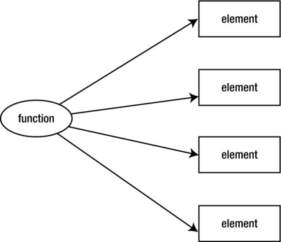
Figure 2-8. Apply a function to list elements
We do this in R with the apply() function.
The apply() function takes several parameters:
- First is our list.
- Next a number vector to indicate how we apply the function through the list (1 is for rows, 2 is for columns, and c[1,2] indicates both rows and columns).
- Finally is the function to apply to the list:
apply([list], [how to apply function], [function to apply])
Let’s look at an example. Let’s make a new matrix that we’ll call m. The matrix m will have ten columns and four rows:
> m <- matrix(c(1:40), byrow=FALSE, ncol=10)
> m
    [,1] [,2] [,3] [,4] [,5] [,6] [,7] [,8] [,9] [,10]
[1,]    1    5    9   13   17   21   25   29   33    37
[2,]    2    6   10   14   18   22   26   30   34    38
[3,]    3    7   11   15   19   23   27   31   35    39
[4,]    4    8   12   16   20   24   28   32   36    40
Now say we wanted to increment every number in the m matrix. We could simply use apply() as follows:
> apply(m, 2, function(x) x <- x + 1)
    [,1] [,2] [,3] [,4] [,5] [,6] [,7] [,8] [,9] [,10]
[1,]    2    6   10   14   18   22   26   30   34    38
[2,]    3    7   11   15   19   23   27   31   35    39
[3,]    4    8   12   16   20   24   28   32   36    40
[4,]    5    9   13   17   21   25   29   33   37    41
Do you see what we did there? We passed in m, we specified that we wanted to apply the function across the columns, and finally we passed in an anonymous function . The function accepts a parameter that we called x. The parameter x is a reference to the current matrix element. From there, we just increment the value of x by 1.
OK, say we wanted to do something slightly more interesting, such as zeroing out all the even numbers in the matrix. We could do the following:
> apply(m,c(1,2),function(x){if((x %% 2) == 0) x <- 0 else x <- x})
    [,1] [,2] [,3] [,4] [,5] [,6] [,7] [,8] [,9] [,10]
[1,]    1    5    9   13   17   21   25   29   33    37
[2,]    0    0    0    0    0    0    0    0    0     0
[3,]    3    7   11   15   19   23   27   31   35    39
[4,]    0    0    0    0    0    0    0    0    0     0
For the sake of clarity let’s break out that function that we are applying. We simply check to see whether the current element is even by checking to see whether it has a remainder when divided by two. If it is, we set it to zero; if it isn’t, we set it to itself:
function(x){
    if((x %% 2) == 0)
         x <- 0
    else
         x <- x
}
Functions
Speaking of functions, the syntax for creating functions in R is much like most other languages. We use the function keyword, give the function a name, have open and closed parentheses where we specify arguments, and wrap the body of the function in curly braces:
function [function name]([argument])
{
    [body of function]
}
Something interesting that R allows is the ... argument (sometimes called the dots argument). This allows us to pass in a variable number of parameters into a function. Within the function, we can convert the ... argument into a list and iterate over the list to retrieve the values within:
> offset <- function (...){
    for(i in list(...)){
         print(i)
    }
}
> offset(23,11)
[1] 23
[1] 11
We can even store values of different data types (modes) in the ... argument:
> offset("test value", 12, 100, "19ANM")
[1] "test value"
[1] 12
[1] 100
[1] "19ANM"
R uses lexical scoping. This means that when we call a function and try to reference variables that are not defined inside the local scope of the function, the R interpreter looks for those variables in the workspace or scope in which the function was created. If the R interpreter cannot find those variables in that scope, it looks in the parent of that scope.
If we create a function A within function B, the creation scope of function A is function B. For example, see the following code snippet:
> x <- 10
> wrapper <- function(y){
     x <- 99
     c<- function(y){
          print(x + y)
     }
     return(c)
}
> t <- wrapper()
> t(1)
[1] 100
> x
[1] 10
We created a variable x in the global space and gave it a value of 10. We created a function, named it wrapper, and had it accept an argument named y. Within the wrapper() function, we created another variable named x and gave it a value of 99. We also created a function named c. The function wrapper() passes the argument y into the function c(), and the c() function outputs the value of x added to y. Finally, the wrapper() function returns the c() function.
We created a variable t and set it to the returned value of the wrapper() function, which is the function c(). When we run the t() function and pass in a value of 1, we see that it outputs 100 because it is referencing the variable x from the function wrapper().
Being able to reach into the scope of a function that has executed is called a closure.
But, you may ask, how can we be sure that we are executing the returned function and not re-running wrapper() each time? R has a very nice feature where if you type in the name of a function without the parentheses, the interpreter will output the body of the function.
When we do this, we are in fact referencing the returned function and using a closure to reference the x variable:
> t
function(y){
         print(x + y)
    }
<environment: 0x17f1d4c4>
Summary
In this chapter, we downloaded and installed R. We explored the command line, went over data types, and got up and running importing into the R environment data for analysis. We looked at lists, how to create them, add to them, loop through them, and to apply functions to elements in a list.
We looked at functions, talked about lexical scope, and saw how to create closures in R.
Next chapter we’ll take a deeper dive into R, look at objects, get our feet wet with statistical analysis in R, and explore creating R markdown documents for distribution over the web.