![]()
Thus far when we have been talking about technologies used to create data visualizations we’ve been talking about R. We’ve spent the last two chapters exploring the R environment and learning about the command line. We covered introductory topics in the R language, ranging from data types, functions, and object-oriented programming. We even talked about how to publish our R documents to the Web using RPubs.
This chapter we will look at a JavaScript library called D3 that is used to create interactive data visualizations. First is a very quick primer on HTML, CSS, and JavaScript, the supporting languages of D3, to level set. Then we’ll dig into D3 and explore how to make some of the more commonly used charts in D3.
Preliminary Concepts
D3 is a JavaScript library. Specifically, that means it is written in JavaScript and embedded in an HTML page. We can reference the objects and functions in D3 in our own JavaScript code. So let’s start at the beginning. The purpose of the next section is not to take a deep dive into HTML CSS and JavaScript; there are plenty of other resources for that, including Foundation Website Creation that I helped to co-write. The purpose is to have a very high-level recap of concepts that we will deal with directly with D3. If you are already familiar with HTML, CSS, and JavaScript, you can skip down to the “History of D3” section of this chapter.
HTML
HTML is a markup language; in fact, it stands for HyperText Markup Language. It is a presentation language, made up of elements that signify formatting and layout. Elements contain attributes that have values that specify details about the element, tags, and content. To explain, let’s look at our basic HTML skeletal structure that we will use for most of our examples this chapter.
<!DOCTYPE html>
<html>
<head></head>
<body></body>
</html>
Let’s start at the first line. That is the doctype that tells the browser’s render engine what rule set to use. Browsers can support multiple versions of HTML, and each version has a slightly different rule set. The doctype are specified here is the HTML5 doctype. Another example of a doctype is this:
<!DOCTYPE html PUBLIC "-//W3C//DTD XHTML 1.1//EN""
 http://www.w3.org/TR/xhtml11/DTD/xhtml11.dtd ">
This is the doctype for XHTML 1.1. Notice that it specifies the URL of the document type definition (.dtd). If we were to read the plain text at the URL, we would see that it is a specification for how to parse HTML tags. The W3C maintains a list of doctypes here: http://www.w3.org/QA/2002/04/valid-dtd-list.html.
MODERN BROWSER ARCHITECTURE
Modern browsers are composed of modular pieces that encapsulate very specific functionality. These modules can also be licensed out and embedded in other applications:
- They have a UI layer that handles drawing the user interface of the browser, like the window, the status bar, and the back button.
- They render engines to parse, tokenize, and paint the HTML.
- They have a network layer to handle the network operations involved in retrieving the HTML and all the assets on the page.
- They have a JavaScript engine to interpret and execute the JavaScript in the page.
See Figure 4-1 for a representation of this architecture.
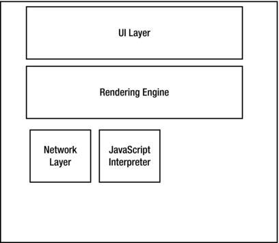
Figure 4-1. Modern Browser Architecture
Back to the skeletal HTML structure. The next line is the <html> tag, this is the root level tag for the document, and holds every other HTML element that we will use. Notice that there is a closing tag on the last line of the document.
Next is the <head> tag, which is a container that generally holds information that is not displayed on the page (for example, the title and meta information). After the <head> tag is the <body> tag, which is a container that holds all the HTML elements that will be displayed on the page; for example, paragraphs:
<p> this is a paragraph </p>
or links:
<a href="[URL]">link text or image here</a>
or images:
<img src="[URL]"/>
When it comes to D3, most of the JavaScript that we will be writing will be in the body section, and most of the CSS will be in the head section.
CSS
CSS stands for Cascading Style Sheets, and is what is used to style the HTML elements on a web page. Style sheets are either contained in <style> tags or linked to externally via <link> tags, and are comprised of style rules and selectors. Selectors target the element on the web page to style, and the style rule defines what styles to apply. Let’s look at an example:
<style>
p{
    color: #AAAAAA;
}
</style>
In the preceding code snippet, the style sheet is in a style tag. The p is the selector that tells the browser to target every paragraph tag on the web page. The style rule is wrapped in curly braces and is made up of properties and values. This case sets the color of the text in all the paragraphs to #AAAAAA which is the hexadecimal value of a light grey.
Selectors are where the real nuance of CSS is. This is relevant to us because D3 also uses CSS selectors to target elements. We can get very specific with selectors and target elements by class or id, or we can use pseudo-classes to target abstract concepts such as when an element is hovered over. We can target ancestors and descendants of elements, up and down the DOM.
![]() Note The DOM stands for the Document Object Model and is the application programming interface (API) that allows JavaScript to interact with the HTML elements that are on a web page.
Note The DOM stands for the Document Object Model and is the application programming interface (API) that allows JavaScript to interact with the HTML elements that are on a web page.
.classname{
/* style sheet for a class*/
}

#id{
/*stye sheet for an id*/
}

element:pseudo-class{

}
SVG
The next introductory concept for D3 is SVG, which stands for Scalable Vector Graphics. SVG, which is a standardized way to create vector graphics in the browser, is what D3 uses to create data visualizations. The core functionality that we are concerned about in SVG is the capability to draw shapes and text and integrate them into the DOM so that our shapes can be scripted via JavaScript.
![]() Note Vector graphics are graphics that are created using points and lines that are mathematically calculated and displayed by the rendering engine. Contrast this idea with bitmap or raster graphics in which the pixel display is prerendered.
Note Vector graphics are graphics that are created using points and lines that are mathematically calculated and displayed by the rendering engine. Contrast this idea with bitmap or raster graphics in which the pixel display is prerendered.
SVG is essentially its own markup language with its own doctype. We can write SVG in external .svg files or include the SVG tags directly in our HTML. Writing the SVG tags in our HTML page allows us to interact with our shapes via JavaScript.
SVG has support for predefined shapes as well as the capability to draw lines. The predefined shapes in SVG are these:
- <rect> to draw rectangles
- <circle> to draw circles
- <ellipse> to draw ellipses
- <line> to draw lines; also <polyline> and <polygon> to draw lines with multiple points
Let’s look at some code examples. If we will write our SVG into an HTML document, we use the <svg> tag to wrap our shapes. The <svg> takes the xmlns and version attributes. The xmlns attribute should be the path to the SVG namespace, and the version is obviously the version of SVG:
<svg xmlns=" http://www.w3.org/2000/svg " version="1.1">
</svg>
If we are writing standalone .svg files, we include the full doctype and xml tags to the page file:
<?xml version="1.0" standalone="no"?>
<!DOCTYPE svg PUBLIC "-//W3C//DTD SVG 1.1//EN" " http://www.w3.org/Graphics/SVG/1.1/DTD/svg11.dtd ">
<svg xmlns=" http://www.w3.org/2000/svg " version="1.1">
</svg>
Either way, we create our shapes within the <svg> tag. Let’s create some sample shapes in our <svg> tag:
<svg xmlns=" http://www.w3.org/2000/svg " version="1.1">
    <rect x="10" y="10" width="10" height="100" stroke="#000000" fill="#AAAAAA" />
    <circle cx="70" cy="50" r="40" stroke="#000000" fill="#AAAAAA" />
    <ellipse cx="230" cy="60" rx="100" ry="50" stroke="#000000" fill="#AAAAAA" />
</svg>
This code produces the shapes shown in Figure 4-2.
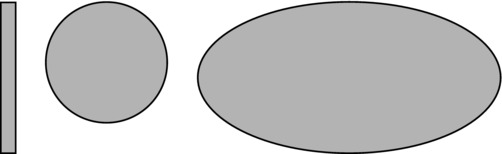
Figure 4-2. A rectangle, circle, and ellipse drawn in SVG
Notice that we assign x and y coordinates for all the shapes—in the case of the circle and ellipse cx and cy coordinates—as well as fill color and stroke colors. This is just the smallest taste; we can also create gradients and filters and then apply them to our shapes. We can also create text to use in our SVG drawings using the <text> tag.
Let’s take a look. We’ll update the preceding SVG code to add text labels for each shape:
<svg xmlns=" http://www.w3.org/2000/svg " version="1.1">
    <rect x="80" y="20" width="10" height="100" stroke="#000000" fill="#AAAAAA" />
    <text x="55" y="145" fill="#000000">rectangle</text>
    <circle cx="170" cy="60" r="40" stroke="#000000" fill="#AAAAAA" />
    <text x="150" y="145" fill="#000000">circle</text>
    <ellipse cx="330" cy="70" rx="100" ry="50" stroke="#000000" fill="#AAAAAA" />
    <text x="295" y="145" fill="#000000">ellipse</text>
</svg>
This code creates the drawing shown in Figure 4-3.
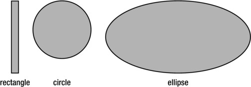
Figure 4-3. SVG shapes with text labels
Now we can start to see the possibilities of creating data visualizations with just these fundamental building blocks. Because D3 is a JavaScript library, and most of the work we will be doing with D3 will be in JavaScript, let’s next take a high-level look at JavaScript before we delve into D3.
JavaScript
JavaScript is the scripting language of the Web. JavaScript can be included in an HTML document either by placing script tags inline in the document or by linking to an external JavaScript document:
<script>
//javascript goes here
</script>

<script src="pathto.js"></script>
JavaScript can be used to process information, react to events, and interact with the DOM. In JavaScript, we create variables using the var keyword.
var foo = "bar";
Note that if we do not use the var keyword, the variable that we create is assigned to the global scope. We don’t want to do this because our globally scoped variable could then be overwritten by any other code on our web page.
JavaScript looks much like other C-based languages in that each expression ends in a semicolon, and blocks of code such as function and conditional bodies are wrapped in curly braces.
Conditional statements are generally if else statements formatted as follows:
if([condition]){
    [code to execute]
}else{
    [code to execute]
}
Functions are formatted like so:
function [function name] ([arguments]){
    [code to execute]
}
We access DOM elements in JavaScript usually by referencing the element by its id attribute. We do this like using the getElementById() function:
var header = document.getElementById("header");
The preceding code stores a reference to the element on the web page that has an ID of header. We can then update properties of this element, including adding new elements or removing the element altogether.
Objects in JavaScript are generally object literals, meaning that we craft them at runtime, composed of properties and methods. We create object literals like so:
var myObj = {
    myProp: 20,
    myfunc: function(){

    }
}
We reference properties and methods of objects using the dot operator:
myObj.myprop = 10;
See, that was fast and painless. Okay, on to D3!
History of D3
D3 stands for Data-Driven Documents and is a JavaScript library used to create interactive data visualizations. The seed of the idea that would become D3 started in 2009 as Protovis, created by Mike Bostock, Vadim Ogievetsky, and Jeff Heer while they were with the Stamford Visualization Group.
![]() Note Information on the Stamford Visualization group can be found at its website: http://vis.stanford.edu/. The original whitepaper for Protovis can be found at http://vis.stanford.edu/papers/protovis.
Note Information on the Stamford Visualization group can be found at its website: http://vis.stanford.edu/. The original whitepaper for Protovis can be found at http://vis.stanford.edu/papers/protovis.
Protovis was a JavaScript library that provided an interface for creating different types of visualizations. The root namespace was pv and it provided an API for creating bars and dots and areas, among other things. Like D3, Protovis used SVG to create these shapes; but unlike D3, it wrapped the SVG calls in its own proprietary nomenclature.
Protovis was abandoned in 2011, so its creators could take their learning and instead create and focus on D3. There is a difference in philosophy between Protovis and D3. Where Protovis aimed to provide wrapped functionality for creating data visualizations, D3 instead facilitates and streamlines the creation of data visualization by working with existing web standards and nomenclature. In D3, we create rectangles and circles in SVG, just facilitated by the syntactic sugar of D3.
Using D3
The first thing we need to do to get working with D3 is to go to the D3 website, http://d3js.org/, and download the latest version (see Figure 4-4).
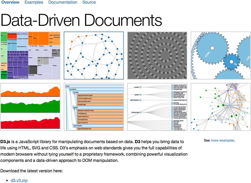
Figure 4-4. D3 homepage
After that is installed, you can set up a project.
Setting Up a Project
We can include the .js file directly on our page, like so:
<script src="d3.v3.js"></script>
The root namespace is d3; all the commands that we issue from D3 will be using the d3 object.
Using D3
We use the select() function to target specific elements or the selectAll() function to target all of a specific element type.
var body = d3.select("body");
The previous line selects the body tag and stores it in a variable named body. We can then change attributes of the body if we want to or add new elements to the body:
var allParagraphs = d3.select("body").selectAll("p");
The previous line selects the body tag and then selects all the paragraph tags within the body.
Notice that we chained the two actions together on the second line? We selected the body and then selected all the paragraphs, both actions chained together. Also note that we used the CSS selector to specify the element to target.
Okay, once we have selected an element that is now considered our selection and we can perform actions on that selection. We can select elements within our selection as we did in the previous example.
We can update attributes of the selection with the attr() function. The attr() function accepts two parameters: the first is the name of the attribute, and the second is the value to set the attribute to. Suppose we want to change the background color of the current document. We can just select the body and set the bgcolor attribute:
<script>
    d3.select("body")
         .attr("bgcolor", "#000000");
</script>
Notice in the previous code snippet that we have brought the chained attribute function call to the next line. We have done this for readability.
The really fun thing with this is that because we’re talking about JavaScript, and functions are first class objects in JavaScript, we can pass in a function as the value of an attribute so that whatever it evaluates to becomes the value that is set:
<script>
    d3.select("body")
         .attr("bgcolor", function(){
         return "#000000";
});
</script>
We can also add elements to our selection using the append() function. The append() function accepts a tag name as the first parameter. It will create a new element of the type specified and return that new element as the current selection:
<script>
var svg = d3.select("body")
         .append("svg");
</script>
The preceding code creates a new SVG tag in the body of the page and stores that selection in the variable svg.
Next let’s re-create the shapes in Figure 4-3 using what we’ve just learned about D3:
<script>
    var svg = d3.select("body")
         .append("svg")
         .attr("width", 800);

    var r = svg.append("rect")
         .attr("x", 80)
         .attr("y", 20)
         .attr("height", 100)
         .attr("width", 10)
         .attr("stroke", "#000000")
         .attr("fill", "#AAAAAA");

    var c = svg.append("circle")
         .attr("cx", 170)
         .attr("cy", 60)
         .attr("r", 40)
         .attr("stroke", "#000000")
         .attr("fill", "#AAAAAA");

    var e = svg.append("ellipse")
         .attr("cx", 330)
         .attr("cy", 70)
         .attr("rx", 100)
         .attr("ry", 50)
         .attr("stroke", "#000000")
         .attr("fill", "#AAAAAA");
</script>
For each shape we append a new element to the SVG element and update the attributes.
If we compare the two methods, we can see that we just create the SVG element in D3, just as we do in straight markup. We then create a SVG rectangle, circle, and ellipse inside the SVG element along with the same attributes that we specified in the SVG markup. But our D3 example has one very important difference: We now have references to each element on the page that we can interact with.
Let’s take a look at interactions in D3.
Binding Data
For data visualizations, the most important interaction we have with our SVG shapes is to bind data to them. This allows us to then reflect that data in the properties of the shapes.
To bind data, we simply call the data() method of a selection:
<script>
var rect = svg
    .append("rect")
    .data([1,2,3]);
</script>
That’s fairly straightforward. We can then reference that bound data via anonymous functions that we pass to our attr() function calls. Let’s take a look at an example.
First let’s create an array that we will call dataSet. To start to envision how this will correlate to creating a data visualization, you can think of dataSet as a list of nonsequential values, maybe test scores for a class or total rainfall for a set of regions:
<script>
var dataSet = [ 84,62,40,109];
</script>
Next we will create an SVG element on the page. To do that, we’ll select the body and append an SVG element with a width of 800 pixels. We’ll keep a reference to this SVG element in a variable called svg:
<script>
var svg = d3
    .select("body")
    .append("svg")
    .attr("width", 800);
</script>
Here is where being able to bind data changes things. We will chain together a series of commands that will create placeholder rectangles in the SVG element based on how many elements exist in our data array.
We will first use selectAll() to return a reference to all rectangles in the SVG element. There are none yet, but there will be by the time the chain finishes executing. Next in the chain, we bind our dataSet variable and call enter(). The enter() function creates placeholder objects from the bound data. Finally, we call append() to create a rectangle at each placeholder that enter() created:
<script>
bars = svg
    .selectAll("rect")
    .data(dataSet)
    .enter()
    .append("rect");
</script>
If we looked at our work so far in a browser we would see a blank page, but if we looked at the HTML in a web inspector such as Firebug, we would see the SVG element along with the rectangles created, but with no styling or attributes specified yet, similar to Figure 4-5.
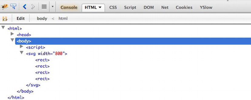
Figure 4-5. Caption
Next, let’s style the rectangles that we just made. We have a reference to all the rectangles in the variable bars, so let’s chain together a bunch of attr() calls to style the rectangles. While we’re at it, let’s use our bound data to size the height of the bars:
<script>

bars
    .attr("width", 15 )
    .attr("height", function(x){return x;})
    .attr("x", function(x){return x + 40;})
    .attr("fill", "#AAAAAA")
    .attr("stroke", "#000000");

</script>
The full source code looks like the following and makes the shapes that we see in Figure 4-6:
<script>
var dataSet = [84,62,40,109];

var svg = d3
    .select("body")
    .append("svg")
    .attr("width", 800);

bars = svg
    .selectAll("rect")
    .data(dataSet)
    .enter()
    .append("rect");

bars
    .attr("width", 15 )
    .attr("height", function(x){return x;})
    .attr("x", function(x){return x + 40;})
    .attr("fill", "#AAAAAA")
    .attr("stroke", "#000000");

</script>
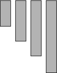
Figure 4-6. Styled rectangles for bar chart
Now look in Firebug again; you can see the generated markup, as shown in Figure 4-7.
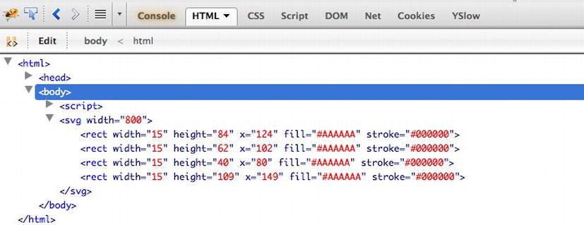
Figure 4-7. Rectangles shown as SVG source code in Firebug
Now you can really see the beginnings of how we can start to make data visualizations with D3 by binding data to SVG shapes. Let’s take this concept another step forward.
Creating a Bar Chart
Our example so far looks a lot like the start of a bar chart in that we have a number of bars whose heights represent data. Let’s give it some structure.
First, let’s give our SVG container a more concrete width and height. This is important because the size of the SVG container is what determines the scale we use to normalize the rest of the chart. And because we will reference this sizing throughout our code, let’s make sure we abstract these values into their own variables.
We will define a height and width for our SVG container. We’ll also create variables that will hold the minimum and maximum values that we will use on our axes: 0 and 109, respectively. We’ll also define an offset value so we can draw the SVG container slightly larger than our chart to give the chart margins around it:
<script>
var chartHeight = 460,
    chartWidth = 400,
    chartMin = 0,
    chartMax = 109,
    offset = 60

var svg = d3
    .select("body")
    .append("svg")
    .attr("width", chartWidth)
    .attr("height", chartHeight + offset);
</script>
We next need to fix the orientation of our bars. As shown in Figure 4-6, the bars are drawn from the top down, so that although their heights are accurate, they appear to be facing down because SVG draws and positions shapes from the top left. So to get them correctly oriented so the bars look like they are coming up from the bottom of the chart, let’s add a y attribute to our bars.
The y attribute should be a function that references the data; this function should subtract the bar height value from the chart height. The returned value from this function is the value used in the y coordinate:
<script>
bars
    .attr("width", 15 )
    .attr("height", function(x){return x;})
    .attr("y", function(x){return (chartHeight - x);})
    .attr("x", function(x){return x;})
    .attr("fill", "#AAAAAA")
    .attr("stroke", "#000000");
</script>
This flips the bars to the bottom of the SVG element. We can see the results in Figure 4-8.
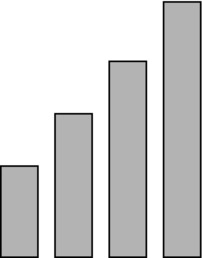
Figure 4-8. Rectangles in bar chart no longer inverted
Now let’s scale the bars to fit the height of the SVG element. To do this, we’ll use a D3 scale() function. The scale() function is used to take a number within a range and transform it to the equivalent of that number in a different range of numbers, essentially to scale values to equivalent values.
In this case, we have a number range that signifies the range of values in our dataSet array, which signify the heights of the bars, and we want to transform these numbers to equivalent values:
<script>
var yscale = d3.scale.linear()
    .domain([chartMin,chartMax])
    .range([0,(chartHeight)]);
</script>
We then just update the height and y attributes of the bars to use the yscale() function:
<script>
bars
    .attr("width", 15 )
    .attr("height", function(x){ return yscale(x);})
    .attr("y", function(x){return (chartHeight - yscale(x));})
    .attr("x", function(x){return x;})
    .attr("fill", "#AAAAAA")
    .attr("stroke", "#000000");
</script>
This produces the graphic shown in Figure 4-9.
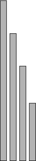
Figure 4-9. Rectangles for bar chart properly scaled
Very nice! But so far, we’ve just been placing the bars based on their height instead of where they lie in the array. Let’s change that to make their array location more meaningful, so the bars are displayed in the correct order.
To do that, we just update the x value of the bars. We’ve seen already that we can pass in an anonymous function to the value parameter of the attr() function. The first parameter in our anonymous function is the value of the current element of our array. If we specify a second parameter in our anonymous function, it will hold the current index number.
We can then reference that value and offset it to place each bar:
<script>
bars
    .attr("width", 15 )
    .attr("height", function(x){ return yscale(x);})
    .attr("y", function(x){return (chartHeight - yscale(x));})
    .attr("x", function(x, i){return (i * 20);})
    .attr("fill", "#AAAAAA")
    .attr("stroke", "#000000");
</script>
This gives us the ordering of the bars shown in Figure 4-10. Just by eyeballing it, we can tell that the bars are now closer representations of the data in the array—not just the height but also the height in the order specified in the array.
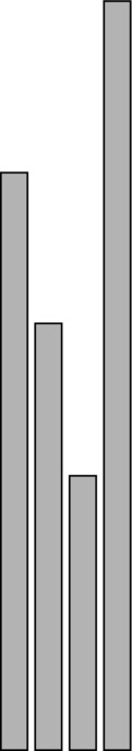
Figure 4-10. Rectangles in bar chart ordered to follow the ordering in our data
Now let’s add text labels so that we can better see what values the heights of the bars are signifying.
We do that by creating SVG text elements in much the same way as creating the bars. We create text placeholders for every element in our data array and then style the text elements. You’ll notice that the anonymous function that we pass into the x and y attribute calls is almost the same for the text elements as it was for the bars, only offset so that the text is above and to the center of each bar:
<script>
svg.selectAll("text")
    .data(dataSet)
    .enter()
    .append("text")
    .attr("x", function(d) { return (d * 20); })
    .attr("y", function(x){return (chartHeight - yscale(x)) ;})
    .attr("dx", -15/2)
    .attr("dy", "1.2em")
    .attr("text-anchor", "middle")
    .text(function(d) { return d;})
    .attr("fill", "black");

</script>
This code produces the chart shown in Figure 4-11.
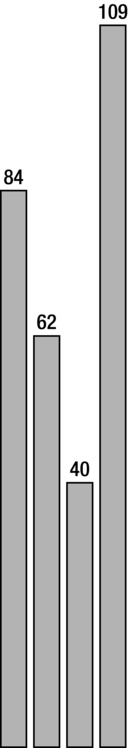
Figure 4-11. Bar chart with text labels
See the following complete source code:
<html>
<head>
<title></title>
<script src="d3.v3.js"></script>
</head>
<body>
<script>
var dataSet = [84,62,40,109];

var chartHeight = 460,
    chartWidth = 400,
    chartMin = 0,
    chartMax = 115,
    offset = 60;

var yscale = d3.scale.linear()
    .domain([chartMin,chartMax])
    .range([0,(chartHeight)]);

var svg = d3
    .select("body")
    .append("svg")
    .attr("width", chartWidth)
    .attr("height", chartHeight + offset);


bars = svg
    .selectAll("rect")
    .data(dataSet)
    .enter()
    .append("rect");

bars
    .attr("width", 15 )
    .attr("height", function(x){ return yscale(x);})
    .attr("y", function(x){return (chartHeight - yscale(x));})
    .attr("x", function(x, i){return (i * 20);})
    .attr("fill", "#AAAAAA")
    .attr("stroke", "#000000");

svg.selectAll("text")
    .data(dataSet)
    .enter()
    .append("text")
    .attr("x", function(d) { return (d * 20); })
    .attr("y", function(x){return (chartHeight - yscale(x)) ;})
    .attr("dx", -15/2)
    .attr("dy", "1.2em")
    .attr("text-anchor", "middle")
    .text(function(d) { return d;})
    .attr("fill", "black");

</script>
</body>
</html>
And finally let’s read in our data from external files instead of hard-coding it in the page.
Loading External Data
First, we’ll take the array out of our file and put it in its own external file: sampleData.csv. The contents of sampleData.csv are simply the following:
84,62,40,109
Next we will use the d3.text() function to load in sampleData.csv. The way d3.text() works is that it takes a path to an external file as the first parameter, and as the second parameter it takes a function. The function receives a parameter that is the contents of the external file:
<script>
d3.text("sampleData.csv", function(data) {});
</script>
The catch is that we need the contents of our external file before we can begin doing any charting on the data. So within the callback function, we will parse up the file and then wrap all our existing functionality, like so:
<html>
<head>
<title></title>
<script src="d3.v3.js"></script>
</head>
<body>
<script>

d3.text("sampleData.csv", function(data) {
var dataSet = data.split(",");

var chartHeight = 460,
    chartWidth = 400,
    chartMin = 0,
    chartMax = 115,
    offset = 60;

var yscale = d3.scale.linear()
    .domain([chartMin,chartMax])
    .range([0,(chartHeight)]);

var svg = d3
    .select("body")
    .append("svg")
    .attr("width", chartWidth)
    .attr("height", chartHeight + offset);


bars = svg
    .selectAll("rect")
    .data(dataSet)
    .enter()
    .append("rect");

bars
    .attr("width", 15 )
    .attr("height", function(x){ return yscale(x);})
    .attr("y", function(x){return (chartHeight - yscale(x));})
    .attr("x", function(x, i){return (i * 20);})
    .attr("fill", "#AAAAAA")
    .attr("stroke", "#000000");

svg.selectAll("text")
    .data(dataSet)
    .enter()
    .append("svg:text")
    .attr("x", function(d, i) { return (i * 20) })
    .attr("y", function(x){return (chartHeight - yscale(x));})
    .attr("dx", -15/2)
    .attr("dy", "1.2em")
    .attr("text-anchor", "middle")
    .text(function(d) { return d;})
    .attr("fill", "black");

})

</script>
</body>
</html>
And CSV files aren’t the only format we can read in. In fact, d3.text() is only syntactic sugar—a convenience method or a type-specific wrapper for D3’s implementation of the XMLHttpRequest object d3.xhr().
For reference, the XMLHttpRequest object is what is used in AJAX transactions to load content asynchronously from the client side without refreshing the page. In pure JavaScript, we instantiate the XHR object, pass in an URL to a resource, and the method to retrieve the resource (GET or POST). We also specify a callback function that will get invoked when the XHR object is updated. In this function, we can parse up the data and begin using it. See Figure 4-12 for a high-level diagram of this process.
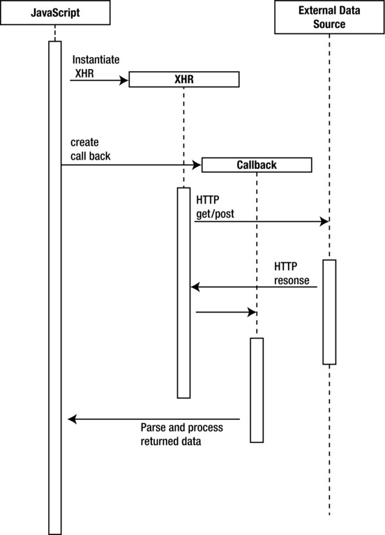
Figure 4-12. Sequence diagram of XHR transaction
In D3 is the d3.xhr() function that is D3’s wrapper for the XMLHttpRequest object. It works much the same way that we just saw d3.text() work, where we pass in a URL to a resource and a callback function to execute.
The other type-specific convenience functions that D3 has are d3.csv(), d3.json(), d3.xml(), and d3.html().
Summary
This chapter explored D3. We started out covering the introductory concepts of HTML, CSS, SVG and JavaScript, at least the points that are pertinent to implementing D3. From there we delved into D3, looking at introductory concepts like creating our first SVG shapes to expanding on that idea by making those shapes into a bar graph.
D3 is a fantastic library for crafting data visualizations. To see the full API documentation, see https://github.com/mbostock/d3/wiki/API-Reference.
We will return to D3, but first we will explore some data visualizations that we can create that have practical application in the world of web development. The first one we will look at is something that you may have seen in your Google analytics dashboard or something similar: a data map based on user visits.