
![]()
Visualizing Spatial Data from Access Logs
In the last chapter, we talked about D3 and looked at concepts from making simple shapes to creating a bar chart out those shapes. In the previous two chapters, we took a deep dive into R. Now that you are familiar with the core technologies that we will be using, let’s begin looking at examples of how, as web developers, we can create data visualizations that communicate useful information around our domain.
The first one that we will look at is creating a data map out of our access logs.
First, let’s level set and make sure that we clearly define a data map. A data map is a representation of information over a spatial field, a marriage of statistics with cartography. Data maps are some of the most easily understood and widely used data visualizations there are because their data is couched in something that we are all familiar with and use anyway: maps.
Recall the discussion in Chapter 1 of the Cholera map created by Jon Snow in 1854. This is considered one of the earliest examples of a data map, though there are several notable contemporaries, including several by Charles Minard, an engineer in nineteenth-century France. He is most widely remembered for his data visualization of Napoleon’s invasion of Russia in 1812.
Minard also created several prominent data maps. Two of his most famous data maps include the data map demonstrating the source region and percentage of total cattle consumed in France (see Figure 5-1), and the data map demonstrating the wine export path and destination from France (see Figure 5-2).
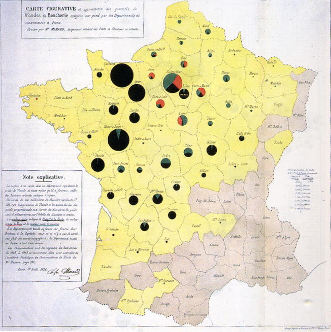
Figure 5-1. Early data map from Charles Minard demonstrating source region and cattle consumption in France
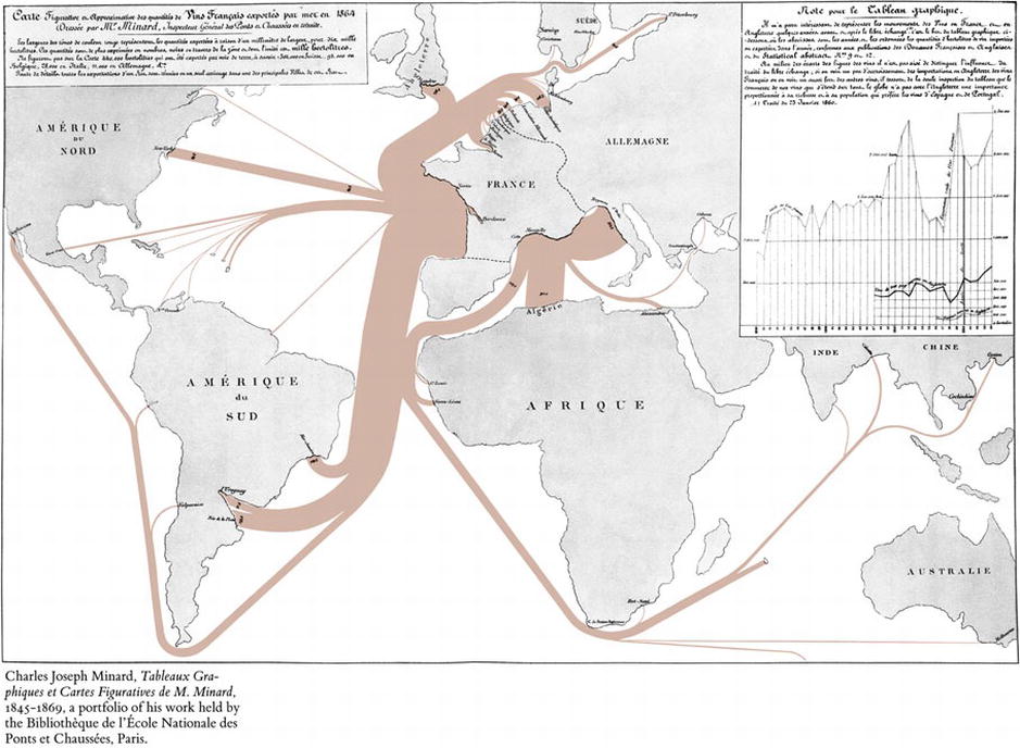
Figure 5-2. Data map from Minard demonstrating wine export path and destination
Today we see data maps everywhere. They can be informative and artistic expressions, like the wind map project from Fernanda Viegas and Martin Wattenberg (see Figure 5-3). Available at http://hint.fm/wind, the wind project demonstrates the path and force of wind currents over the United States.
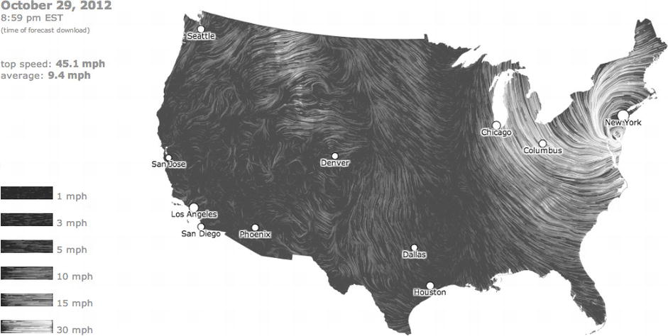
Figure 5-3. Wind map, showing wind speeds by region for the touchdown of Hurricane Sandy (used with permission of Fernanda Viegas and Martin Wattenberg)
Data maps can be profound, such as those available at energy.gov that demonstrate concepts such as energy consumption by state (see Figure 5-4), or even renewable energy production by state.
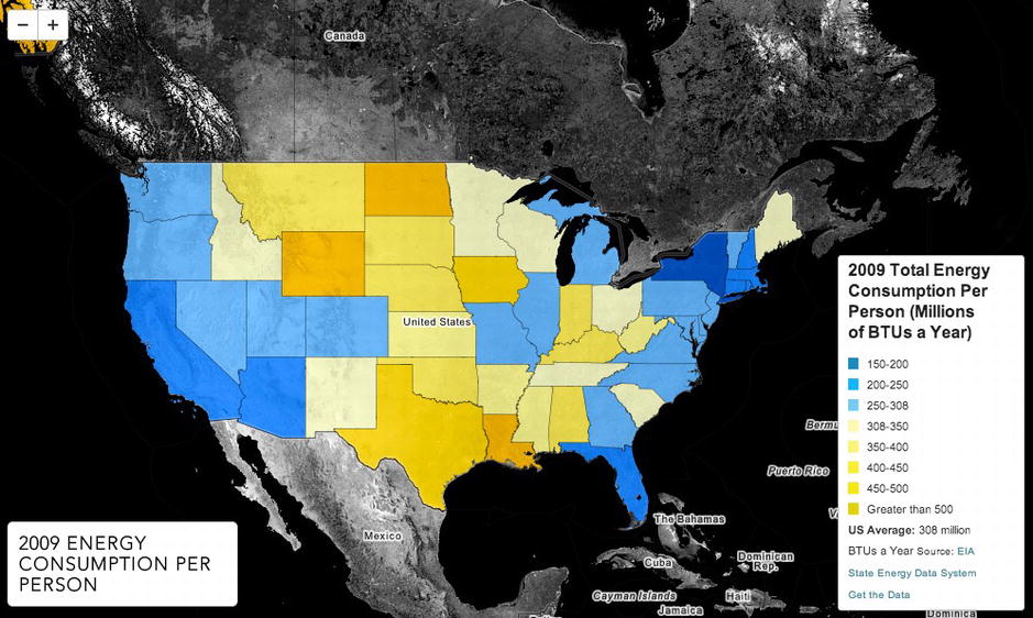
Figure 5-4. Data map depicting energy consumption by state, from energy.gov, (available at http://energy.gov/maps/2009-energy-consumption-person)
You’ve now seen historical and contemporary examples of data maps. In this chapter, you will look at creating your own data map from web server access logs.
Access Logs
Access logs are records that a web server keeps to track what resources were requested. Whenever a web page, an image, or any other kind of file is requested from a server, the server makes a log entry for the request. Each request has certain data points associated with it, usually information about the requestor of the resource (for example, IP address and user agent) and general information such as time of day and what resource was requested.
Let’s look at an access log. A sample entry looks like this:
msnbot-157-55-17-199.search.msn.com - - [18/Jan/2013:13:32:15 -0400] "GET /robots.txt HTTP/1.1" 404 208 "-" "Mozilla/5.0 (compatible; bingbot/2.0; + http://www.bing.com/bingbot.htm )"
This is a snippet from a sample Apache access log. Apache access logs follow the combined log format, which is an extension of the common log format standard of the World Wide Web Consortium (W3C). Documentation for the common log format can be found here:
http://www.w3.org/Daemon/User/Config/Logging.html#common-logfile-format
The common log format defines the following fields, separated by tabs:
- IP address or DNS name of remote host
- Logname of the remote user
- Username of the remote user
- Datestamp
- The request; usually includes the request method and the path to the resource requested
- HTTP status code returned for the request
- Total file size of the resource requested
The combined log format adds the referrer and user agent fields. The Apache documentation for the combined log format can be found here:
http://httpd.apache.org/docs/current/logs.html#combined
Note that fields that are not available are represented by a single dash -.
Let’s dissect the previous log entry.
- The first field is msnbot-157-55-17-199.search.msn.com. This is a DNS name that just happens to have the IP address built into it. We can’t count on parsing the IP address out of this domain, so for now just ignore the IP address. When we get to programmatically parsing the logs we will use the native PHP function gethostbyname() to look up the IP addresses for given domain names.
- The next two fields, the logname and the user, are empty.
- Next is the datestamp: [18/Jan/2013:13:32:15 -0400].
- After the datestamp is the request: "GET /robots.txt HTTP/1.1". If you hadn’t already guessed from the DNS name, this is a bot, specifically Microsoft’s msnbot replacement: the bingbot. In this record, the bingbot is requesting the robots.txt file.
- Next is the HTTP status of the request: 404. Clearly there was no robots.txt file available.
- Next is the total payload of the request. Apparently the 404 cost 208 bytes.
- Next is a dash to signify that the referrer was empty.
- Finally is the useragent: "Mozilla/5.0 (compatible; bingbot/2.0; + http://www.bing.com/bingbot.htm )", which tells us definitively that it is indeed a bot.
Now that you have the access log and understand what is in it, you can parse it to use each field in it programmatically.
Parsing the Access Log
The process of parsing the access log is the following:
- Read in the access log.
- Parse it and gather geographic data based on the stored IP address.
- Output the fields that we are interested in for our visualization.
- Read in this output and visualize.
We’ll use PHP for the first three steps and R for the last step. Note that you will need to be running PHP 5.4.10 or higher to successfully run the following PHP code.
Read in the Access Log
Create a new PHP document called parseLogs.php, within which you will first create a function to read in a file. Call this function parseLog() and have it accept the path to the file:
function parseLog($file){

}
Within this function, you will write some code that will open the passed in file for reading and iterate through each line of the file until it reaches the end of the file. Each step in the iteration stores the line that is read in, in the variable $line:
$logArray = array();
$file_handle = fopen($file, "r");
while (!feof($file_handle)) {
     $line = fgets($file_handle);
}
fclose($file_handle);
Fairly standard file I/O functionality in PHP so far. Within the loop, you will stub out a function call to a function that you will call parseLogLine() and another function that you will call getLocationbyIP(). In parseLogLine(), you will split up the line and store the values in an array. In getLocationbyIP(), you will use the IP address to get geographic information. You will then store this returned array in a larger array that called $logArray.
$lineArr = parseLogLine($line);
$lineArr = getLocationbyIP($lineArr);
$logArray[count($logArray)] = $lineArr;
Don’t forget to create the $logArray variable at the top of the function.
The finished function should look like so:
function parseLog($file){
$logArray = array();
$file_handle = fopen($file, "r");
while (!feof($file_handle)) {
     $line = fgets($file_handle);
     $lineArr = parseLogLine($line);
     $lineArr = getLocationbyIP($lineArr);
     $logArray[count($logArray)] = $lineArr;
}
fclose($file_handle);
return $logArray;
}
Parse the Log File
Next you’ll flesh out the parseLogLine() function. First you’ll create the empty function:
function parseLogLine($logLine){
}
The function will expect a single line of the access log.
Remember that each line of the access log is made up of sections of information separated by whitespace. Your first instinct might be to just split the line at each instance of a whitespace, but this would result in breaking up the user agent string (and potentially other fields) in unexpected ways.
For our purposes, a much cleaner way to parse the line is to use a regular expression. Regular expressions, called regex for short, are patterns that enable you to do quick and efficient string matching.
Regular expressions use special characters to define these patterns: individual characters, character literals, or sets of characters. A deep dive on regular expressions is outside of the scope of this chapter, but a great reference to read about the different regular expression patterns is the Microsoft regular expression Quick Reference, available here: http://msdn.microsoft.com/en-us/library/az24scfc.aspx.
Grant Skinner also provides a great tool for creating and debugging regular expressions (see Figure 5-5), which is available here: http://gskinner.com/RegExr/.
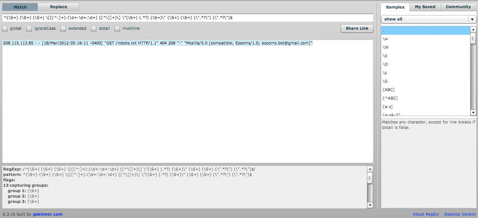
Figure 5-5. Grant Skinner’s regex tool
Let’s define our regular expression pattern and store it in a variable that we will call $pattern.
If you aren’t proficient with regex, you can create them fairly easily using Grant Skinner’s tool (refer to Figure 5-5). Using this tool, you can come up with the following pattern:
$pattern = "/^(S+) (S+) (S+) [([^:]+):(d+:d+:d+) ([^]]+)] "(S+) (.*?) (S+)" (S+) (S+) (".*?") (".*?")$/";
Within the tool, you can see how it breaks up the strings into the following groups (see Figure 5-6).
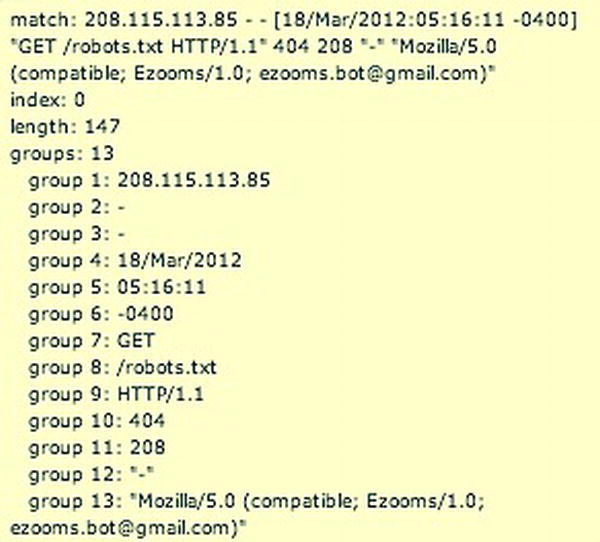
Figure 5-6. Log file line split into groups
You now have a regular expression to use. Let’s use PHP’s preg_match() function. This takes as parameters a regular expression, a string to match it against, and an array to populate as the output of the pattern matching:
preg_match($pattern,$logLine,$logs);
From there, we can just create an associative array with named indexes to hold our parsed up line:
$logArray = array();
$logArray['ip'] = gethostbyname($logs[1]);
$logArray['identity'] = $logs[2];
$logArray['user'] = $logs[2];
$logArray['date'] = $logs[4];
$logArray['time'] = $logs[5];
$logArray['timezone'] = $logs[6];
$logArray['method'] = $logs[7];
$logArray['path'] = $logs[8];
$logArray['protocol'] = $logs[9];
$logArray['status'] = $logs[10];
$logArray['bytes'] = $logs[11];
$logArray['referer'] = $logs[12];
$logArray['useragent'] = $logs[13];
Our complete parseLogLine() function should now look like this:
function parseLogLine($logLine){
        $pattern = "/^(S+) (S+) (S+) [([^:]+):(d+:d+:d+) ([^]]+)] "(S+) (.*?) (S+)" (S+) (S+) (".*?") (".*?")$/";

        preg_match($pattern,$logLine,$logs);

        $logArray = array();
        $logArray['ip'] = gethostbyname($logs[1]);
        $logArray['identity'] = $logs[2];
        $logArray['user'] = $logs[2];
        $logArray['date'] = $logs[4];
        $logArray['time'] = $logs[5];
        $logArray['timezone'] = $logs[6];
        $logArray['method'] = $logs[7];
        $logArray['path'] = $logs[8];
        $logArray['protocol'] = $logs[9];
        $logArray['status'] = $logs[10];
        $logArray['bytes'] = $logs[11];
        $logArray['referer'] = $logs[12];
        $logArray['useragent'] = $logs[13];

        return $logArray;

}
Next you will create the functionality for the getLocationbyIP() function.
Geolocation by IP
In the getLocationbyIP() function, you can take the array that you made by parsing a line of the access log and use the IP field to get the geographic location. There are many ways to get geographic location by IP address; most involve either calling a third-party API or downloading a third-party database with the IP location information prepopulated. Some of these third parties are freely available; some have a cost associated with them.
For our purposes, you can use the free API available at hostip.info. Figure 5-7 shows the hostip.info home page.
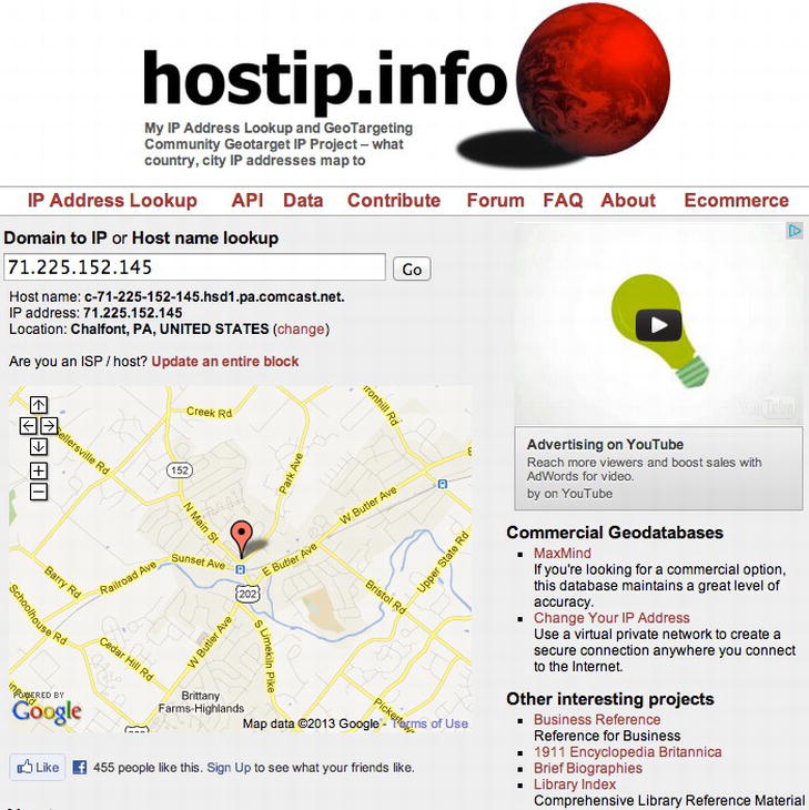
Figure 5-7. hostip.info home page
The hostip.info service aggregates geotargeting information from ISPs as well as direct feedback from users. It exposes an API as well as a database available for download.
The API is available at http://api.hostip.info/. If no parameters are provided, the API returns the geo location of the client. By default, the API returns XML. The return value looks like this:
<?xml version="1.0" encoding="ISO-8859-1" ?>
<HostipLookupResultSet version="1.0.1" xmlns:gml=" http://www.opengis.net/gml " xmlns:xsi=" http://www.w3.org/2001/XMLSchema-instance " xsi:noNamespaceSchemaLocation=" http://www.hostip.info/api/hostip-1.0.1.xsd ">
 <gml:description>This is the Hostip Lookup Service</gml:description>
 <gml:name>hostip</gml:name>
 <gml:boundedBy>
  <gml:Null>inapplicable</gml:Null>
 </gml:boundedBy>
 <gml:featureMember>
  <Hostip>
   <ip>71.225.152.145</ip>
   <gml:name>Chalfont, PA</gml:name>
   <countryName>UNITED STATES</countryName>
   <countryAbbrev>US</countryAbbrev>
   <!-- Co-ordinates are available as lng,lat -->
   <ipLocation>
    <gml:pointProperty>
     <gml:Point srsName=" http://www.opengis.net/gml/srs/epsg.xml#4326 ">
      <gml:coordinates>-75.2097,40.2889</gml:coordinates>
     </gml:Point>
    </gml:pointProperty>
   </ipLocation>
  </Hostip>
 </gml:featureMember>
</HostipLookupResultSet>
You can refine the API calls. If you want only country information, you can call http://api.hostip.info/country.php. It returns a string with a country code. If JSON is preferred over XML, you can call http://api.hostip.info/get_json.php and get the following result:
{"country_name":"UNITED STATES","country_code":"US","city":"Chalfont, PA","ip":"71.225.152.145"}
To specify an IP address, add the parameter ?ip=xxxx, like so:
http://api.hostip.info/get_json.php?ip=100.43.83.146
OK, let’s code the function!
We’ll stub out the function and have it accept an array. We’ll pull the IP address from the array, store it in a variable, and concatenate the variable to a string that contains the path to the hostip.info API:
function getLocationbyIP($arr){
     $IPAddress = $arr['ip'];
     $IPCheckURL = " http://api.hostip.info/get_json.php?ip=$IPAddress ";
}
You’ll pass this string to the native PHP function file get_contents() and store the return value, the results of the API call, in a variable that you’ll name jsonResponse. You’ll use the PHP json_decode() function to convert the returned JSON data into a native PHP object:
$jsonResponse =  file_get_contents($IPCheckURL);
$geoInfo = json_decode($jsonResponse);
You next pull the geolocation data from the object and add it to the array that you passed into the function. The city and state information is a single string separated by a comma and a space (“Philadelphia, PA”), so you’ll need to split at the comma and save each field separately in the array.
$arr['country'] = $geoInfo->{"country_code"};
$arr['city'] = explode(",",$geoInfo->{"city"})[0];
$arr['state'] = explode(",",$geoInfo->{"city"})[1];
Next let’s do a little bit of error checking that will make things easier later on in the process. You’ll check to see whether the state string has any value; if it doesn’t, set it to “XX”. This will be helpful once you begin parsing data in R. And finally you’ll return the updated array:
if(count($arr['state']) < 1)
     $arr['state'] = "XX";
return $arr;
The full function should look like this:
function getLocationbyIP($arr){
     $IPAddress = $arr['ip'];
     $IPCheckURL = " http://api.hostip.info/get_json.php?ip=$IPAddress ";

     $jsonResponse =  file_get_contents($IPCheckURL);
     $geoInfo = json_decode($jsonResponse);
     $arr['country'] = $geoInfo->{"country_code"};
     $arr['city'] = explode(",",$geoInfo->{"city"})[0];
     $arr['state'] = explode(",",$geoInfo->{"city"})[1];
     if(count($arr['state']) < 1)
          $arr['state'] = "XX";
     return $arr;
}
Finally, let’s create a function to write processed data out to a file.
Output the Fields
You’ll create a function named writeRLog() that accepts two parameters: the array populated with decorated log data and the path to a file:
function writeRLog($arr, $file){
}
You need to create a variable called writeFlag that will be the flag to tell PHP to either write or append data to the file. You check to see whether the file exists; if it does, you append content instead of overwrite. After the check, open the file:
writeFlag = "w";
if(file_exists($file)){
     $writeFlag = "a";
}
$fh = fopen($file, $writeFlag) or die("can't open file");
You then loop through the passed-in array; construct a string containing the IP address, date, HTTP status, country code, state, and city of each log entry; and write that string to the file. Once you’ve finished iterating through the array, you close the file:
for($x = 0; $x < count($arr); $x++){
     if($arr[$x]['country'] != "XX"){
          $data = $arr[$x]['ip'] . "," . $arr[$x]['date'] . "," . $arr[$x]['status'] . "," . $arr[$x]['country'] . "," . $arr[$x]['state'] . "," . $arr[$x]['city'];
      }
      fwrite($fh, $data . "
");
 }
Our completed writeRLog() function should look like this:
function writeRLog($arr, $file){
     $writeFlag = "w";
     if(file_exists($file)){
          $writeFlag = "a";
          }
          $fh = fopen($file, $writeFlag) or die("can't open file");
          for($x = 0; $x < count($arr); $x++){
               if($arr[$x]['country'] != "XX"){
                    $data = $arr[$x]['ip'] . "," . $arr[$x]['date'] . "," . $arr[$x]['status'] . "," . $arr[$x]['country'] . "," . $arr[$x]['state'] . "," . $arr[$x]['city'];
               }
               fwrite($fh, $data . "
");
          }
     fclose($fh);
     echo "log created";
}
Adding Control Logic
Finally you’ll create some control logic to invoke all these functions that you just created. You’ll declare the path to the access log and the path to our output flat file, call parseLog() and send the output to writeRLog():
$logfile = "access_log";
$chartingData = "accessLogData.txt";
$logArr = parseLog($logfile);
writeRLog($logArr, $chartingData);
Our completed PHP code should look like the following:
<html>
<head></head>
<body>
<?php
$logfile = "access_log";
$chartingData = "accessLogData.txt";
$logArr = parseLog($logfile);
writeRLog($logArr, $chartingData);

function parseLog($file){
        $logArray = array();
        $file_handle = fopen($file, "r");
        while (!feof($file_handle)) {
           $line = fgets($file_handle);
           $lineArr = parseLogLine($line);
           $lineArr = getLocationbyIP($lineArr);
           $logArray[count($logArray)] = $lineArr;
        }
        fclose($file_handle);
        return $logArray;
}

function parseLogLine($logLine){
        $pattern = "/^(S+) (S+) (S+) [([^:]+):(d+:d+:d+) ([^]]+)] "(S+) (.*?) (S+)" (S+) (S+) (".*?") (".*?")$/";


        preg_match($pattern,$logLine,$logs);

        $logArray = array();
        $logArray['ip'] = gethostbyname($logs[1]);
        $logArray['identity'] = $logs[2];
        $logArray['user'] = $logs[2];
        $logArray['date'] = $logs[4];
        $logArray['time'] = $logs[5];
        $logArray['timezone'] = $logs[6];
        $logArray['method'] = $logs[7];
        $logArray['path'] = $logs[8];
        $logArray['protocol'] = $logs[9];
        $logArray['status'] = $logs[10];
        $logArray['bytes'] = $logs[11];
        $logArray['referer'] = $logs[12];
        $logArray['useragent'] = $logs[13];

        return $logArray;

}

function getLocationbyIP($arr){
        $IPAddress = $arr['ip'];
        $IPCheckURL = " http://api.hostip.info/get_json.php?ip=$IPAddress ";

        $jsonResponse =  file_get_contents($IPCheckURL);
        $geoInfo = json_decode($jsonResponse);
        $arr['country'] = $geoInfo->{"country_code"};
        $arr['city'] = explode(",",$geoInfo->{"city"})[0];
        $arr['state'] = explode(",",$geoInfo->{"city"})[1];

        return $arr;
}

function writeRLog($arr, $file){
        $writeFlag = "w";
        if(file_exists($file)){
                $writeFlag = "a";
        }
        $fh = fopen($file, $writeFlag) or die("can't open file");
        for($x = 0; $x < count($arr); $x++){
                if($arr[$x]['country'] != "XX"){
                        $data = $arr[$x]['ip'] . "," . $arr[$x]['date'] . "," . $arr[$x]['status'] . "," . $arr[$x]['country'] . "," . $arr[$x]['state'] . "," . $arr[$x]['city'];
                }
                fwrite($fh, $data . "
");
        }
        fclose($fh);
        echo "log created";
}
?>
</body>
</html>
And it should produce a flat file that looks like so:
157.55.32.94,25/Jan/2013,404,US, WA,Redmond
180.76.6.26,25/Jan/2013,200,CN,,Beijing
213.174.154.106,25/Jan/2013,301,UA,,(Unknown city)
We have made a sample access log available here: http://tom-barker.com/data/access_log.
So far, you parsed the access log, scrubbed the data, decorated it with location information, and created a flat file that has a subset of information. The next step is to visualize this data.
Because you are making a map, you need to install the map package. Open up R; from the console, type the following:
> install.packages('maps')
> install.packages('mapproj')
Now we can begin! To reference the map package in the R script, you need to load it into memory by calling the library() function:
library(maps)
library(mapproj)
You next create several variables—one to point to our formatted access log data; another is a list of column names. You create a third variable, logData, to hold the data frame created when you read in the flat file:
logDataFile <- '/Applications/MAMP/htdocs/accessLogData.txt'
logColumns <- c("IP", "date", "HTTPstatus", "country", "state", "city")
logData <- read.table(logDataFile, sep=",", col.names=logColumns)
If you type logData in the console, you see the data frame formatted like this:
> logData
                            IP        date HTTPstatus country state           city
1                100.43.83.146 25/Jan/2013        404      US    NV      Las Vegas
2                100.43.83.146 25/Jan/2013        301      US    NV      Las Vegas
3                64.29.151.221 25/Jan/2013        200      US    XX (Unknown city)
4                  180.76.6.26 25/Jan/2013        200      CN    XX        Beijing
Clearly you could start to track several different data points here. Let’s first look at mapping out what countries the traffic is coming from.
Mapping Geographic Data
You can begin by pulling the unique country names from logData. You’ll store this in a variable named country:
> country <- unique(logData$country)
If you type country in the console, the data looks like the following:
> country
[1] US CN CA SE UA
Levels: CA CN SE UA US
These are the country codes that you get back from iphost.info. R has a different set of country codes that it uses, so you’ll need to convert the iphost country codes to R country codes. You can do this by applying a function to the country list.
You’ll use sapply() to apply an anonymous function of your own design to the list of country codes. In the anonymous function, you’ll trim any whitespace and do a direct replacement of country codes. You will use the gsub() function to do a replacement of all instances of the passed-in parameter:
country <- sapply(country, function(countryCode){
  #trim whitespaces from the country code
  countryCode <- gsub("(^ +)|( +$)", "", countryCode)
  if(countryCode == "US"){
    countryCode<- "USA"
  }else if(countryCode == "CN"){
    countryCode<- "China"
  }else if(countryCode == "CA"){
    countryCode<- "Canada"
  }else if(countryCode == "SE"){
    countryCode<- "Sweden"
  }else if(countryCode == "UA"){
    countryCode<- "USSR"
  }
})
There are a couple of things to notice about the preceding source code. First is that you are hard-coding every country code that you have. This is, of course, bad form, and you’ll approach this problem a very different way once you dig into state data. The second thing to notice is that you have the country code “UA”, which is for the Ukraine, and you need to convert that to “USSR”. Apparently that aspect of the map package hasn’t been updated since the fall of the Soviet Union in 1991.
If you type country into the console again, you’ll now see the following:
> country
[1] "USA"    "China"  "Canada" "Sweden" "USSR"
You next use the match.map() function to match the countries with the map package’s list of countries. The match.map() function creates a numeric vector in which each element corresponds to a country on the world map. The elements of intersection (where countries in the country list match countries in the world map) have values assigned to them—specifically, the index number from the original country list. So the element that corresponds to USA has a 1, the element that corresponds to Canada has a 2, and so on. Where there is no intersection, the element has the value NA.
countryMatch <- match.map("world2", country)
Let’s next use the countryMatch list to create a color-coded country match. To do this, simply apply a function that checks each element. If it is not NA, assign the color #C6DBEF to the element, which is a nice light blue. If the element is NA, set the element to white or #FFFFFF. You will save the result of this in a new list that you will call colorCountry.
colorCountry <- sapply(countryMatch, function(c){
 if(!is.na(c)) c <- "#C6DBEF"
 else c <- "#FFFFFF"
})
Now let’s create our first visualization with the map() function! The map() function accepts several parameters:
- The first is the name of the database to use. The database name can be either world, usa state or county; each contains data points that correlate to geographic areas that the map() function will draw.
- If you only want to draw a subset of the larger geographic database you can specify an optional parameter named region that lists the areas to draw.
- You can also specify the map projection to use. A map projection is basically a way to represent a three-dimensional curved space on a flat surface. There are a number of predefined projections, and the mapproj package in R supports a number of these. For the world map that you’ll be making, you will use an equal area projection, the identifier of which is “azequalarea”. For more about map projections, see http://xkcd.com/977/.
- You also can specify the center point of our map, in latitude and longitude, using the orientation parameter.
- Finally you’ll pass the colorCountry list that you just made to the col parameter.
map('world', proj='azequalarea', orient=c(41,-74,0), boundary=TRUE, col=colorCountry, fill=TRUE)
This code produces the map that you can see in Figure 5-8.
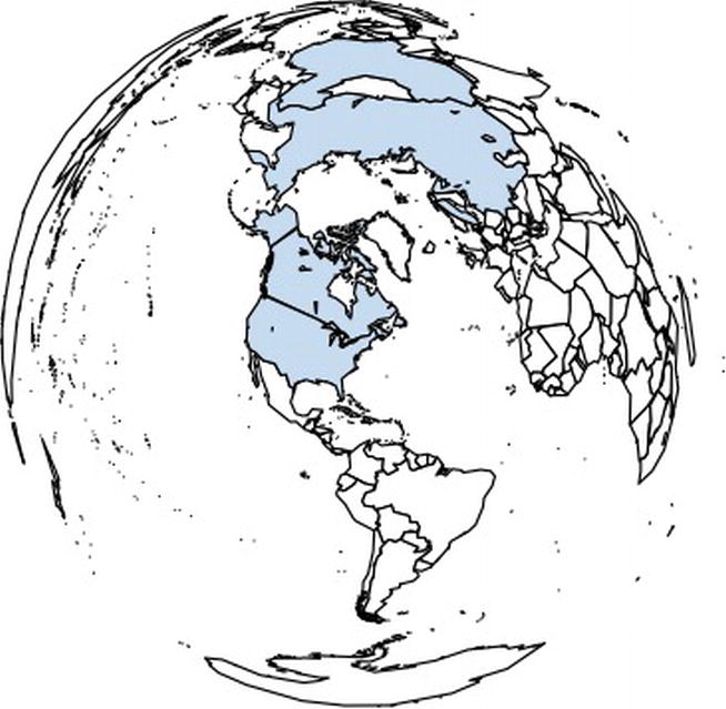
Figure 5-8. Data map using a world map
From this map we can see that the countries from our unique list are shaded blue and the rest of the countries are colored white. This is good, but we can make it better.
Adding Latitude and Longitude
Let’s start by adding latitude and longitude lines, which will accentuate the curvature of the globe and give context to where the poles are. To create latitude and longitude lines, we first create a new map object, but we will set plot to FALSE so that the map is not drawn to the screen. We’ll save this map object to a variable named m:
m <- map('world',plot=FALSE)
We’ll next call map.grid() and pass in our stored map object:
map.grid(m, col="blue", label=FALSE, lty=2, pretty=TRUE)
Note that if you are running this code line by line in the command window, it’s important to keep the Quartz graphic window open as you type the lines in so that R can update that chart. If you close the Quartz window while typing it in line by line, you could get an error stating that plot.new has not been called. Or you could type each line into a text file and copy them into the R command line all at once.
While we’re at it, let’s add a scale to the chart to show:
map.scale()
Our completed R code should now look like so:
library(maps)
library(mapproj)

logDataFile <- '/Applications/MAMP/htdocs/accessLogData.txt'
logColumns <- c("IP", "date", "HTTPstatus", "country", "state", "city")
logData <- read.table(logDataFile, sep=",", col.names=logColumns)

country <- unique(logData$country)
country <- sapply(country, function(countryCode){
  #trim whitespaces from the country code
  countryCode <- gsub("(^ +)|( +$)", "", countryCode)
  if(countryCode == "US"){
    countryCode<- "USA"
  }else if(countryCode == "CN"){
    countryCode<- "China"
  }else if(countryCode == "CA"){
    countryCode<- "Canada"
  }else if(countryCode == "SE"){
    countryCode<- "Sweden"
  }else if(countryCode == "UA"){
    countryCode<- "USSR"
  }
})


countryMatch <-  match.map("world", country)


#color code any states with visit data as light blue
colorCountry <- sapply(countryMatch, function(c){
 if(!is.na(c)) c <- "#C6DBEF"
 else c <- "#FFFFFF"
})


m <- map('world',plot=FALSE)
map('world',proj='azequalarea',orient=c(41,-74,0), boundary=TRUE, col=colorCountry,fill=TRUE)
map.grid(m,col="blue", label=FALSE, lty=2, pretty=TRUE)
map.scale()
And this code outputs the world map shown in Figure 5-9.
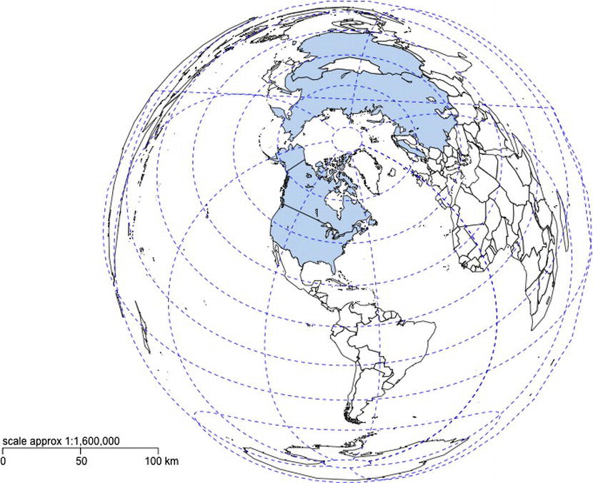
Figure 5-9. Globe data map with latitude and longitude lines as well as scale
Very nice! Next, let’s drill into a breakdown of visits by states in the United States.
Displaying Regional Data
Let’s start by isolating U.S. data; we can do this by selecting all rows in which the state does not equal “XX”. Remember setting the value in the state column to “XX” when we were parsing the access log in PHP? This is why. Countries other than the United States don’t have state data associated with them, so we can simply pull only the rows that have state data.
usData <- logData[logData$state != "XX", ]
We next need to replace the state abbreviations that we got from hostip.info with the full state names so that we can create a match.map lookup list, much like we did with the preceding country data.
The upside with state data is that R has a data set that contains all 50 U.S. state names, abbreviations, and even more esoteric information such as area of the state and named divisions (New England, Middle Atlantic, and so on). For more information, type ?state.name at the R console.
We can use the information in this data set to match the state abbreviations with the full state names that the map package needs. To do this, we use the apply() function to run an anonymous function that greps through the state.abb data set to find a match for the passed-in state abbreviation and then use that returned value as the index for retrieving the full state name from the state.name data set:
usData$state <- apply(as.matrix(usData$state), 1, function(s){
  #trim the abbreviation of whitespaces
  s <- gsub("(^ +)|( +$)", "", s)
  s <- state.name[grep(s, state.abb)]
})
We achieve the same functionality as the previous country match, but much more elegantly. If we were so inclined, we could go back and create our own data set of country names for future use to have a similar elegant solution for the country match.
Now that we have full state names to use, we can pull a unique list of state names and use that list to create a map matched list (again, just as we did for countries):
states <- unique(usData$state)
stateMatch <- match.map("state", states)
With our state match list, we can again apply a function to it that will look for matches in our match list, elements that do not have the value NA, and set the value for those elements to our nice light blue color while all elements that do have the value of NA get set to white. We save this list in a variable that we name colorMatch:
#color code any states with visit data as light blue
colorMatch <- sapply(stateMatch, function(s){
 if(!is.na(s)) s <- "#C6DBEF"
 else s <- "#FFFFFF"
})
We can then use colorMatch in our call to the map() function:
map("state", resolution = 0,lty = 0,projection = "azequalarea", col=colorMatch,fill=TRUE)
Hmm, but notice something? Only the colored areas are drawn to the stage, as shown in Figure 5-10.

Figure 5-10. Data map with only states that have data displayed
We need to make a second map() call that will draw the remainder of the map. In this map() call, we will set the add parameter to TRUE, which will cause the new map that we are drawing to be added to the current map. While we’re at it, let’s create a scale for this map as well:
map("state", col = "black", fill=FALSE, add=TRUE, lty=1, lwd=1, projection="azequalarea")
map.scale()
This code produces the finished state map in Figure 5-11.
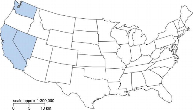
Figure 5-11. Completed state data map
Distributing the Visualization
OK, now let’s put our R code in an R Markdown file for distribution. Let’s go into RStudio and click File ➤ New ➤ R Markdown. Let’s add a header and make sure that our R code is wrapped in ```{r} tags and that our charts have heights and widths assigned to them. Our completed R Markdown file should look like this:
Visualizing Spatial Data from Access Logs
========================================================


```{r}
library(maps)
library(mapproj)

logDataFile <- '/Applications/MAMP/htdocs/accessLogData.txt'
logColumns <- c("IP", "date", "HTTPstatus", "country", "state", "city")
logData <- read.table(logDataFile, sep=",", col.names=logColumns)

```


```{r fig.width=15, fig.height=10}
#chart worldwide visit data


#unfortunately there is no state.name equivalent for countries so we must check
#the explicit country names. In the us states below we are able to accomplish this much
#more efficiently
country <- unique(logData$country)
country <- sapply(country, function(countryCode){
  #trim whitespaces from the country code
  countryCode <- gsub("(^ +)|( +$)", "", countryCode)
  if(countryCode == "US"){
    countryCode<- "USA"
  }else if(countryCode == "CN"){
    countryCode<- "China"
  }else if(countryCode == "CA"){
    countryCode<- "Canada"
  }else if(countryCode == "SE"){
    countryCode<- "Sweden"
  }else if(countryCode == "UA"){
    countryCode<- "USSR"
  }
})


countryMatch <-  match.map("world", country)

#color code any states with visit data as light blue
colorCountry <- sapply(countryMatch, function(c){
 if(!is.na(c)) c <- "#C6DBEF"
 else c <- "#FFFFFF"
})

m <- map('world',plot=FALSE)
map('world',proj='azequalarea',orient=c(41,-74,0), boundary=TRUE, col=colorCountry,fill=TRUE)
map.grid(m,col="blue", label=FALSE, lty=2, pretty=FALSE)
map.scale()

```


```{r fig.width=10, fig.height=7}
#isolate the US data, scrub any unknown states
usData <- logData[logData$state != "XX", ]
usData$state <- apply(as.matrix(usData$state), 1, function(s){
  #trim the abbreviation of whitespaces
  s <- gsub("(^ +)|( +$)", "", s)
  s <- state.name[grep(s, state.abb)]
})

s <- map('state',plot=FALSE)
states <- unique(usData$state)
stateMatch <- match.map("state", states)

#color code any states with visit data as light blue
colorMatch <- sapply(stateMatch, function(s){
 if(!is.na(s)) s <- "#C6DBEF"
 else s <- "#FFFFFF"
})


map("state", resolution = 0,lty = 0,projection = "azequalarea", col=colorMatch,fill=TRUE)
map("state", col = "black",fill=FALSE,add=TRUE,lty=1,lwd=1,projection="azequalarea")
map.scale()
```
This code produces the output shown in Figure 5-12. I have also made this R script publicly available at the following URL: http://rpubs.com/tomjbarker/3878.
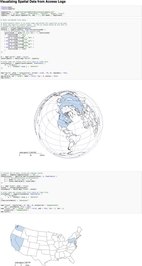
Figure 5-12. Data maps in RMarkdown
Summary
This chapter discussed parsing access logs to produce data map visualizations. You looked at both global country data in your maps as well as more localized state data. This is the first taste of how you can begin to bring usage data to life.
The next chapter looks at bug backlog data in the context of time series charts.