![]()
A Deeper Dive into R
The last chapter explored some introductory concepts in R, from using the console to importing data. We installed packages and discussed data types, including different list types. We finished up by talking about functions and creating closures.
This chapter will look at object-oriented concepts in R, explore concepts in statistical analysis, and finally see how R can be incorporated into R Markdown for real time distribution.
Object-Oriented Programming in R
R supports two different systems for creating objects: the S3 and S4 methods. S3 is the default way that objects are handled in R. We’ve been using and making S3 objects with everything that we’ve done so far. S4 is a newer way to create objects in R that has more built-in validation, but more overhead. Let’s take a look at both methods.
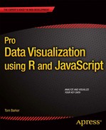
Okay, so traditional, class-based, object-oriented design is characterized by creating classes that are the blueprint for instantiated objects (see Figure 3-1).
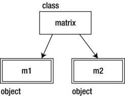
Figure 3-1. The matrix class is used to create the variables m1 and m2, both matrices
At a very high level, in traditional object-oriented languages, classes can extend other classes to inherit the parent class’ behavior, and classes can also implement interfaces, which are contracts defining what the public signature of the object should be. See Figure 3-2 for an example of this, in which we create an IUser interface that describes what the public interface should be for any user type class, and a BaseUser class that implements the interface and provides a base functionality. In some languages, we might make BaseUser an abstract class, a class that can be extended but not directly instantiated. The User and SuperUser classes extend BaseClass and customize the existing functionality for their own purposes.
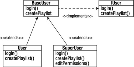
Figure 3-2. An IUser interface implemented by a superclass BaseUser that the subclasses User and SuperUser extend
There also exists the concept of polymorphism, in which we can change functionality via the inheritance chain. Specifically, we would inherit a function from a base class but override it, keep the signature (the function name, the type and amount of parameters it accepts, and the type of data that it returns) the same, but change what the function does. Compare overriding a function to the contrasting concept of overloading a function, in which the function would have the same name but a different signature and functionality.
S3, so called because it was first implemented in version 3 of the S language, uses a concept called generic functions. Everything in R is an object, and each object has a string property called class that signifies what the object is. There is no validation around it, and we can overwrite the class property ad hoc. That’s the main problem with S3—the lack of validation. If you ever had an esoteric error message returned when trying to use a function, you probably experienced the repercussions of this lack of validation firsthand. The error message was probably generated not from R detecting that an incorrect type had been passed in, but from the function trying to execute with what was passed in and failing at some step along the way.
See the following code, in which we create a matrix and change its class to be a vector:
> m <- matrix(c(1:10), nrow=2)
> m
   [,1] [,2] [,3] [,4] [,5]
[1,]    1    3    5    7    9
[2,]    2    4    6    8   10
> class(m) <- "vector"
> m
   [,1] [,2] [,3] [,4] [,5]
[1,]    1    3    5    7    9
[2,]    2    4    6    8   10
attr(,"class")
[1] "vector"
Generic functions are objects that check the class property of objects passed into them and exhibit different behavior based on that attribute. It’s a nice way to implement polymorphism. We can see the methods that a generic function uses by passing the generic function to the methods() function. The following code shows the methods of the plot() generic function:
> methods(plot)
[1] plot.acf*           plot.data.frame*    plot.decomposed.ts* plot.default        plot.dendrogram*
[6] plot.density        plot.ecdf           plot.factor*        plot.formula*       plot.function
[11] plot.hclust*        plot.histogram*     plot.HoltWinters*   plot.isoreg*        plot.lm
[16] plot.medpolish*     plot.mlm            plot.ppr*           plot.prcomp*        plot.princomp*
[21] plot.profile.nls*   plot.spec           plot.stepfun        plot.stl*           plot.table*
[26] plot.ts             plot.tskernel*      plot.TukeyHSD
Non-visible functions are asterisked
Notice that within the generic plot() function is a myriad of methods to handle all the different types of data that could be passed to it, such as plot.data.frame for when we pass a data frame to plot(); or if we want to plot a TukeyHSD object plot(), plot.TukeyHSD is ready for us.
![]() Note Type ?TukeyHSD for more information on this object.
Note Type ?TukeyHSD for more information on this object.
Now that you know how S3 object-oriented concepts work in R, let’s see how to create our own custom S3 objects and generic functions.
An S3 class is a list of properties and functions with an attribute named class. The class attribute tells generic functions how to treat objects that implement a particular class. Let’s create an example using the UserClass idea from Figure 3-2:
> tom <- list(userid = "tbarker", password = "password123", playlist=c(12,332,45))
> class(tom) <- "user"
We can inspect our new object by using the attributes() function, which tells us the properties that the object has as well as its class:
> attributes(tom)
$names
[1] "userid"   "password" "playlist"
$class
[1] "user"
Now to create generic functions that we can use with our new class. Start by creating a function that will handle only our user object; then generalize it so any class can use it. It will be the createPlaylist() function and it will accept the user on which to perform the operation and a playlist to set. The syntax for this is [ function name ].[ class name ]. Note that we access the properties of S3 objects using the dollar sign:
>createPlaylist.user <- function(user, playlist=NULL){
    user$playlist <- playlist
    return(user)
}
Note that while you type directly into the console, R enables you to span several lines without executing your input until you complete an expression. After your expression is complete, it will be interpreted. If you want to execute several expressions at once, you can copy and paste into the command line.
Let’s test it to make sure it works as desired. It should set the playlist property of the passed-in object to the vector that is passed in:
> tom <- createPlaylist.user(tom, c(11,12))
> tom
$userid
[1] "tbarker"

$password
[1] "password123"

$playlist
[1] 11 12

attr(,"class")
[1] "user"
Excellent! Now let’s generalize the createPlaylist() function to be a generic function. To do this, we just create a function named createPlaylist and have it accept an object and a value. Within our function, we use the UseMethod() function to delegate functionality to our class-specific createPlaylist() function: createPlaylist.user.
The UseMethod() function is the core of generic functions: it evaluates the object, determines its class, and dispatches to the correct class-specific function:
> createPlaylist <- function(object, value)
{
      UseMethod("createPlaylist", object)
}
Now let’s try it out to see whether it worked:
> tom <- createPlaylist(tom, c(21,31))
> tom
$userid
[1] "tbarker"

$password
[1] "password123"

$playlist
[1] 21 31

attr(,"class")
[1] "user"
Excellent!
Let’s look at S4 objects. Remember that the main complaint about S3 is the lack of validation. S4 addresses this lack by having overhead built into the class structure. Let’s take a look.
First we’ll create the user class. We do this with the setClass() function.
- The first parameter in the setClass() function is a string that signifies the name of the class that we are creating.
- The next parameter is called representation and it is a list of named properties.
setClass("user",
representation(userid="character",
    password="character",
    playlist="vector"
)
)
We can test it by creating a new object from this class. We use the new() function to create a new instance of the class:
> lynn <- new("user", userid="lynn", password="test", playlist=c(1,2))
> lynn
An object of class "user"
Slot "userid":
[1] "lynn"

Slot "password":
[1] "test"

Slot "playlist":
[1] 1 2
Very nice. Note that for S4 objects, we use the @ symbol to reference properties of objects:
> lynn@playlist
[1] 1 2
> class(lynn)
[1] "user"
attr(,"package")
[1] ".GlobalEnv
Let’s create a generic function for this class by using the setMethod() function. We simply pass in the function name, the class name, and then an anonymous function that will serve as the generic function:
> setMethod("createPlaylist", "user", function(object, value){
      object@playlist <- value
      return(object)
 })
Creating a generic function from function 'createPlaylist' in the global environment
[1] "createPlaylist"
>
Let’s try it out:
> lynn <- createPlaylist(lynn, c(1001, 400))
> lynn
An object of class "user"
Slot "userid":
[1] "lynn"

Slot "password":
[1] "test"

Slot "playlist":
[1] 1001  400
Excellent!
Although some prefer the simplicity and flexibility of the S3 way, some prefer the structure of the S4 method; the choice of S3 or S4 objects is purely one of personal preference. My own preference is for the simplicity of S3, and that is what we will be using for the remainder of the book. Google, in its R Style Guide available at http://google-styleguide.googlecode.com/svn/trunk/google-r-style.html, mirrors my own feelings about S3, saying “Use S3 objects and methods unless there is a strong reason to use S4 objects or methods.”
Statistical Analysis with Descriptive Metrics in R
Now let’s take a look at some concepts in statistical analysis and how to implement them in R. You might remember most of the concepts covered in this chapter from an introductory statistics class from college; they are the base concepts needed to begin to think about and discuss your data.
First, let’s get some data on which we’ll perform statistical analysis. R comes preloaded with a number of data sets that we can use as sample data. To see a list of available data sets with your install simply type data() at the console. You’ll be presented with the screen that you see in Figure 3-3.
Figure 3-3. Available data sets in R
To see the contents of a data set, you can call it by name in the console. Let’s take a look at the USArrests data set, which we’ll use for the next few topics.
> USArrests
                Murder  Assault   UrbanPop Rape
Alabama          13.2    236       58      21.2
Alaska           10.0    263       48      44.5
Arizona           8.1    294       80      31.0
Arkansas          8.8    190       50      19.5
California        9.0     276       91     40.6
Colorado          7.9     204       78     38.7
Connecticut       3.3     110       77     11.1
Delaware          5.9     238       72     15.8
Florida          15.4     335       80     31.9
Georgia          17.4     211       60     25.8
Hawaii            5.3      46       83     20.2
Idaho             2.6     120       54     14.2
Illinois         10.4     249       83     24.0
Indiana           7.2     113       65     21.0
Iowa              2.2      56       57     11.3
Kansas            6.0     115       66     18.0
Kentucky          9.7     109       52     16.3
Louisiana        15.4     249       66     22.2
Maine             2.1      83       51      7.8
Maryland         11.3     300       67     27.8
Massachusetts     4.4     149       85     16.3
Michigan         12.1     255       74     35.1
Minnesota         2.7      72       66     14.9
Mississippi      16.1     259       44     17.1
Missouri          9.0     178       70     28.2
Montana           6.0     109       53     16.4
Nebraska          4.3     102       62     16.5
Nevada           12.2     252       81     46.0
New Hampshire     2.1      57       56      9.5
New Jersey        7.4     159       89     18.8
New Mexico       11.4     285       70     32.1
New York         11.1     254       86     26.1
North Carolina   13.0     337       45     16.1
North Dakota      0.8      45       44      7.3
Ohio              7.3     120       75     21.4
Oklahoma          6.6     151       68     20.0
Oregon            4.9     159       67     29.3
Pennsylvania      6.3     106       72     14.9
Rhode Island      3.4     174       87      8.3
South Carolina   14.4     279       48     22.5
South Dakota      3.8      86       45     12.8
Tennessee        13.2     188       59     26.9
Texas            12.7     201       80     25.5
Utah              3.2     120       80     22.9
Vermont           2.2      48       32     11.2
Virginia          8.5     156       63     20.7
Washington        4.0     145       73     26.2
West Virginia     5.7      81       39      9.3
Wisconsin         2.6      53       66     10.8
Wyoming           6.8     161       60     15.6
>
The first function in R that we’ll look at is the summary() function, which accepts an object and returns the following key descriptive metrics, grouped by column:
- minimum value
- maximum value
- median for numbers and frequency for strings
- mean
- first quartile
- third quartile
Let’s run the USArrests data set through the summary() function:
> summary(USArrests)
   Murder          Assault         UrbanPop          Rape
Min.   : 0.800   Min.   : 45.0   Min.   :32.00   Min.   : 7.30
1st Qu.: 4.075   1st Qu.:109.0   1st Qu.:54.50   1st Qu.:15.07
Median : 7.250   Median :159.0   Median :66.00   Median :20.10
Mean   : 7.788   Mean   :170.8   Mean   :65.54   Mean   :21.23
3rd Qu.:11.250   3rd Qu.:249.0   3rd Qu.:77.75   3rd Qu.:26.18
Max.   :17.400   Max.   :337.0   Max.   :91.00   Max.   :46.00
Let’s look at each of these metrics in detail, as well as the standard deviation.
Median and Mean
Note that the median is the number that is the middle value in a data set, quite literally the number that has the same amount of numbers greater and less than itself in the data set. If our data set looks like the following, the median is 3:
1, 2, 3, 4, 5
But notice that it’s easy to find the median when there are an odd number of items in a data set. Suppose that there is an even number of items in a data set, as follows:
1, 2, 3, 4, 5, 6
In this case we take the middle pair, 3 and 4, and get the average of those two numbers. The median is 3.5.
Why does the median matter? When you look at a data set, there are usually outliers at either end of the spectrum, values that are much higher or much lower than the rest of the data set. Gathering the median value excludes these outliers, giving a much more realistic view of the average values.
Contrast this idea with the mean, which is simply the sum of the values in a data set divided by the number of items. The values include the outliers, so the mean can be skewed by having significant outliers and really represent the full data set.
For example, look at the following data set:
1, 2, 3, 4, 30
The median is still 3 for this data set, but the mean is 8, because of this:
median = [1,2]3[4,30]
mean =  1 + 2 + 3 + 4 + 30 = 40
    40 / 5 = 8
Quartiles
The median is the center of the data set, which means that the median is the second quartile. Quartiles are the points that divide a data set into four even sections. We can use the quantile() function to pull just the quartiles from our data set.
> quantile(USArrests$Murder)
  0%    25%    50%    75%   100%
0.800  4.075  7.250 11.250 17.400
The summary() function simply returns the quartiles, as well as the minimum, maximum, and mean values. Here are the summary() results for comparison, with the previous quartiles highlighted:
> summary(USArrests)
   Murder          Assault         UrbanPop          Rape
Min.   : 0.800   Min.   : 45.0   Min.   :32.00   Min.   : 7.30
1st Qu.: 4.075   1st Qu.:109.0   1st Qu.:54.50   1st Qu.:15.07
Median : 7.250   Median :159.0   Median :66.00   Median :20.10
Mean   : 7.788   Mean   :170.8   Mean   :65.54   Mean   :21.23
3rd Qu.:11.250   3rd Qu.:249.0   3rd Qu.:77.75   3rd Qu.:26.18
Max.   :17.400   Max.   :337.0   Max.   :91.00   Max.   :46.00
Standard Deviation
Speaking of the idea of the mean, there is also the idea that data has a normal distribution, or that data is normally densely clustered around the mean with lighter groupings above and below the mean. This is usually demonstrated with a bell curve, in which the mean is the top of the curve, and the outliers are distributed on either end of it (see Figure 3-4).
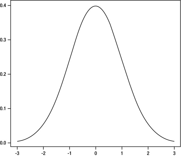
Figure 3-4. The bell curve of a normal distribution
Standard deviation is a unit of measurement that describes the average of how far apart the data is distributed from the mean, so we can detail how far each data point is from the mean in terms of standard deviations.
In R, we can determine the standard deviation using the sd() function. The sd() function expects a vector of numeric values:
> sd(USArrests$Murder)
[1] 4.35551
If we want to gather the standard deviation for a matrix we can use the apply() function to apply the sd() function, like so:
> apply(USArrests, sd)
  Murder    Assault   UrbanPop       Rape murderRank
4.355510  83.337661  14.474763   9.366385  14.574930
RStudio IDE
If you prefer to develop in an integrated development environment (IDE) instead of at the command line, you can use a free product called RStudio IDE. The RStudio IDE is made by the RStudio company, and is much more than just an IDE (as you will soon see). The RStudio company was founded by JJ Allaire, creator of ColdFusion. RStudio IDE is available for download at http://www.rstudio.com/ide/ (see Figure 3-5 for a screen shot of the download page).
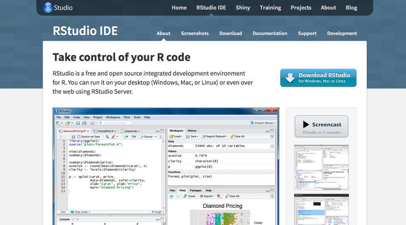
Figure 3-5. RStudio IDE homepage
![]() Note You should install the RStudio IDE now because you will use it in the remainder of this chapter.
Note You should install the RStudio IDE now because you will use it in the remainder of this chapter.
After installation, the IDE is split into four panes (see Figure 3-6).
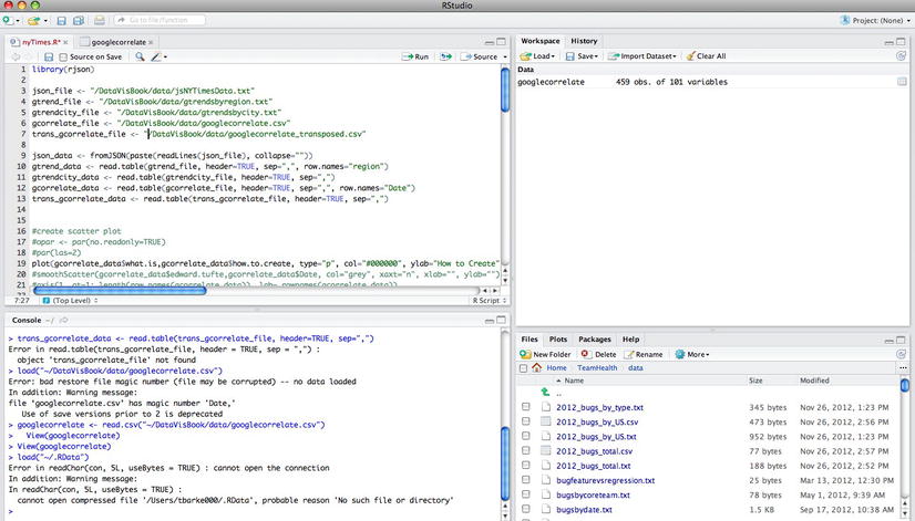
Figure 3-6. Caption
The upper-left pane is the R script file in which we edit our R source code. The bottom-left pane is the R command line. The upper-right side pane holds the command history as well as all the objects in our current workspace. The bottom-right pane is split into tabs that can show the following:
- Contents of the file system for the current working directory
- Plots or charts that have been generated
- Current packages installed
- R help pages
Although it is great to have everything that you need in one place, here is where things become really interesting.
R Markdown
In version 0.96 of RStudio, the team announced support for R Markdown using the knitr package. We can now embed R code into markdown documents that can get interpreted by knitr into HTML. But it gets even better.
The RStudio company also makes a product called RPubs that allows users to create accounts and host their R markdown files for distribution over the Web.
![]() Note Markdown is a plain text markup language created by John Gruber and Aaron Swartz. In markdown, you can use simple and lightweight text encodings to signify formatting. The markdown document is read and interpreted and an HTML file is output.
Note Markdown is a plain text markup language created by John Gruber and Aaron Swartz. In markdown, you can use simple and lightweight text encodings to signify formatting. The markdown document is read and interpreted and an HTML file is output.
A quick overview of markdown syntax follows:
header 1
=========
header 2
--------------
###header 3
####header 4
*italic*
**bold**
[link text]([URL])

The great thing about R Markdown is that we can embed R code within our markdown document. We embed R using three tick marks and the letter r in curly braces:
```{r}
[R code]
```
We need three things to begin creating R Markdown (.rmd) documents:
- R
- R Studio IDE version 0.96 or higher
- The knitr package
The knitr package is used to reformat R into several different output formats, including HTML, markdown, or even plain text.
![]() Note Information about the knitr package is available at http://yihui.name/knitr/.
Note Information about the knitr package is available at http://yihui.name/knitr/.
Because you already have R and RStudio IDE installed, you will first install knitr. R Studio IDE has a nice interface to install packages: simply go to the Tools file menu and click Install Packages. You should see the popup that shown in Figure 3-7, in which you can specify the package name (R Studio IDE has a nice type ahead here for package discovery) and what library to install to.
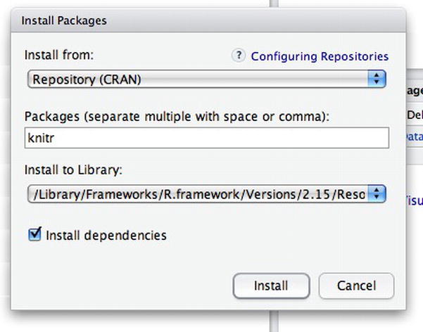
Figure 3-7. Installing the knitr package
After knitr is installed, you need to close and relaunch RStudio IDE. You then go to the File menu and choose File ➤ New, in which you should see a number of options, including R Markdown. If you choose R Markdown, you get a new file with the template shown in Figure 3-8.
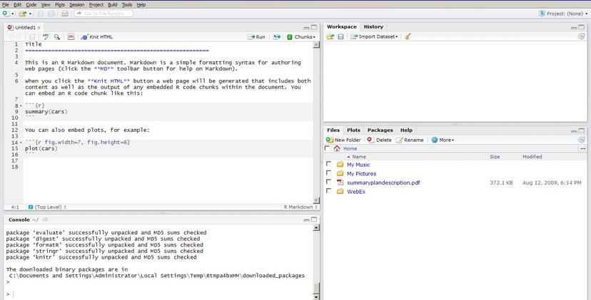
Figure 3-8. RStudio IDE
The R Markdown template has the following code:
Title
========================================================
This is an R Markdown document. Markdown is a simple formatting syntax for authoring web pages (click the **MD** toolbar button for help on Markdown).
When you click the **Knit HTML** button a web page will be generated that includes both content as well as the output of any embedded R code chunks within the document. You can embed an R code chunk like this:
```{r}
summary(cars)
```

You can also embed plots, for example:

```{r fig.width=7, fig.height=6}
plot(cars)
```
This is the template, and when you click the Knit HTML button you will see the output shown in Figure 3-9.
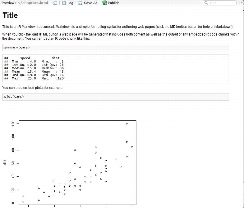
Figure 3-9. HTML output of RMarkdown template
Did you notice the Publish button at the top of Figure 3-9? That is how we push our R Markdown file to RPubs for hosting and distribution over the Web.
RPubs
RPubs is a free web publishing platform for R Markdown files, provided by RStudio (the company). You can create a free account by visiting http://www.rpubs.com. Figure 3-10 shows a screen shot of the RPubs homepage.
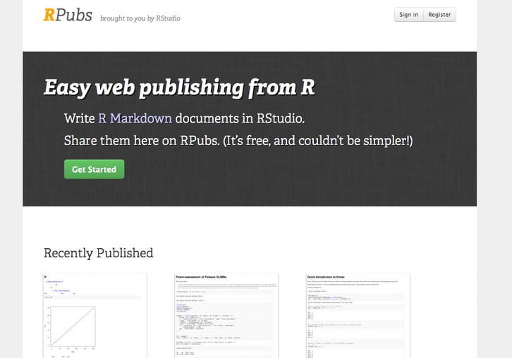
Figure 3-10. RPubs homepage
Just click the Register button and fill out the form to create your free account. RPubs is fantastic; it’s a platform in which we can post our R Markdown documents for distribution.
![]() Caution Be aware that every file you put up on RPubs is publicly available, so be sure not to put any sensitive or proprietary information in it. If you don’t want to put your R Markdown files where they are available for the whole world to see, you can instead click the Save As button right next to the Publish button to save the file as regular HTML.
Caution Be aware that every file you put up on RPubs is publicly available, so be sure not to put any sensitive or proprietary information in it. If you don’t want to put your R Markdown files where they are available for the whole world to see, you can instead click the Save As button right next to the Publish button to save the file as regular HTML.
After you click the Publish button, you are prompted to log in with your RPubs account. After logging in, you will be directed to the Document Details page, as seen in Figure 3-11.
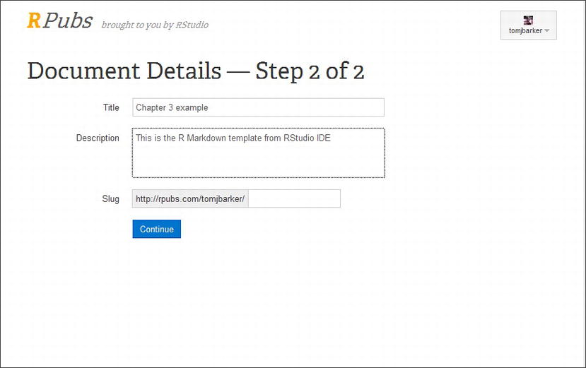
Figure 3-11. Publishing to RPubs
After filling out the document details, a title for your document, and a description, you will be directed to your document hosted in RPubs. See Figure 3-12 for the template from Figure 3-9 hosted in RPubs and available publicly here: http://www.rpubs.com/tomjbarker/3370.
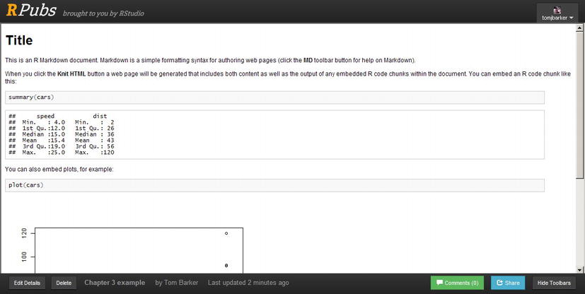
Figure 3-12. RMarkdown template published to RPubs
This is a powerful distribution method for R documents and for communicating data visualizations. In the coming chapters, we will put all the completed R charts up on RPubs for public consumption.
Summary
This chapter explored some deeper concepts in R, from the different models of object-oriented design available, to how to do statistical analysis with R. We even looked at how to use RMarkdown and RPubs to make data visualizations in R available for public distribution.
In the next chapter, we will look at D3, a JavaScript library that enables us to analyze and visualize data within the browser and add interactivity to visualizations.