7
ETL into a Market Basket Datamart
The purpose of the Market Basket Extract, Transform, and Load (ETL) application is specifically to populate a Market Basket BI Table. If a Market Basket application includes the Analysis branch shown in Figure 6.1, then an ETL application populates data in a set of Market Basket tables that are dedicated to the Analysis branch. If a Market Basket application includes the Reporting branch shown in Figure 6.2, then an ETL application populates data in a set of Market Basket tables that are dedicated to the Reporting branch. For every set of Market Basket Analysis tables, a set of ETL applications populates those tables. For every set of Market Basket Reporting tables, a separate set of ETL applications populates those tables as well. The number of Market Basket ETL applications equals the number of sets of Market Basket tables.
Requirement: Populate the Market Basket BI Table
The first requirement of the Market Basket ETL is to extract data from the data warehouse and load that data in the Market Basket BI Table. This requirement may sound rather simple, but it is not. Although it may seem that this requirement can be met by a SELECT statement that writes data to an extract file, and then an INSERT statement that loads the data in the extract file, an ETL application is not quite that simple. To avoid “garbage out,” an ETL application must avoid “garbage in.” To avoid “garbage in,” an ETL application must include safeguards to protect the data, and therefore the Market Basket application that will use the data.
Singularity
Each Itemset must be represented once, and only once. This is a basic requirement of every ETL application. The initial extract application of an ETL application must be able to recognize when it has, and has not, encountered a set of data before. Data coming from an OLTP system can be rather tricky that way. Fortunately, however, a data warehouse presents a much more stable and controlled data source. Regardless, extracting data from a data warehouse is not time to relax on this, the most basic of ETL requirements. The Market Basket ETL application that extracts data from the data warehouse must be able to control the data such that each set of data and each row of data are allowed to pass through to the Market Basket Table only once.
Completeness
Each Itemset must be complete. This is another basic requirement of every ETL application. A set of data must be complete such that a set of data is a complete set of data, not a partial set of data. The goal of this requirement is to meet the expectation of the analysts. The expectation of analysts is a subtle, yet not quite so subtle, requirement. Analysts have the expectation that the data in an Itemset is, unless otherwise posted, a full complement of the data in that Itemset.
Date—If a set of data represents all the Itemsets that happened on a specific date, then analysts assume that date is fully represented within that set of Itemsets. All rows of data associated with a date are presented with that date. All rows of data not associated with a date are not presented with that date. Therefore, if an analyst is looking for an Itemset, and does not see that Itemset on a specific date, the analyst does not see it on that date because it did not occur on that date. An analyst can operate with this assumption because the data is complete for that date.
Objects—The set of objects in an Itemset is all the objects that occurred in that Itemset. If an object is not listed within an Itemset, it is not there because it did not occur within that Itemset. Therefore, if an analyst is looking for an object, and does not see it within an Itemset, the analyst does not see it there because it did not occur within that Itemset. An analyst can operate with this assumption because the data is complete for that Itemset.
An analyst cannot analyze data that is not there. Also, analysts tend to get rather upset when they publish conclusions based on data and then need to revise those conclusions because apparent gaps in that data have been filled in by additional data that led to different conclusions. That sort of behavior does not inspire confidence in a data warehouse or a Market Basket application. To that end, it would be better to delay releasing a set of data in the Market Basket application until that data is complete than to publish an incomplete set of data.
Yes, it is technically feasible to provide metadata that would tell the Market Basket analysts which data is incomplete and what exactly about that data is incomplete. It is also technically feasible to design and deliver a user interface for analysis that would leverage such metadata. That would be an advanced use of metadata for the Completeness requirement. If your data warehouse has such an advanced use of metadata, then you most probably did not continue reading this section on the Completeness requirement down to this paragraph. That being the case, you should accept the “all or nothing” form of the Completeness requirement, such that every set of data in your Market Basket application is complete without any gaps.
Identity
Each group of data must be uniquely identifiable. Each Itemset must be uniquely identifiable within a group of data. Each row of data must be uniquely identifiable within an Itemset.
No, the analysts will not perform any analysis on the unique identifiers of the groups, Itemsets, or rows of data. To that end, the analysts should never be aware of the unique identifiers of the groups, Itemsets, or rows of data. The audience of this requirement is the ETL application, not the analysts.
After a Market Basket application gets busy, the Market Basket ETL application will have multiple iterations of ETL occurring simultaneously. So, the ETL application cannot assume one and only one iteration of ETL will occur at a moment in time. In that way, an ETL can become a victim of its own success. The answer to that problem is control. An ETL application must be able to control each phase of each iteration of ETL individually, and separately from all the other phases and iterations of ETL. The key to such a level of control is the ability to uniquely identify each and every group of data, Itemset, and row.
This requirement does not mean that the ETL application must maintain a mirror image of the data for every unique identifier. That would mean a mirror image for every row, another mirror image for every Itemset, and another mirror image for every group. This requirement is not about maintaining mirror images of data. Rather, this requirement is about the ability to know what the ETL has done, is doing, and has yet to do. To maintain that level of control, an ETL application needs handles or name tags for the groupings of data. That way, an ETL application can maintain a log of groups of data. By looking in a group of data the ETL application can see all the unique identifiers of the Itemsets, and if necessary, all the unique identifiers of the rows.
That log of ETL activity will eventually become very important in the defense of the ETL application. The day will soon come when an analyst will need to know what data was in the Market Basket application and what data had not yet arrived in the Market Basket application as of a moment in time. That is when the log of ETL activity will become very, very handy. That is also when the ability to tie every row of every Itemset of every group of data back to an ETL activity at a moment in time will become very, very necessary.
Metadata
Metadata comes in two forms: Static Metadata and Dynamic Metadata. Static Metadata is the descriptions and definitions of the structures of the data warehouse and the processes of the ETL application. Static Metadata answers the “What is that?” questions of a data warehouse. Dynamic Metadata is the log of the activities of the ETL application as it populates the data warehouse. Dynamic Metadata answers the “What happened?” questions of a data warehouse.
This is true for all ETL applications, including those that populate a data warehouse and those that populate a Market Basket application. For that reason, the ETL application that populates the data warehouse from which the Market Basket application gets its data may already have established Metadata structures (i.e., log tables) and processes (i.e., logging methods). If that is the case, then the already established ETL structures and processes that are used by the ETL application that populates the data warehouse should also be used by the ETL application that populates the Market Basket application.
If, however, a data warehouse ETL application does not already have Metadata structures and processes already created and operating within the data warehouse ETL, the Market Basket ETL application will have to create those structures and processes for itself. This would actually be a reasonable cause to pause the creation of a Market Basket ETL application until the construction of the data warehouse ETL Metadata structures and processes is complete. The level of confidence in the completeness and identity of the data within the Market Basket ETL application is in large part based on the completeness and identity of the data in the data warehouse ETL. If the data warehouse ETL is not able to guarantee the completeness and identity of its data, then the Market Basket ETL application will most probably not be able to guarantee the completeness and identity of the data it delivers to the Market Basket application.
Data Quality
Data quality is assessed by one of two methods: looking for something that should be there, or looking for something that should not be there. The “looking for something that should be there” method programmatically calculates the interrelationships within the data (e.g., Summed detail rows should equal header rows, units multiplied by unit price should equal total price) and posts an alert when the expected condition has not occurred. The “looking for something that should not be there” method programmatically looks for data that is obviously wrong (e.g., negative unit price, null values, alpha characters in a numeric field) and posts an alert when the unexpected condition has occurred. As the data was extracted from the original source, transformed in the ETL application, and then loaded into the data warehouse, that data should have gone through a data quality assessment.
If the data did indeed go through a data quality assessment on its way to the data warehouse, then the guarantees provided by those data quality assessments extend to the data in the data warehouse and now to the data coming from the data warehouse to the Market Basket application. Even if that is true, the Market Basket ETL application may need to include its own data quality assessments. The analysis of the data in the Market Basket application may expose, or assume, data behaviors or data interrelationships that are not already guaranteed by the data warehouse ETL. If that is the case, then the Market Basket ETL application will need to assess the data from the data warehouse in the Market Basket ETL application.
If the data did not go through a data quality assessment on its way into the data warehouse, then the Market Basket ETL must provide all the guarantees for all the data that comes from the data warehouse to the Market Basket application. Either way, the data quality methods are the same. The only difference is the inclusion of specific data quality assessments, which will lead to specific data quality guarantees.
If the data warehouse ETL does not already assess the quality of the data on its way to the data warehouse, that would be another reasonable cause to pause the creation of the Market Basket ETL until the data warehouse ETL has included data quality assessments in its processes. This may seem rather picky, but it is not. The time and energy expended in guaranteeing the data quality within the data warehouse should be directly associated with the data warehouse and not the Market Basket application. If that time and energy expenditure to create data quality assessments in the data warehouse is associated with the Market Basket application, it will diminish the perceived ROI and the Market Basket application and increase the perceived responsibilities of the Market Basket ETL. In that situation, the Market Basket ETL will be perceived to be the consumer and owner of the data warehouse ETL. While that may be true insofar as the human team members for the data warehouse and the Market Basket ETL may indeed be the same persons, in terms of management’s perception of budgets, roles, and responsibilities, the Market Basket application can only be best served by incurring only those expenses directly associated with the Market Basket application and owning only those responsibilities directly achieved by the Market Basket ETL.
Market Basket ETL Design
ETL is often thought to be an application, or set of applications, that retrieves data from an operational source system, conforms it to the design of a data warehouse, and then loads that conformed data into the data warehouse. So, it may seem strange to think of ETL as a set of applications that pull data from a data warehouse, conform that data to the design of a Market Basket application (or any other datamart), and then load that data into the Market Basket application (or, again, any other datamart). But, in the world of data warehousing, that is exactly what happens. ETL is a generalized name given to applications that move data in a controlled and intelligent fashion from a source platform to a destination platform.
Typically, ETL pulls data from a data warehouse and loads that data into a separate datamart for one of two primary reasons. The first reason is the separation of resource consumption. Architecturally, a data warehouse is a large data store with many customers. If a specific group of customers or application requires query response times and access patterns that will contend with the “large data store” design of a data warehouse and/or the other customers, a datamart allows that group or application to have clear and unchallenged access to the data they require. The second reason is the separation of structure designs. If a specific group or application requires that the data be provided in a structural design that is not conducive to the other customers of the data warehouse (and, yes, the Market Basket BI Table is not conducive to the other customers of a data warehouse), a datamart allows that group or application to have data in the structural design they require.
In the context of a Market Basket application, the Market Basket BI Table is a datamart that allows the Market Basket analysts to have their data in a form that is conducive to Market Basket Analysis. The Market Basket ETL application pulls data from the data warehouse, conforms it to the design of the Market Basket BI Table, and then loads that data into the Market Basket BI Table. Data in the Market Basket BI Table is then available for analysis. The Market Basket ETL application is, therefore, a datamart specifically designed for the purpose of Market Basket Analysis, which is populated by the Market Basket ETL application.
Unless a value-adding, ROI-generating requirement compels the use of real-time ETL, typically ETL applications are batch applications. Even then, real-time ETL is used only for tactical data that is sensitive to the immediate delivery of data from a source system. Market Basket analysts are looking at the data strategically, not tactically. The search for broad patterns over long periods of time is by definition strategic in nature. For that reason, Market Basket ETL is a batch ETL application. So, the first design decision of a Market Basket ETL application is that Market Basket ETL is a batch, not a real-time, application.
Step 1: Extract from a Fact Table and Load to a Market Basket Table
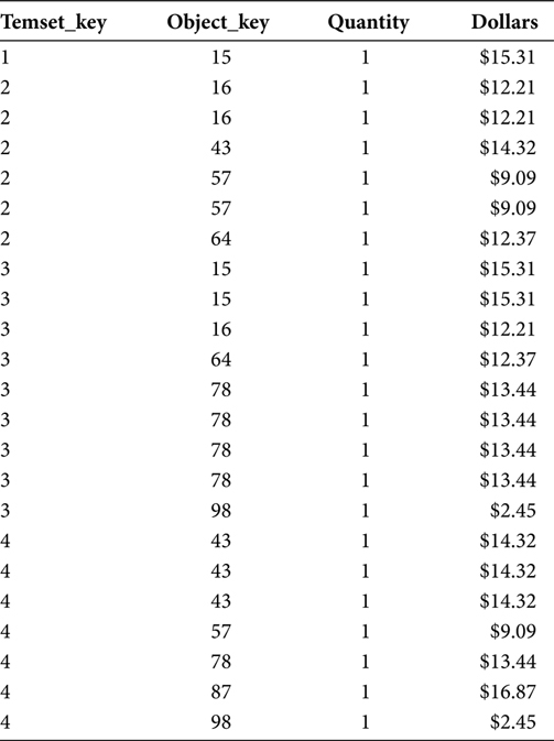
The source data for a Market Basket application is a Fact table in a data warehouse. That Fact table may contain sales transactions at a retail store, dinner receipts from a restaurant, work orders from a service provider, or click streams from an online retailer. Because the source table is a Fact table from the data warehouse, the Market Basket application can trust the quality of the data in that Fact table. If the quality of the data in the Fact table is not trustworthy, then the quality of the data in the data warehouse should be addressed before the Market Basket Analysis can begin.
A very small sample Fact table is shown in Table 7.1. The data in Table 7.1 will be the source of the sample tables in the remainder of this chapter.
TABLE 7.1
Fact Table
The first operation of the Market Basket ETL application is the extract from the Fact table and load into the Market Basket Table. Figure 7.1 shows this as one operation. A mature ETL application will assess the quality of the data as it passes by. While the Market Basket ETL application has some level of trust in the source Fact table, data quality assessments still provide some confidence that the Market Basket ETL application has maintained the quality and integrity of the data as it passes through the Market Basket ETL application. Chapters 8 and 9 of Building and Maintaining a Data Warehouse explain methods by which metadata and data quality work together to warranty data as it passes through an ETL application.
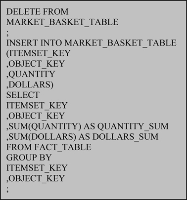
FIGURE 7.1
Load Market Basket Table.
At the end of this initial step, the Market Basket Table will contain a set of rows for every Itemset. Each Itemset will be uniquely identified by its Itemset_Key. The Itemset_Key in Table 7.2 is a single sequential numeric value. This numeric key structure may not be true in your data warehouse and your Market Basket application.
The Itemset_Key is defined by its role and purpose, not by its structure. An Itemset_Key must uniquely identify each and every individual transaction such that each and every transaction has one and only one Itemset_Key, and each and every Itemset_Key has one and only one transaction. The Itemset_Key can never repeat for another transaction. The Itemset_Key can include, and usually is, a compound key including a date. The inclusion of a date in the Itemset_Key means the Itemset_Key, sans the date portion, must be unique only within a twenty-four-hour period, rather than all of eternity. Twenty-four hours is a much more manageable span of time. So, frequently the date is included in the Itemset_Key. As explained in Chapter 5, date and time are often included in the Itemset_Key as they allow the analyst to stratify the data in a Market Basket Analysis application.
TABLE 7.2
Market Basket Table
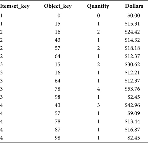
Two transformations to the data in an Itemset occur in this step. The first step is for the case of the Single Object Itemset. If an Itemset includes only one object, this step will add a “mirror” row of data for the same Itemset_Key, but with zero in the Object_Key and numeric metric columns (i.e., Quantity and Dollars). The reason for this addition to the data extracted from the Fact table is that in the recursive join, which will happen in the next step, every Itemset must have a second row with which it can join. In the case of a Single Object Itemset, that second row must be manufactured by the Market Basket ETL application.
The second transformation is the summation of multiple Fact table rows into one row per object. A single object may exist in many rows of data in a Fact table. But, for the purposes of Market Basket Analysis, the presence of that object in an Itemset is binary, that is, the object is either in the Itemset or not in the Itemset. So the first operation includes a SUM and GROUP BY statement to consolidate multiple rows of data for a single object into one row of data for a single object. This operation also allows the recursive join in the next step to trust that an object will not be able to join to itself. If, for a single object, there is no second row, then that object will not be able to join to itself.
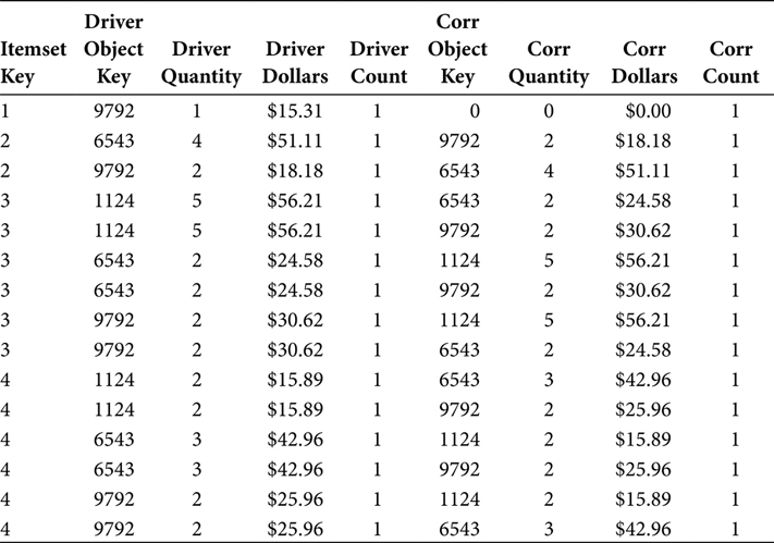
Step 2: Recursively Join the Market Basket Table and Load a Market Basket BI Table
The second step joins the Market Basket Table to itself by referencing the Market Basket Table twice. The first reference to the Market Basket Table has the alias A. The second reference to the Market Basket Table has the alias B. In the RDBMS platform this has the effect of operating on the same Market Basket Table as though it were two separate tables. Chapter 6 explained a database design that will optimize this recursive join.
Figure 7.2 shows this recursive join and load into the Market Basket BI Table as a single operation. A Market Basket ETL application may perform this operation in one step, or it may perform it as a two-step operation. The important aspects of the SQL in Figure 7.2 are the recursive join and the nonequality.
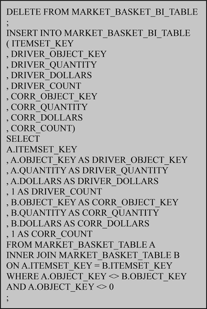
FIGURE 7.2
Load Market Basket BI Table.
The recursive join juxtaposes all the objects in an Itemset against all the other objects in an Itemset. This is the crux of the Market Basket Analysis application as it provides the first answer to the question in the Market Basket Scope Statement. The recursive join juxtaposes the Driver and Correlation Objects in a single row of data for the first time.
The inequality at the bottom of Figure 7.2 (A.OBJECT_KEY <> B.OBJECT_KEY) prevents an object in the Itemset from joining to itself. Without that inequality, all objects in an Itemset would have one row wherein that object is both the Driver Object and the Correlation Object. However, with that inequality in place, an object can be only the Driver Object or the Correlation Object, never both.
The other inequality at the bottom of Figure 7.2 (A.OBJECT_KEY <> 0) prevents the zero-filled row that was manufactured for the case of the Single Object Itemset from appearing as a Driver Object. Table 7.3 shows the effect of this inequality. The first two rows of Table 7.3 show the Single Object Itemset as it would be without the inequality. In one row, the Object_Key 15 is the Driver Object and Object_Key 0 is the Correlation Object. In the other row, the Object_Key 0 is the Driver Object and Object_Key 15 is the Correlation Object. The meaning of the zero-filled row for the Single Object Itemset is to indicate that nothing happened. When a customer purchases one item, what else did that customer purchase? Nothing. So, rather than allow a zero-filled row to be a Driver Object, the inequality excludes rows wherein the Driver_Object_Key = 0.
The Market Basket Table was a staging table. Reading the data from the Market Basket Table, the SQL in Figure 7.2 performs the recursive join, prevents objects from being both the Driver Object and the Correlation Object, and prevents the zero-filled object from being a Driver Object as it then loads the data into the Market Basket BI Table. The output of this SQL and the rows in the Market Basket BI Table are shown in Table 7.4.
The DRIVER_COUNT and CORR_COUNT output fields facilitate a count of the distinct objects in an Itemset. These two fields are manufactured in the SQL by the statements “1 AS DRIVER_COUNT” and “1 AS CORR_COUNT.” The manufacture of these fields could be delayed until the next step. However, understanding and validating the data in the Market Basket tables is confusing enough on its own. The analysts in a Market Basket Analysis effort are often better served by the presence of these COUNT fields in the Market Basket BI Table than by assuming their presence in the Market Basket BI View.
TABLE 7.3
Single Object Itemset
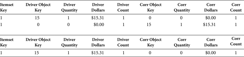
TABLE 7.4
Market Basket BI Table
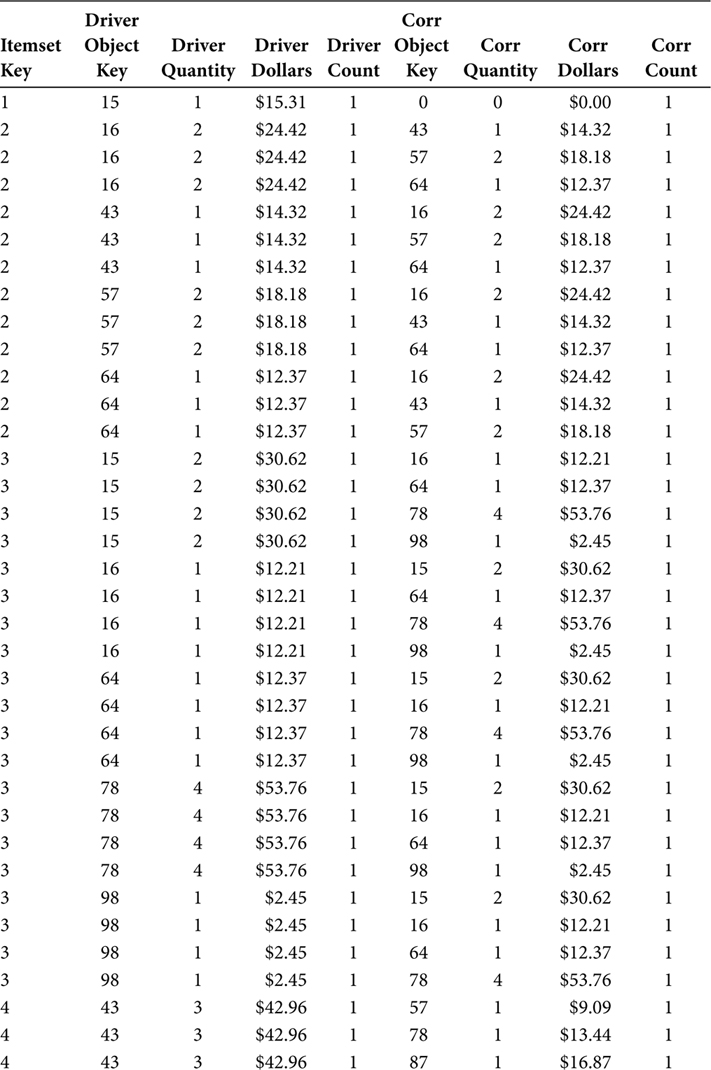
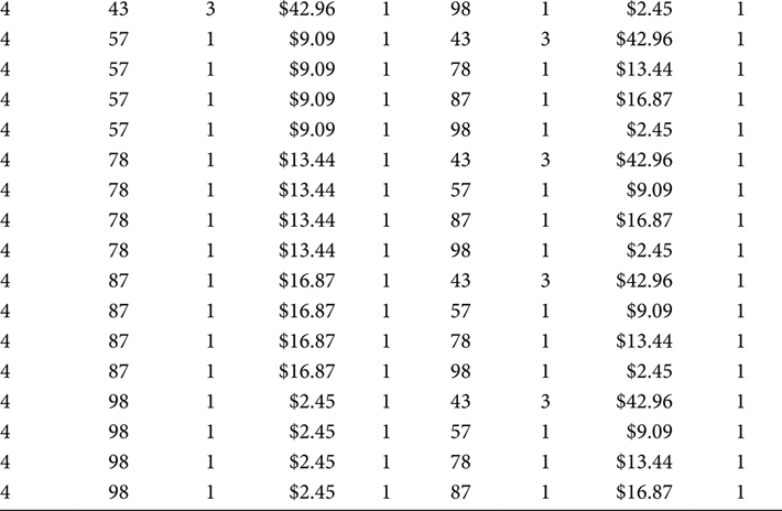
The Market Basket BI Table is the first table that may be customer-facing toward an analyst. As the Market Basket BI Table juxtaposes the Driver Object and Correlation Object with all the metric measurements included, it can be the terminus for an iteration of analysis.
Step 3: Arithmetic Juxtaposition of Driver Objects and Correlation Objects
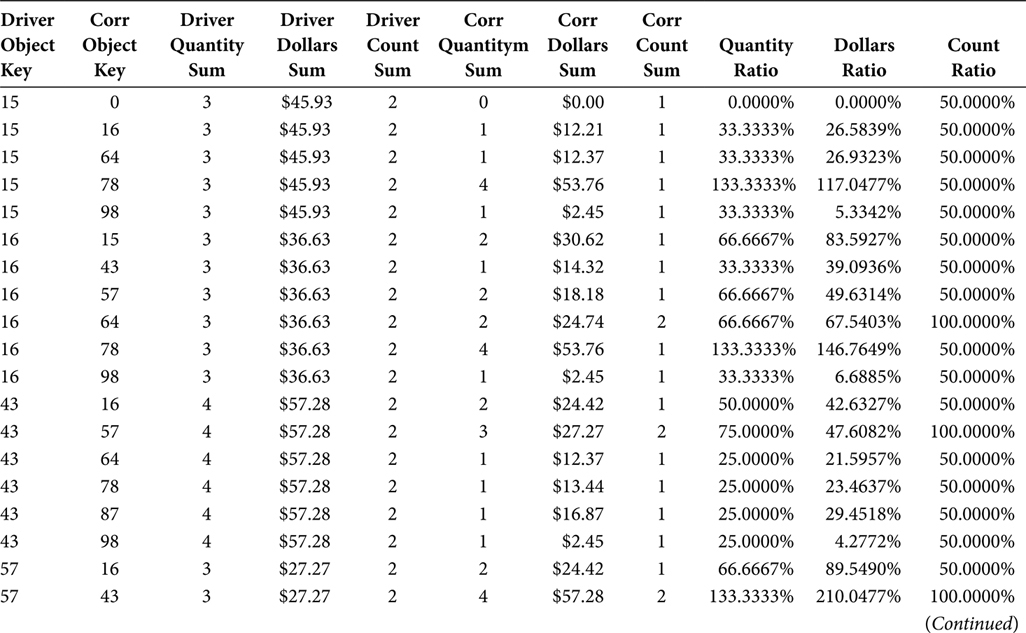
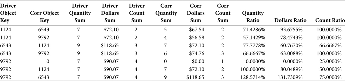
The Market Basket BI View, shown in Figure 7.3, arithmetically removes the Itemset from the juxtaposition of the Driver Object and Correlation Object. The additive metrics in the Market Basket Table (i.e., Quantity and Dollars) are both present in the Market Basket BI View as summations of the Quantity and Dollar fields. The Market Basket Analysis BI View also calculates ratios based on the summed additive metrics. The ratios provide a relative frame of reference that enhances the inferences that can be gleaned from the Market Basket Analysis.

FIGURE 7.3
Market Basket Analysis BI View.
The output from the Market Basket Analysis BI View, shown in Table 7.5, includes the additive and relative data columns. If a Market Basket Analysis effort is early in its life cycle, it will perform more of an analytics function than a reporting function. If that is the case, then the Market Basket Analysis BI View may persist as only a view. If, however, the Market Basket Analysis effort is in its maturity, then the stable and repeated Market Basket Reporting functions have begun. If that is the case, then the SQL in the Market Basket Analysis BI View should be performed as a final step in an ETL application that culminates in a Market Basket Analysis BI report. That would mean the Market Basket Analysis BI View is a table that can be referenced by the Market Basket Reporting application and the business analysts who receive reports from that application, which would mean the table created from the Market Basket Analysis BI View is the terminus of the Market Basket Analysis, rather than the Market Basket BI Table in Step 2.
TABLE 7.5
Market Basket Analysis BI View
Step 4: Load a Market Basket BI Table Using a Correlation Hierarchy
The Market Basket Analysis BI View is very powerful in that it provides cumulative and relative information about the correlations between objects in the Itemsets of an enterprise. That information, powerful as it may be, is limited in that it only considers objects that are hierarchical peers. An object is probably a member of hierarchical groupings (e.g., departments, regions, distribution channels). A successful Market Basket Analysis effort will soon lead to an analysis of the correlations between an object and hierarchies above that object. A retail clothing store might analyze the correlations between each individual shirt and the hierarchical group called “pants.” An automotive parts retailer might analyze the correlations between each individual brand of motor oil and the hierarchical group called “miscellaneous” (i.e., those little knickknacks at the front of the store). For that form of Market Basket Analysis, the objects must be juxtaposed with their hierarchical grouping.
To facilitate this discussion the hierarchical table in Table 7.6 will provide the hierarchies. The hierarchies in Table 7.6 can mean anything. The names of the hierarchies are not important. The presence and groupings of the hierarchies constitute the relevance of Table 7.6.
The Market Basket data already exists in its juxtaposed form in the Market Basket BI Table. This step will leverage the presence of the juxtaposed data in the Market Basket BI Table. The SQL in Figure 7.4 loads a new Market Basket table called MARKET_BASKET_BI_TABLE_CORR_HIERARCHY. This reflects an architectural decision to segregate separate sets of Market Basket data into separate tables, rather than by a type code in a single table. By the time a Market Basket Analysis effort reaches maturity, you’ll have quite a few efforts and even more tables present at any one time. So, a method for keeping them organized should be chosen earlier rather than later.
TABLE 7.6
Hierarchy Dimension
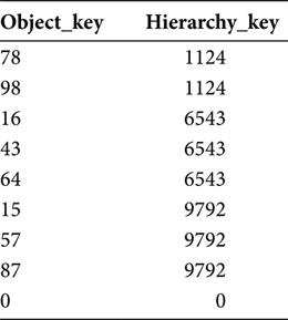
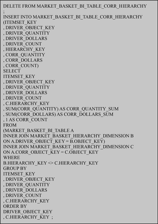
FIGURE 7.4
Load Market Basket BI Table with correlation hierarchy.
The SQL in Figure 7.4 performs three primary functions as it extracts data from the Market Basket BI Table and loads it into the MARKET_BASKET_BI_TABLE_CORR_HIERARCHY table. First, the “1 AS CORR_COUNT” statement resets the counter that will be used to count the number of occurrences of each hierarchical group within each Itemset. When combining objects into their hierarchical groups this counter is not additive. So, it is reset back to one, meaning the hierarchical group appeared once in an Itemset. This is true even if a hierarchical group was represented by two hundred objects. In the binary sense, a hierarchical was in, or not in, an Itemset.
The second primary function of the SQL in Figure 7.4 is that it joins the Driver Object to the hierarchy and then joins the Correlation Object to the hierarchy as a separate alias. The use of a separate alias for the hierarchy join causes the RDBMS platform to handle the two joins and join table independently of each other, even though they are the same tables.
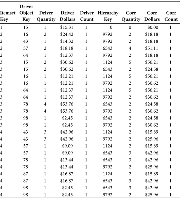
The third primary function of the SQL in Figure 7.4 is that it excludes those rows that join to the same hierarchical group for both the Driver Object and the Correlation Object. This has the effect of preventing a Driver Object from correlating to its own hierarchical group, which is conceptually the same as preventing an object from correlating with itself. The output of this is shown in Table 7.7.
The Market Basket Analysis BI View shown in Figure 7.5 is very similar to that in Figure 7.3. The difference is that the Correlation Object in Figure 7.5 has the name Hierarchy_Key, not CORR_OBJECT_KEY. Again, this reflects the need to organize the tables in a Market Basket Analysis application, by using column names that reflect the nature of the data in them. But, in general, the SQL in Figure 7.5 operates in a fashion similar to the SQL in Figure 7.3.
The output of the SQL in Figure 7.5 is shown in Table 7.8. The data in Table 7.8 can be presented in the form of a view or a physical table. The criteria for that decision are the same as the criteria for the decision to present the Market Basket Analysis BI View as a view or a physical table. A Market Basket Analysis effort that is still in the analysis, and not the reporting, phase would benefit from the use of a view and avoidance of the overhead of another table. A Market Basket Analysis effort that is in the reporting phase would benefit from the use of a physical table, which would be a datamart.
TABLE 7.7
Market Basket BI Table with Correlation Hierarchy
Step 5: Load a Market Basket BI Table Using a Driver Hierarchy
If a Market Basket Analysis effort can consider the correlations from objects leading to hierarchical groups, then that same Market Basket Analysis effort can also consider the correlations from hierarchical groups leading to objects. Using again the hierarchical groups in Table 7.6, the SQL in Figure 7.6 extracts data from the Market Basket BI Table and loads the MARKET_BASKET_BI_TABLE_DRIVER_HIERARCHY table.
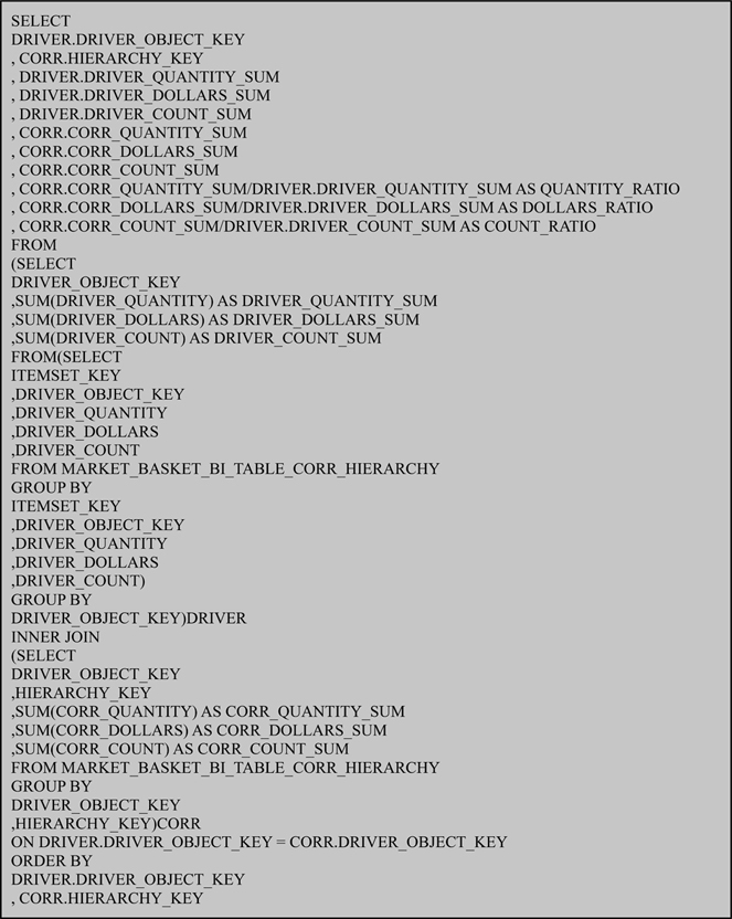
FIGURE 7.5
Market Basket Analysis BI View with correlation hierarchy.
The SQL in Figure 7.6 performs three primary functions as it extracts data from the Market Basket BI Table and loads it into the MARKET_BASKET_BI_TABLE_DRIVER_HIERARCHY table. First, the “1 AS DRIVER_COUNT” statement resets the counter that will be used to count the number of occurrences of each hierarchical group within each Itemset. When combining objects into their hierarchical groups this counter is not additive. So, it is reset back to one, meaning the hierarchical group appeared once in an Itemset. This is true even if a hierarchical group was represented by two hundred objects. In the binary sense, a hierarchical was in, or not in, an Itemset.
TABLE 7.8
Market Basket Analysis BI View with Correlation Hierarchy
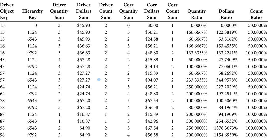
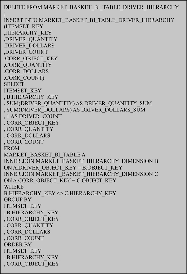
FIGURE 7.6
Load Market Basket BI Table with driver hierarchy.
The second primary function of the SQL in Figure 7.6 is that it joins the Driver Object to the hierarchy and then joins the Correlation Object to the hierarchy as a separate alias. The use of a separate alias for the hierarchy join causes the RDBMS platform to handle the two joins and join table independently of each other, even though they are the same tables.
TABLE 7.9
Market Basket BI Table with Driver Hierarchy
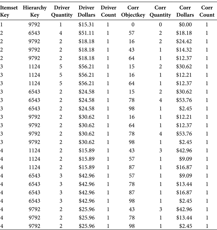
The third primary function of the SQL in Figure 7.6 is that it excludes those rows that join to the same hierarchical group for both the Driver Object and the Correlation Object. This has the effect of preventing a hierarchical group from correlating to its own objects, which is conceptually the same as preventing an object from correlating with itself. The output of this is shown in Table 7.9.
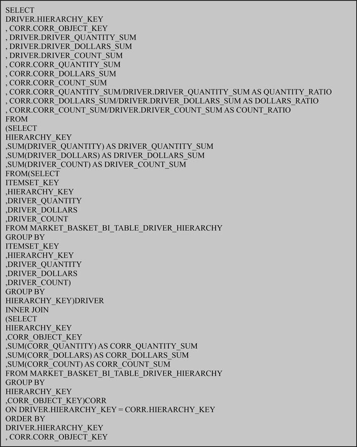
FIGURE 7.7
Market Basket Analysis BI View with driver hierarchy.
The Market Basket Analysis BI View shown in Figure 7.7 is very similar to that in Figure 7.3 and Figure 7.5. The difference is that the Driver Object in Figure 7.7 has the name Hierarchy_Key, not DRIVER_OBJECT_KEY. Again, this reflects the need to organize the tables in a Market Basket Analysis application, by using column names that reflect the nature of the data in them. But, in general, the SQL in Figure 7.7 operates in a fashion similar to the SQL in Figure 7.3 and Figure 7.5.
TABLE 7.10
Market Basket Analysis BI View with Driver Hierarchy
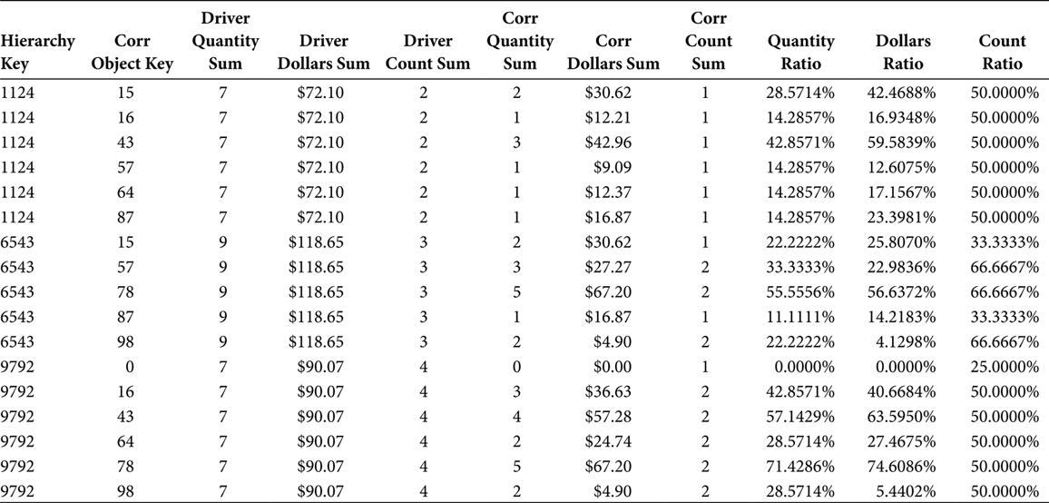
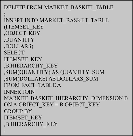
FIGURE 7.8
Load Market Basket Table with hierarchies.
The output of the SQL in Figure 7.7 is shown in Table 7.10. The data in Table 7.10 can be presented in the form of a view or a physical table for the same criteria as discussed previously.
Step 6: Load a Market Basket BI Table Using the same Hierarchy as Driver and correlation
If a Market Basket Analysis effort can consider the correlations from objects leading to hierarchical groups, and hierarchical groups leading to objects, then that same Market Basket Analysis effort can also consider the correlations from hierarchical groups leading to hierarchical groups. It was inevitable. Using again the hierarchical groups in Table 7.6, the SQL in Figure 7.8 extracts data from the original Fact table and loads the MARKET_BASKET_TABLE.
This method works because the Driver Object and Correlation Object are hierarchical peers. Contrary to the method of organizing data into separate tables, this method shows that Market Basket Analysis methods apply to all hierarchies of objects when the Driver and Correlation Objects are hierarchical peers. When they are peers, no additional SQL is required to avoid self-identifying correlations obscured by an object and its hierarchical group.
TABLE 7.11
Market Basket Table with Hierarchies
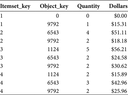
TABLE 7.12
Market Basket BI Table with Hierarchies
The Market Basket Table, loaded with objects represented by their hierarchical groups, is shown in Table 7.11. The number of rows decreases as the objects are abstracted up their hierarchies.
TABLE 7.13
Market Basket Analysis BI View with Hierarchies
The SQL in Figure 7.2 reads the Market Basket Table and loads the Market Basket BI Table. The output, shown in Table 7.12, is very similar to the output shown in Table 7.4. The difference is that the Object_Keys in Table 7.4 refer to objects while the Object_Keys in Table 7.12 refer to hierarchical groups of objects.
The output of the Market Basket BI View is shown in Table 7.13. This output is similar to the output shown in Table 7.5. The difference is that the Object_Keys in Table 7.5 refer to objects while the Object_Keys in Table 7.13 refer to hierarchical groups of objects.
Again, this shows that Market Basket Analysis methods apply to all hierarchies of objects when the Driver and Correlation Objects are hierarchical peers. These steps show how to perform Market Basket Analysis in three frames of reference:
Peer leading to Peer
Peer leading to Hierarchy
Hierarchy leading to Peer
These methods are important to a single Market Basket Analysis effort because all three will occur, yet they are not completely cumulative from one to the other. They also repeat at the point of Peer leading to Peer. The analytic phase of a Market Basket Analysis effort will follow this cycle up through the hierarchies of objects and then back down a different hierarchy of the same objects. So, a Market Basket ETL application must be able to traverse these levels of Market Basket Analysis through the hierarchical groupings of objects.