3	Improved Feature Vocabulary-Based Method for Image Categorization
	Frank Y. Shih and Alexander Sheppard

CONTENTS

3.1    Introduction

3.2    Feature Extraction and Description

3.3    Object Categorization

3.4    Improved Method Based on Random Sampling

3.4.1    K-Means Clustering and Nearest Neighbor Quantization

3.4.2    Nearest-Neighbor Classification as a Benchmark Method

3.4.3    Linear Soft-Margin SVMs

3.4.4    Categorization with Multi-Class SVMs

3.5    Experimental Results

3.6    Conclusions

References

3.1    INTRODUCTION

With the enormous and growing amounts of captured digital images, there has been tremendous interest in image categorization. Image categorization aims to label or classify images into one of the predefined categories. It attempts to retrieve all the images from the same category as a given query image. The attributes of similarity vary from system to system, which are mostly based on color, texture, and shape features.

Image categorization has a wide range of applications, including image search (Sivic and Zisserman, 2003), event detection (surveillance) (Li et al., 2005), process control (via robots or autonomous vehicles) (Loncomilla and Ruiz-del-Solar, 2005), and human–computer interaction (Nakajima et al., 2000). The use in such applications is primarily facilitated by the rising number of consumer devices employing digital image sensors, with mobile phones being a prominent example. A second factor is the continuing leaps in the computer-processing power, allowing for faster execution on image-processing algorithms.

Preceding our discussion, it is important to call attention to the distinction between object categorization and other similar but different tasks, such as object recognition, content-based image retrieval, and object detection. Object categorization entails associating some object present in an image with the correct label for that object. Object recognition can be said to identify one specific object instance, such as a particular red Honda Civic as opposed to a car. Content-based image retrieval deals mainly with low-level image features, not objects, and therefore may be quite imprecise. Object detection often focuses on a single visual category as opposed to many.

The bag-of-feature and feature vocabulary-based approaches have been presented for image categorization due to their simplicity and competitive performance. Some modified versions have been subsequently proposed, incorporating the methods such as adapted vocabularies, fast indexing, and Gaussian mixture models. In this chapter, we propose an improvement of replacing the Harris-affine detection method of Csurka et al. (2004) by a random sampling procedure together with an increased number of sample points (Shih and Sheppard, 2011).

The rest of the chapter is organized as follows. Section 3.2 describes feature extraction and description. Section 3.3 discusses object categorization. In Section 3.4, we present the improved method based on random sampling. Experimental results are provided in Section 3.5. Finally, we draw conclusions in Section 3.6.

3.2    FEATURE EXTRACTION AND DESCRIPTION

Feature extraction is the method for locating points of interest in an image that can be added to a database to be searched later in order to identify objects. Feature description is the method for describing the neighborhood of the located points in the database. In comparing various feature extraction and description methods, Moreels and Perona (2007) identified two leading candidates for real-time processing: one is the affine-invariant interest point detector by Mikolajczyk and Schmid (2002) and the other is Lowe’s scale-invariant features transform (2004).

The affine-invariant interest point detector is based on the Harris–Laplace detector (Mikolajczyk and Schmid, 2004; Lindeberg and Garding, 1994; Theodoridis and Koutroumbas, 2006), which is invariant only to scale change. This detector iteratively finds the scale-space extrema of the Laplacian-of-Gaussian (LoG) filter convolved with the image, identifies the maxima of the Harris corner measure taken at the selected scale, and repeats this process until two points are identical. This method is similar to Lowe’s Difference-of-Gaussian (DoG) detection method (Lowe, 2004) since DoG is a discrete approximation to LoG. The Harris–Laplace detector is briefly described as follows:

1.  Find the local extremum σ over scale of the LoG for the point x^(k); otherwise, reject the point. The investigated range of scales is limited to σ^(k+1) = t σ^(k) with t ∈ [0.7, 1.4].

2.  Detect the spatial location of a maximum of the Harris measure nearest to x^(k) for the selected σ^(k+1).

3.  Go to step 1 if σ^(k+1) ≠ σ^(k) or x^(k+1) ≠ x^(k).

However, this process fails for significant affine transformations due to the mapping of circular neighborhoods to elliptical neighborhoods in the affine transformed image. A modified detector intends to iteratively transform the neighborhood of a point and its affine-transformed version until these two neighborhoods can be related by a pure rotation matrix, which does not affect the LoG extremum since the magnitude of LoG is rotation-invariant. The formulae from scale-space theory are

$x^{\prime }{}_L=M_L^{-1/2}{x}_L, x^{\prime }{}_R=M_R^{-1/2}{x}_R, x^{\prime }{}_L=R{x}^{\prime }{}_R$

(3.1)

where M is the second moment matrix smoothed over the appropriate neighborhood and R is a pure rotation matrix. Provided that the necessary convergence criteria are satisfied, this implies that by iterating the application of the inverse second moment matrix over successive newly defined circular neighborhoods, it is possible to obtain a matrix U that will approach a fixed point, such that x = (μ^–1/2)^(k) x. Hence, μ must approach the identity matrix as k becomes large. Therefore, we have the following procedure:

1.  Initialize U⁽⁰⁾to the identity matrix.

2.  Normalize window W(x_w) = I(x) centered on U^(k–1)x_w^{(k– 1)} = x^{(k– 1)}.

3.  Select integration scale σ_I at point $x_{\text{w}}^{\left(k-1\right)}$.

4.  Select differentiation scale σ_D = sσ_I, where s maximizes λ_min(μ)/λ_max(μ) with s ∈ [0.5, 0.75] and μ = μ($x_{\text{w}}^{\left(k-1\right)}$), σ_I, σ_D).

5.  Detect spatial localization $x_{\text{w}}^{\left(k\right)}$ of a maximum of the Harris corner measure nearest to $x_{\text{w}}^{\left(k-1\right)}$ and compute the location of the interest point x^(k).

6.  Compute ${\text{μ}}_i^{\left(k\right)}\hspace{0.17em}=\hspace{0.17em}{\text{μ}}^{-1/2}\left(x_{\text{w}}^{\left(k\right)},{\text{σ}}_{\text{I}},{\text{σ}}_D\right)$.

7.  Concatenate transformation $U^{\left(k\right)}={\text{μ}}_i^{\left(k\right)}\cdot U^{\left(k-1\right)}$ and normalize U^(k) to λ_max(U^(k)) = 1.

8.  Go to step 2 if $1-\left({\text{λ}}_{\min }\left({\text{μ}}_i^{\left(k\right)}\right)/{\text{λ}}_{\max }\left({\text{μ}}_i^{\left(k\right)}\right)\right)\ge {\text{ε}}_C.$.

Once interest points have been identified, it is necessary to compute their descriptors. A standard method for this step is the scale-invariant feature transform (SIFT), which is pervasive in almost all the bags of keypoints categorization methods. The description involves first orienting the point neighborhood with respect to the image gradient, thus achieving rotation invariance to representation, and then representing the gradients around the point as a 4 × 4 array of histograms. Values are weighted using a Gaussian window with σ equal to one half the length of the histogram array, which ensures that changes in values fall off smoothly.

The descriptor is more robust than simply using image matching by correlation, which is highly sensitive to image changes that occur under 3D viewpoint change. To minimize abrupt changes in value, the descriptor uses trilinear interpolation to distribute the value of each gradient sample into adjacent bins. This avoids boundary effects between samples as they shift from one histogram to another. Also, to minimize disturbances from large nonlinear brightness changes near the image patch, all lengths are capped at a maximum of 0.2 (a value found by experimentation) and the vector is then renormalized. The main result is that each point is represented by a 4 × 4 × 8 = 128 dimensional feature vector.

3.3    OBJECT CATEGORIZATION

Csurka et al. (2004) proposed a simple, but effective, method for object categorization based on a bag of keypoints. Their method consists of the following steps:

1.  Assign feature descriptors to a set of predetermined clusters (a vocabulary) with a vector quantization algorithm.

2.  Construct a bag of keypoints, which counts the number of feature vectors assigned to each cluster.

3.  Apply a multi-class classifier, treat each bag of keypoints as the feature vector, and thus determine which category or categories to assign the image.

In order to generate the set of predetermined clusters, the simple method of k-means clustering is used based on assigning points to their closest cluster centers and then recomputing the cluster centers. It is described as follows:

1.  Choose initial estimates θ_j(0) arbitrarily for the θ_j cluster representatives, where j = 1, 2, …, m.

2.  While change still occurs, repeat:

a.  For i = 1, 2, …, N

i.	Determine the closest representative θj for x.
ii.	Set b(i) = j, where b maps member vectors to clusters.

b.  For j = 1, 2, …, m

Determine θ_j as the mean of the vectors x_i ∈ X with b(i) = j, where X is the complete set of vectors.

We can minimize the cost function:

$J\left(\text{θ},U\right)={\displaystyle \sum _{i=1}^N{\displaystyle \sum _{j=1}^m{u}_{ij}{\Vert x_i-{\text{θ}}_j\Vert }^2}}$

(3.2)

It means that the cost function recovers the clusters that are as compact as possible, as measured by the squared Euclidean distance. This can be represented in terms of vector quantizers Q, probability density function p(x), and vector quantizers R_j as

$\begin{array}{cc}Q\left(x\right)={\text{θ}}_j\text{iff d}\left(x,{\text{θ}}_j\right)\le \text{d}\left(x,{\text{θ}}_k\right),& k\text{=1, 2,}\dots .\text{, }m\text{, }k\ne j\end{array}$

(3.3)

${\displaystyle {\int }_{R_j}\text{d}\left(x,{\text{θ}}_j\right)p\left(x\right)\text{d}x=\underset{y}{\min }}{\displaystyle {\int }_{R_j}\text{d}\left(x,y\right)p\left(x\right)\text{d}x}$

(3.4)

The vector quantization method has a high impact on the time efficiency of constructing the histogram bins necessary for the bag-of-feature methods.

A disadvantage of the k-means algorithm is the lack of guarantee of convergence to a global minimum of the cost function, as opposed to a local minimum. Various strategies have been proposed to deal with this issue, such as initializing the cluster centers to the centers of a set of random partitions of the data, or using the optimization techniques such as genetic algorithms. However, these may be ineffective or may be costly in computation. Moreover, the bag-of-feature method is not primarily interested in the efficacy of clustering in terms of error, but rather in empirical discrimination during categorization. A second relevant feature of k-means is that the number of cluster centers is predetermined, which has a great effect on discriminative power up to a certain point. Beyond this point, results continue to improve to some extent, but it was found according to Csurka et al. (2004) that typically k = 1000 gives the best trade-off between computational speed and accuracy.

On completion of k-means, the set of clusters is formed into a histogram (the bag of keypoints) that counts the number of points assigned to each cluster. Each image can then be represented by such a histogram. A large database will contain many images, and hence many histograms will be generated. The histograms can be conceived as new feature vectors, which are fed into a classifier for training and testing. The classifiers may be the Naive Bayes Classifier or the support vector machine (SVM) with linear, quadratic, or cubic kernels.

In the proposed method, we use the random sampling method to produce improved categorization results over the keypoint-based detectors. We observe that using a large number of points in the initial clustering step tends to improve results. The scale-space extrema detected by the keypoint method are too few to ultimately compete with a larger random sample.

Nowak et al. (2006) identified four main implementation choices for bag-of-feature approaches, such as how to sample patches, which descriptor to use, how to quantify the resulting descriptor space distribution, and how to classify images based on the resulting global image descriptor. On the matter of the first implementation choice, random sampling on a pyramid in scale space is compared with Harris-affine and LoG detectors. Also, the size of the codebook (translating to the number of clusters if k-means were used) is examined. It is observed that as the codebook size increases, all approaches except random sampling begin to suffer from problems of dataset overfitting. Moreover, due to inherent limitations, Harris-affine and LoG cannot find sufficient points to compete with random sampling. Therefore, we propose an optimal categorization system using as large a keypoint sampling density as possible and a relatively large codebook size.

Notably, it is observed that although some methods of quantizing the data are helpful, the random construction of codebooks offers only relatively small disadvantages as compared with more sophisticated methods. In other words, the impact on bag-of-feature methods from the codebook construction algorithm (Csurka et al., 2004) is relatively slight as compared with sampling density, codebook size, and classifier design. The graphical representation of the variation of codebook construction algorithm is shown in Figure 3.1.

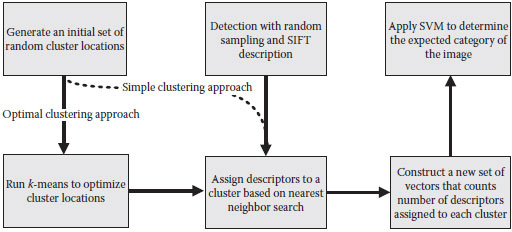
FIGURE 3.1 The graphical representation of the variation of codebook construction algorithm.

3.4    IMPROVED METHOD BASED ON RANDOM SAMPLING

To improve the method by Csurka et al. (2004), the optimized clustering approach should be taken as combined with the best possible detection method, random sampling, and a large number of sample points. In order to implement the description stage, the SIFT ++ program of Vedaldi (2005) was incorporated into the system. Vedaldi’s bag-of-feature program was used to generate random keypoints although the remainder of the program, which employs a hierarchical clustering strategy as opposed to k-means, was removed. For lucid comparisons, our program is run on the same Caltech 4 dataset in (Csurka et al., 2004). This generates up to 5000 random keypoints per image. Five image categories are used: car side views, car rear views, faces, airplanes, and motorbikes. Some images are shown in Figure 3.2. The number of images used is 450 per category, forming a total of 2250 images.

3.4.1    K-MEANS CLUSTERING AND NEAREST NEIGHBOR QUANTIZATION

For clustering and vector quantization, the SciPy library of algorithms and mathematical tools are employed in the Python programming language. The PyML is an interactive object-oriented framework for machine learning written in Python. Once loaded into SciPy, a relatively small subsample (5000 keypoints per category) of the entire dataset is used in simple k-means to generate a codebook of optimized cluster locations. The 1000-D feature vector representing each image is initialized to zero. Each keypoint vector is then compared with each of the optimized cluster locations to quantize it to an appropriate location in the codebook. For each image, the cluster location selected is then incremented in the 1000-D feature vector representing the entire image. From this process, a complete set of 1000-D histogram vectors is generated, each providing a unique representation of one image.

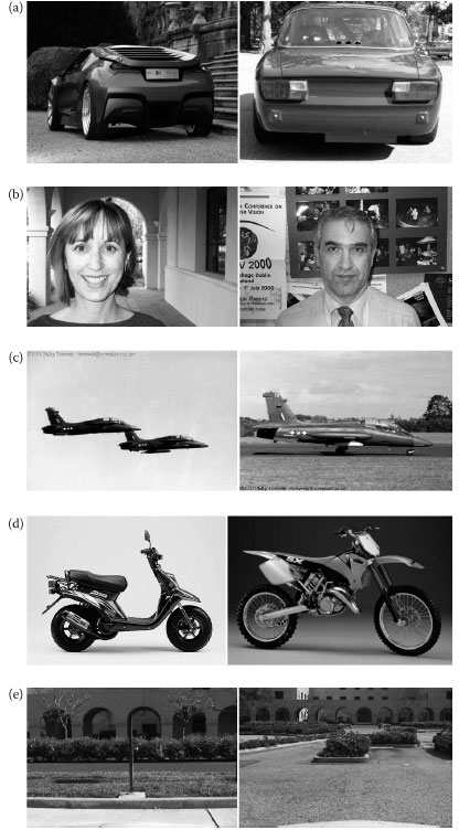
FIGURE 3.2 Image categories selected from the Caltech 4 database.

3.4.2    NEAREST-NEIGHBOR CLASSIFICATION AS A BENCHMARK METHOD

The classifier step is critical in the bag-of-feature method. Two basic approaches are employed: Bayesian classifier and SVM, with the former serving as benchmark for the latter. The Bayesian classifier is based on minimizing the probability of error using Bayesian statistical prediction. Applying this to the bag-of-feature method yields

$P\left(C_j|I_i\right)=P\left(C_j\right){\displaystyle \prod _{t=1}^{\left|V\right|}P{\left(v_t|C_j\right)}^{N\left(t,i\right)}}$

(3.5)

where C_j denotes the categories, I_i denotes images (corresponding to classes and vectors), v_t denotes the keypoint, and N(t, i) is the number of times that the cluster occurs in an image.

However, in order to vary the results, we use the k-nearest neighbor algorithm in place of Bayesian classification. This method is a nonparametric method classifying each point in the testing data according to the classes of the k closest vectors in the training data. Motivation comes from Bayesian theory: Given a small region R in the neighborhood of a test point x, the probability P of finding a training point in R, and N observations, we have K ≈ NP, where K is the number of training points in R. If the volume of R is small, the probability density of the data p(x) on R will be approximately constant, or P ≈ p(x)V. Removing P from the set of equations gives the density p(x) ≈ (K/NV). Applying the following Bayesian formula:

$p\text{(}{C}_k|x\text{)=}\frac{p\left(x|C_k\right)p\left(C_k\right)}{p\left(x\right)}$

(3.6)

with density for class k: p(x | C_k) = K_k/N_kV and the class prior probabilities: p(C_k) = N_k/N yields

$p\text{(}{C}_k|x\text{)}=\frac{K_k}{K}$

(3.7)

In other words, the class with the highest K_k value is optimal.

3.4.3    LINEAR SOFT-MARGIN SVMs

A sophisticated classifier is the SVM (Abe, 2005; Bishop, 2006; Cheng and Shih, 2007), a learning system that separates two classes of vectors with an optimal separating hyperplane. An important property of the SVM is that its hyperplane is one of maximal margins: the distance between vectors of each class is the largest that can exist given the dataset. There are several basic types of SVM, including the relatively simple linear maximal margin classifier, the linear soft margin classifier, and in the case where a nonlinear curve produces an optimal result; a nonlinear kernel function can be used to create a nonlinear classifier. In this chapter, we only consider the linear soft margin case because the linear maximal margin is too simple and using nonlinear kernels has been found to produce overfitting.

Given a set of training data x₁, x₂, …, x_k with x_i ∈ Rⁿ for i = 1, 2, …, k. The maximal margin hyperplane must be represented by the equation: w · x + b = 0, where w ∈ Rⁿ and b ∈ R. It is assumed to be possible to divide the training data into two classes, represented by a mapping to a y_i ∈ Rⁿ such that

$\{\begin{array}{cc}{w}^{\text{T}}{x}_i+b\ge 1& \text{for }{y}_i=1\\ w^{\text{T}}{x}_i+b<1& \text{for }{y}_i=-1\end{array}$

(3.8)

which is equivalent to

$y_i\left(w^T{x}_i+b\right)\ge 1\text{for }i\text{=1,}\dots \text{, }M$

(3.9)

Planes that satisfy this criterion are given by

$\begin{array}{cc}\left(w^{\text{T}}{x}_i+b\right)=c& \text{for }-\text{1}\text{<}c\text{<1}\end{array}$

(3.10)

Assuming that each plane with c = 1 and -1 includes at least one data point, the plane with c = 0 will provide maximal margin. It can be easily shown that the distance between any data point x and the optimal hyperplane is given by

$\frac{\left|D\left(x\right)\right|}{\left|w\right|}=\frac{\left|w^{\text{T}}x+b\right|}{\left|w\right|}$

(3.11)

Therefore, the maximal margin is simply 2/|w|. This is maximized if the function Q(w) = |w|²/2 is minimized with respect to the constraints given by the data. This can be reduced to an equivalent minimization problem:

$Q\left(w,b,\text{ξ}\right)\frac{1}{2}{\left|w\right|}^2+C{\displaystyle \sum _{i=1}^M{\text{ξ}}_i^p}$

(3.12)

which in turn is reduced to a quadratic programming problem except that C ≥ α_i is added as an additional constraint and p = 1 for present purposes. For the dataset, C is set to be 0.005.

3.4.4    CATEGORIZATION WITH MULTI-CLASS SVMs

There are several possible extensions of SVM to multi-class problems. Two most important extensions are one-against-all and pairwise coupling. The former is based on computing n decision functions, one for each class. If $D_i\left(x\right)\hspace{0.17em}=\hspace{0.17em}{w}_i^{T}x+b_i$ is the decision function between two classes i and j, $R_i\hspace{0.17em}=\hspace{0.17em}\left\{x|D_i\left(x\right)>0,i\hspace{0.17em}=\hspace{0.17em}n{\text{ and D}}_i\left(x\right)\le 0,\text{ i}\ne \text{n}\right\}$ are non-overlapping regions such that class n is favored above all others. On the other hand, for x ∉ R_i i = 1, 2, … n, we use membership functions defined based on the distance from the optimal separating hyperplanes D_j(x) = 0. In the case i = j, we have

$m_{ii}\left(x\right)=\{\begin{array}{cc}1& {\text{for D}}_i\left(x\right)\ge 1\\ {\text{D}}_i\left(x\right)& \text{otherwise}\end{array}$

(3.13)

and in the case i ≠ j, we have

$m_{ij}\left(x\right)=\{\begin{array}{cc}1& {\text{for D}}_j\left(x\right)\le -1\\ -{\text{D}}_j\left(x\right)& \text{otherwise}\end{array}$

(3.14)

A test vector x is assigned to the class: $\arg \underset{i=1,\dots ,n}{\min }{D}_i\left(x\right)$ provided that there is only one minimum. This scheme resolves the potential existence of unclassifiable regions.

3.5    EXPERIMENTAL RESULTS

In this section, the results of using the proposed method on the Caltech 4 dataset are presented. The images previously known to be in a particular category are inputted to the multi-class classifier. The classifier then uses the 1000 data attributes of the histogram vector to come up with its own classification. The classification is then compared with the known ground truth value to produce error measures. Four major runs are performed on 2250 images. Each of them uses seven values for keypoints per image in the interval of 5–5000. Description of the four major runs is presented in Table 3.1. Figure 3.3 illustrates the graphical comparison of the results.

Details for each run are described as follows. In all cases where the SVM classifier is used on histogram vectors, the parameter C is set to be 0.005 although the results appear almost identical for C = 1. For the k-NN classifier, k = 3. For building the vocabulary using k-means, 5000 keypoints per category are aggregated into a set of 25,000, from which the 1000 cluster centers are extracted. A random subset of feature vectors is also tried for a vocabulary in run 4. Finally, for high numbers of points allowed, the available number of SIFT keypoints begins to decline. In particular, for 1581 points the average actual number is decreased to 1272, and at 5000 it is only 2865.

TABLE 3.1
Description of Four Major Runs

	Classifier	Vocabulary	Detector
Run 1	SVM	k-means	Random
Run 2	SVM	k-means	SIFT
Run 3	k-NN	k-means	Random
Run 4	SVM	Random	Random

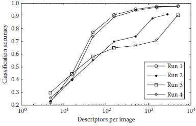
FIGURE 3.3 A graphical comparison of the results.

Results show that the SVM outperforms k-NN classification in the bag-of-feature methods. However, the most important result is that random keypoint locations conclusively outperform the SIFT detector even with the same number of keypoints. Thus, the new method is superior to the traditional methods. In particular, its accuracy on Caltech 4 reaches as high as 97.6%, which is 1.5% higher than the previous result (Csurka et al., 2004) and more than 6% higher in this implementation as compared with SIFT detectors at maximum accuracy. Table 3.2 shows the classification rate for each run and the number of keypoints used. All steps of the classification process can be implemented efficiently. The total time to classify all objects in Figure 3.3 is < 0.2 s on a 2 GHz Pentium 4 processor.

The performance of SIFT keypoints in this implementation is noticeably poor, with only 91.4% maximum accuracy. This may be due to the SIFT detector used as opposed to the newer Harris affine detector used. Another issue is that for high numbers of allowed points, SIFT cannot procure as many as a random sample. At 5000 points allowed, the actual mean number of SIFT keypoints found per image is only 2865. However, it appears that the large majority of the difference is due to the SIFT detector drawing an inherently poorer sample since the difference in accuracy between 1581 and 5000 keypoints is a mere 0.4% in Run 1.

TABLE 3.2
The Classification Rate for Each Run and the Number of Keypoints Used

The positive effect of using k-means to optimize the vocabulary appears to be small but consistent for large numbers of points used. Vocabulary composition has a significant effect on classification accuracy: for large numbers of points, a completely random vocabulary appears to drop the accuracy over using a random sample of keypoints, and performing k-means improves it by up to 0.2%.

Finally, confusion matrices are shown below for each run at maximum accuracy. Their graphical plot with SVM using k-means and 5000 random keypoints in the order of cars_brad, cars_brad_bg, motorbikes_side, faces, and airplanes_side in Run 1 is shown in Figure 3.4.

$\begin{array}{cc}\text{Run}\text{1}\text{:}& \text{Run}\text{2}\text{:}\\ \left[\begin{array}{ccccc}95.6& 0.4& 1.8& 0& 1.6\\ 0& 99.3& 0.4& 0& 0\\ 1.1& 0.2& 97.6& 0.2& 0.2\\ 0.7& 0& 0& 98.2& 0.7\\ 2.7& 0& 0.2& 1.6& 97.3\end{array}\right]& \left[\begin{array}{ccccc}89.8& 0.2& 0& 2.7& 5.6\\ 0.2& 95.3& 4.0& 0.2& 3.6\\ 0.4& 3.3& 95.3& 0& 2.0\\ 2.4& 0& 0& 91.1& 4.0\\ 7.1& 1.1& 0.2& 6.0& 84.9\end{array}\right]\end{array}$

$\begin{array}{cc}\text{Run}\text{3}\text{:}& \text{Run}\text{4}\text{:}\\ \left[\begin{array}{ccccc}93.6& 5.6& 4.0& 2.2& 14.7\\ 0& 92.2& 0& 0.4& 2.4\\ 4.9& 2.2& 95.8& 0.9& 6.2\\ 1.1& 0& 0& 96.0& 1.6\\ 0.4& 0& 0.2& 0.4& 74.9\end{array}\right]& \left[\begin{array}{ccccc}94.4& 0.4& 2.2& 0& 1.8\\ 0.2& 99.1& 0.2& 0& 0\\ 1.8& 0.2& 97.3& 0& 0\\ 0.7& 0& 0& 98.7& 0.9\\ 2.9& 0.2& 0.2& 1.3& 97.1\end{array}\right]\end{array}$

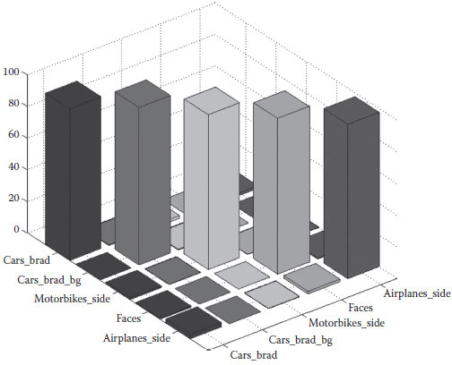
FIGURE 3.4 Graphical plot of the confusion matrix with SVM using k-means and 5000 random keypoints in Run 1.

3.6    CONCLUSIONS

The described new improvement is to replace the Harris-affine detection method by a random sampling procedure together with an increased number of sample points. We observe that using a large number of points in the initial clustering step tends to improve results. The scale-space extrema detected by the keypoint method are too few to ultimately compete with a larger random sample. Experimental results show that the classification of cluster histogram (bag of keypoints) vectors using random sampling and a large number of keypoints significantly outperforms the methods based on local features and the same number of keypoints. Mean classification accuracies exceed those of the latter methods by at least 6% in the proposed system, and exceed those using the k-NN classifier by at least 7%, giving an average of 97.6% accuracy on the Caltech 4 dataset. This value beats previously published results in (Csurka et al., 2004) by 1.5%.

REFERENCES

Abe, S., Support Vector Machines for Pattern Classification, Springer, New York, 2005.

Bishop, C., Pattern Recognition and Machine Learning, Springer, New York2006.

Cheng, S., and Shih, F.Y., An improved incremental training algorithm for support vector machines using active query, Pattern Recogn, 40(3), 964–971, 2007.

Csurka, G., Dance, C. R., Fan, L., Willamowski, J., and Bray, C., Visual categorization with bags of keypoints, Proc ECCV Intl Workshop on Statistical Learning in Computer Vision, pp. 1–24, 2004.

Li, Y., Atmosukarto, I., Kobashi, M., Yuen, J., and Shapiro, L. G., Object and event recognition for aerial surveillance, Proc SPIE Optics and Photonics in Global Homeland Security, 5781, Orlando, FL, pp. 139–149, may 2005.

Lindeberg, T., and Garding, J., Shape-adapted smoothing in estimation of 3-D shape cues from affine deformations of local 2-D brightness structure, Proc of European Conf on Computer Vision, Stockholm, Sweden, pp. 389–400, may 1994.

Loncomilla, P., and Ruiz-del-Solar, J., Improving SIFT-based object recognition for robot applications, Lect Notes Comput Sci, 3617, 1084–1092, 2005.

Lowe, D., Distinctive image features from scale-invariant keypoints, Intl J Comput Vis, 60(2), 91–110, 2004.

Mikolajczyk, K., and Schmid, C., An affine invariant interest point detector, Proc of European Conf on Computer Vision—Part I, Copenhagen, Denmark, pp. 128–142, May 2002.

Mikolajczyk, K., and Schmid, C., Scale and affine invariant interest point detectors, Intl J Comput Vis, 60(1), 63–86, 2004.

Moreels, P., and Perona, P., Evaluation of features detectors and descriptors based on 3D objects, Intl J Comput Vis, 73(3), 263–284, 2007.

Nakajima, C., Pontil, M., and Poggio, T., Object recognition and detection by a combination of support vector machine and rotation invariant phase only correlation, Proc Intl. Conf Pattern Recognition, vol. 4, Washington, DC, pp. 4787–4790, Sep 2000.

Nowak, E., Jurie, F., and Triggs, B., Sampling strategies for bag-of-features image classification, Proc of European Conf on Computer Vision, Graz, Austria, pp. 490–530, May 2006.

Shih, F. Y., and Sheppard, A., An improved feature vocabulary based method for image categorization, Pattern Recognit and Artificial Intelligence, 25(3) 415–429, 2011.

Sivic, J., and Zisserman, A., Video google: A text retrieval approach to object matching in videos, Proc Intl Conf on Computer Vision, vol. 2, Nice, France. pp. 1470–1477, Oct 2003.

Theodoridis, S., and Koutroumbas, K., Pattern Recognition, Academic Press, Orlando, FL, 2006.

Vedaldi, A., SIFT++: A lightweight C++ implementation of SIFT 2005.http://vision.ucla.edu/~vedaldi/code/siftpp/siftpp.html.