6	Pseudo-Random Pixel Rearrangement Algorithm Based on Gaussian Integers for Image Watermarking
	Aleksey Koval, Frank Y. Shih and Boris S. Verkhovsky

CONTENTS

6.1    Introduction

6.2    Overview to Gaussian Integers

6.3    Pixel Rearrangement Algorithm

6.4    Proof of Algorithm Validity

6.5    Cryptoimmunity of the Rearrangement Algorithm

6.6    Comparison to Arnold’s Cat Map Chaos Transformation

6.7    An Example in Image Watermarking

6.8    Conclusions

References

6.1    INTRODUCTION

Steganography is a process of hiding information in a medium in such a manner that no one except for the anticipated recipient knows of its existence (Shih, 2008). The history of steganography can be traced back to around 440 B.C.E., where the Greek historian Herodotus described in his writings about two events: one used wax to cover secret messages, and the other used shaved heads. With the explosion of Internet as a carrier for various digital media, many new directions of this state of the art emerged.

A notable application of steganography is watermarking of digital images, which is a useful tool for identifying the source, creator, owner, distributor, or authorized consumer of a document or an image. It has become very easy nowadays to copy or distribute digital images (whether copyrighted or not). A watermark is a pattern of bits inserted into a digital media for copyright protection (Berghel and O’Gorman, 1996). There are two kinds of watermarks: visible and hidden. A good visiblewatermark must be difficult for an unauthorized person to remove and can resist falsification. Since it is relatively easy to embed a pattern or a logo into a host image, the authorized person must make sure that the visible watermark was indeed the one inserted by the author. In contrast, a hidden watermark is embedded into a host image by some sophisticated algorithm and is invisible to the naked eye. It could, however, be extracted by a computer.

There are many innovating watermarking algorithms and many more get published everyday (such as Al-Qaheri et al., 2010; Huang et al., 2010; Lin and Shiu, 2010; Yamamoto and Iwakiri, 2010). In many image watermarking algorithms, for example (Dawei et al., 2004; Wu and Shih, 2007; Yantao et al., 2008; Ye, 2010), it is required to rearrange the pixels as a part of watermarking process. Randomness is desired during this step. Modular arithmetic and, specifically, the integer exponentiation modulo prime numbers are widely used in modern cryptographic algorithms. One important property of integer exponentiation modulo prime is that it generates a sequence of integers that looks very much like a sequence of random numbers. This is a property that is desirable for pixel rearrangement algorithms. In this chapter, the rearrangement step of watermarking algorithms is revisited and a different universal method for doing it is described. It is easy to replace the rearrangement step in Dawei et al. (2004), Wu and Shih (2007), Yantao et al. (2008), and Ye (2010). Moreover, this method can be used with most image watermarking algorithms to enhance them.

One can look at Gaussian integers as an extension of real integers into two dimensions. They exhibit similar properties as regular integers but have some notable differences that could be exploited in various fields such as cryptography (El-Kassar et al., 2001, 2005; Elkamchouchi et al., 2002; Verkhovsky and Koval, 2008). One important difference is that they have a larger order for the same prime size, which provides the increased security.

Wu and Shih (2007) and Yantao et al. (2008) Arnold’s cat map (Arnold and Avez, 1968) was used to rearrange pixels for improving the performance of watermarking techniques. Here a replacement is described, namely, a novel pixel rearrangement algorithm based on Gaussian integers, to rearrange pixels in an image (Koval et al., 2010). It is demonstrated that the new algorithm is superior to Arnold’s cat map in both time complexity and security. This technique is not a watermarking algorithm by itself but rather a universal enhancement to any existing watermarking algorithms. The technique tends to increase robustness to noise by uniformly distributing noise throughout the image. The increase in robustness depends on the watermarking algorithm enhanced by the technique.

6.2    OVERVIEW TO GAUSSIAN INTEGERS

A Gaussian integer is a complex number: Z[i] = {a + bi : a, b ∈ ℤ}, where both a and b are integers. Gaussian integers, with ordinary addition and multiplication of complex numbers, form an integral domain. The norm of a Gaussian integer is a natural number, defined as |a + bi| = a² + b².

The prime elements of Z[i] are also known as Gaussian primes, and can be divided into two subgroups. One subgroup consists of primes P = (p, 0), where p is a realprime and (p mod 4) = 3, referred to as Blum primes. The second subgroup consists of primes P = (a, b), where |P| is a real prime and |P| mod 4 = 1 (real non-Blum prime), referred to as non-Blum Gaussian primes.

There is one-to-one relationship between groups modulo real non-Blum primes and non-Blum Gaussian primes. Owing to this fact, the algorithms based on such Gaussian integers do not offer any advantages over real integers. Hence, a subset of Z[i]: real primes p:(p mod 4) = 3 or Blum primes should be considered. This allows the following definition of modulo (mod) operation for Gaussian primes to be

$A\text{mod }p=\left(a\mathrm{mod}p\right)+\left(b\mathrm{mod}p\right)i.$

(6.1)

In this chapter, Gaussian integers are denoted with capital letters and real integers with lower case letters. Also, vector notation for Gaussian integers is used (i.e., G = (a, b) is equivalent to G = a + bi).

The order for Gaussian integers is defined in the same way as for real integers. k is called an order of a Gaussian integer H if H^k = (1.0) (mod p). This is equivalent to stating that

$\text{ord}\left(H\right)\mathrm{mod}p=k.$

(6.2)

The ideas in Karatsuba and Ofman (1962) could be applied to speed up multiplication of Gaussian integers. It takes three multiplications to multiply two different Gaussian integers. Below is the algorithm inspired by (Karatsuba and Ofman, 1962).

Algorithm 1:    Gaussian Integer Multiplication

Given: Gaussian integers (a,b) and (c,d).

Output: Gaussian integer (x,y) = (a,b)(c,d).

$\begin{array}{ccc}{v}_1:=\left(a+b\right)\left(c+d\right);& v_2:=ac;& v_3:=bd\end{array};$

(6.3)

$\begin{array}{cc}x=v_2-v_3;& y=v_1-v_2-v_3;\end{array}$

(6.4)

It takes two multiplications to square a Gaussian integer:

${\left(a,b\right)}^2=\left(\left(a+b\right)\left(a-b\right),ab+ab\right).$

(6.5)

For the main algorithm described in this chapter, the exponentiation of Gaussian integers modulo prime has to be performed. To do this, any one of the many published real integer exponentiation algorithms that have multiplication and square modulo prime as the basic step could be used. The only thing required to do is to replace real integers with Gaussian integers and use Algorithm 1 for multiplication and Equation 6.5 for squaring. As an example, the widely used left-to-right binary exponentiation algorithm (a form of Square-and-Multiply exponentiation algorithm) described in Menezes et al. (1997, Section 14.6) will be adopted.

Algorithm 2:  Left-to-Right Binary Exponentiation Algorithm for Gaussian Integer

Given: Gaussian integer G = (a, b), prime p, exponent e = (e_t e_t-1 … e₁ e₀)₂

Output: Gaussian integer A = G^e mod p

For squaring, on line 3 of Algorithm 2, one can use Equation 6.5 and for multiplication operation Algorithm 1 could be used. There are as many iterations of the main loop as there are bits in the exponent e. One squaring operation is performed for each iteration. Additionally, one multiplication is performed if the current e_i bit is 1 Assuming that e is random, the number of 1’s equals to the number of 0’s in e on average. Thus, the average number of integer multiplications in Algorithm 2 is

$3.5\left[{\log }_2\left(e\right)\right].$

(6.6)

The example below demonstrates the steps of Algorithm 2.

Example 1: Illustration of Algorithm 2

Suppose (1,2)³⁵⁷ mod 23 has to be computed. First note that e = 357₁₀ = 101100101₂. Set A: = (1,0) (line 1 of the Algorithm 2). After this, iterate through the bits of e = 101100101₂:

1.  i=8, e₈=1. Computing A=(1, 0)²mod 23=(1 , 0). Since e₈ =1, compute A=AG mod p=(1 , 0)(1 , 2) mod 23=(1 , 2).

2.  i=7, e₇=0. Computing A=(1, 2)² mod 23=(20, 4).

3.  i=6, e₆=1. Computing A=(20, 4)² mod 23=(16 , 22). Since e₆=1, compute A=AG mod p=(16, 22)(1, 2) mod 23=(18 , 8).

4.  i=5, e₅=1. Computing A=(18 , 8)² mod 23=(7 , 12). Since e₅=1, compute A=AG mod p=(7 , 12)(1 , 2)mod 23=(6 , 3).

5.  i=4, e₄=0. Computing A=(6 , 3)² mod 23=(4 , 13).

6.  i=3, e₃=0. Computing A=(4 , 13)² mod 23=(8 , 12).

7.  i=2, e₂=2, Computing A=(8 , 12)² mod 23=(12 , 8).Since e₂=1, compute A=AG mod p=(12 , 8)(1 , 2) i=5, mod 23=(19 , 9).

8.  i=1, e₁=0. Computing A=(19 , 9)² mod 23=(4 , 20).

9.  i=0, e₀=1. Computing A=(4 , 20)² mod 23=(7 , 22). Since e₀=1, compute A=AG mod p=(7 , 22)(1 , 2) mod 23=(9 , 13).

Therefore, (1,2)³⁵⁷mod 23 = (9,13)

For the main algorithm described in this chapter, it is necessary to find a special Gaussian integer called a generator, as defined below.

Definition 1 Gaussian Integer Generator

A Gaussian integer G is a generator for a Blum Gaussian prime p iff ord(G) = p² – 1 (mod p).

Generators are easy to find. To find a generator for the Gaussian integer group modulo prime p, the following algorithm is sufficient (improvement is possible for certain cases (Verkhovsky and Sadik, 2009)):

Algorithm 3:    A Simple Algorithm for Finding Gaussian Integer Generators

1.  Factor p² – 1:

$p^2-1={\left(f_1\right)}^{e_1}{\left(f_2\right)}^{e_2}\cdots {\left(f_k\right)}^{e_k}.$

(6.7)

2.  Select a Gaussian integer G = (a, b) such that a ≠ 0, b ≠ 0, and a² ≠ b²(mod p).

3.  For each factor f_i of p² – 1, compute

$B_i=G^{\raisebox{1ex}{$\left(p^2-1\right)$}\!\left/ \!\raisebox{-1ex}{$fi$}\right.}\mathrm{mod}p.$

(6.8)

If any of B_i = (1,0) mod p, then G is not a generator and go to Step 2. Otherwise, G is a generator. The example below demonstrates the steps of Algorithm 3.

Example 2: Illustration of Algorithm 3 (Finding of a Gaussian Generator)

Suppose a Gaussian generator for the prime p = 23 has to be found. At first, factor p² – 1:

$p^2-1={23}^2-1=528=2^4\cdot 3\cdot 11.$

(6.9)

After that, try G = (1,2). To see if G is a generator, compute:

${\left(1,2\right)}^{528/2}\mathrm{mod}23=\left(22,0\right).$

(6.10)

Since (22,0) is not (1,0), try the next factor of 528: integer 11.

$\text{i}{\left(1,2\right)}^{528/2}\mathrm{mod}23=\left(2,0\right).$

(6.11)

Since (2,0) is not (1,0), we obtain that (1,2) is a generator.

6.3    PIXEL REARRANGEMENT ALGORITHM

Algorithm 4:    Pixel Rearrangement Based on Gaussian Integers

Given: Image I = (x,y) of size m × n;

Output: Image I′ = (x′, y′) of size m × n;

1.  Generate a prime p > max(m, n)and p mod 4=3.

2.  Find a Gaussian integer generator G =(a , b)mod p using Algorithm 3.

3.  Generate a random number s, such that 0 > s > p²–1.

4.  

$S=\left(s_x,s_y\right):=G^s\mathrm{mod}p$

(6.12)

5.  while (s_x≤m or S_y≤n)

6.  S:=SG mod p

7.  end-while

8.  C=(c₁ , C₂) :=S

9.  for i=1 to m

10.   for j=1 to n

11.  

$I^{\prime }\left\{c_1,c_2\right\}:=I\left\{i,j\right\}$

(6.13)

12.  

$C:=CG\mathrm{mod}p$

(6.14)

13.    while c₁>m or c₂ > m

14.  

$C:=CG\mathrm{mod}p$

(6.15)

15.    end-while

16.   end-for

17.  end-for

Note that the last value of C = (c_l, c₂) needs to be saved in order to rearrange back the pixels. Without the value of C, pixels could be rearranged back; however, it would require additional computation.

Algorithm 5:    Reverse of Algorithm 4

1.  

$C_r:=C$

(6.16)

2.  for i=m downto 1

3.   for j=n downto 1

4.  

$I\left\{i,j\right\}:=I^{\prime }\left\{c_1,c_2\right\}$

(6.17)

5.  

$C_r:=C_r{G}^{-1}\mathrm{mod}p$

(6.18)

6.    while (c₁ > m or c₂> m)

7.  

$C_r:=C_r{G}^{-1}\mathrm{mod}p$

(6.19)

8.    end-while

9.   end-for

10.  end-for

The time complexity of Algorithms 4 and 5 can be defined in terms of p. The most computationally expensive operations of the algorithm are Equations 6.12, 6.14, and 6.18. Suppose that u is the time spent to multiply two integers of size p. Assuming that the Square-and-Multiply algorithm is used for exponentiation and Algorithm 1 is used to multiply two Gaussian integers, the time complexity of Equation 6.12 is approximately:

$3.5u{\log }_2\left(p^2-1\right)\simeq 7u{\log }_{2}p.$

(6.20)

Because the order of Gaussian integers is p² – 1, in Step 4 of Algorithm 4, p² – 1 multiplications are performed. Therefore, the number of multiplications required is

$\text{O}\left(3u\left(p^2-1\right)\right)=\text{O}\left(3u{p}^2\right).$

(6.21)

The total time complexity of Algorithm 4 is

$\text{O}\left(3u\left(p^2-1\right)+7u{\log }_{2}p\right)=\text{O}\left(u{p}^2\right).$

(6.22)

The complexity of integer multiplication u depends on the size of p. For small p, the most efficient algorithm is the naive multiplication with time complexity of O(l²), where l = log₂p is the size of p in bits. For a larger p, the multiplication algorithm in Karatsuba and Ofman (1962) is faster than the naive method. The time complexity of Karatsuba multiplication is O(3l^1.585). For an even larger p, Toom-Cook (or Toom-3) algorithm is more efficient with a time complexity of O(n^1.465) (Knuth, 1998). The thresholds for the size of p vary widely with implementation details. However, it is reasonable to assume that most images would not be sufficiently large for Toom-Cook or Karatsuba multiplication. Therefore, it can be assumed that the naive multiplication method can be used and Equation 6.22 becomes

$\text{O}\left(u{p}^2\right)=O\left[{\left(p{\log }_{2}p\right)}^2\right].$

(6.23)

which is the time complexity of Algorithm 4.

To minimize the time complexity, it is reasonable to select p close to max(m, n). If p is selected in such a way, then the time complexity in terms of image size is

$\text{O}\left\{{\left[\max \left(m,n\right){\text{log}}_2\left(\max \left(m,n\right)\right)\right]}^2\right\}.$

(6.24)

The rearrangement algorithm described above is universal and can be used for many purposes. It can be applied for image watermarking as follows.

Algorithm 6:    Watermarking with Pixel Rearrangement Based on Gaussian Integers

1.  Rearrange the image using Algorithm 4.

2.  Apply the desired watermarking technique to the resulting rearranged image from Step 1.

3.  Apply Algorithm 5 to the resulting image from Step 2.

Algorithm 7:    Extraction of the Watermark Applied with Algorithm 4

1.  Rearrange the image using Algorithm 4.

2.  Extract the watermark using the watermarking extraction technique in Algorithm 5.

Note that in Algorithm 5, depending on the watermarking technique, it may be possible to extract watermark and perform rearrangement on the watermark rather than on the image.

6.4    PROOF OF ALGORITHM VALIDITY

The validity of the algorithms arises from the properties of the Gaussian integer group. In this section, these properties are going to be described and proved. For any two complex numbers A and B, it is true that |AB| = |A||B|. Gaussian integer is a special kind of complex number, so it is true for Gaussian integers also. When a Gaussian integer C is multiplied by itself modulo p, in turn, the norm of C mod p gets multiplied by itself also. This means that |C|mod p (i = 1,2,…) will cycle with a period of ord(|C|)mod p, as illustrated in Tables 6.1 and 6.2.

In addition, C^ord(|C|) is a Gaussian integer with norm equal to 1 mod p. In fact, the Gaussian integers U: |U| = 1 mod p form a cyclic subgroup with an order (p + 1). This subgroup will be referred to as a Norm 1 subgroup. Moreover, the order of any Gaussian integer C is a product of ord(|C|) and ord(|U|), where U = C^ord(|C|) mod p. From this, the algorithms for finding Gaussian generators to use for discrete logarithm-based cryptography are derived.

Lemma 1

If C is a complex number and p is a prime, then |Cⁿ| = |C|ⁿ mod p.

Proof:

For any complex number, it is true that |Cⁿ| = |C|ⁿ; therefore, |Cⁿ| = |C|ⁿ mod p.

Q.E.D.

Lemma 2

If C is a Gaussian integer and p is a Blum prime, then

•  ord(C)mod p is divisible by ord(|C|)mod p

•  if C^ord(|C|) = U mod p, then |U| = 1mod p

•  if U = C^ord(|C|)mod p, then ord(C)mod p is divisible by ord(U)mod p

Proof:

Suppose that ord(C)mod p is not divisible by ord(|C|)mod p. This means that |C^ord(C)| mod p is not equal to 1, but C^ord(C) = (1,0). This is a contradiction. |U| must equal to 1 mod p because |Cⁿ| = |Cⁿ| mod p and, in this case, n = ord(|C|). If ord(C) mod p is not divisible by ord(U), then C^ord(C) would not equal to (1, 0), so ord(C) must be divisible by ord(U).

TABLE 6.1
Repeating Norm Examples for Prime p = 7

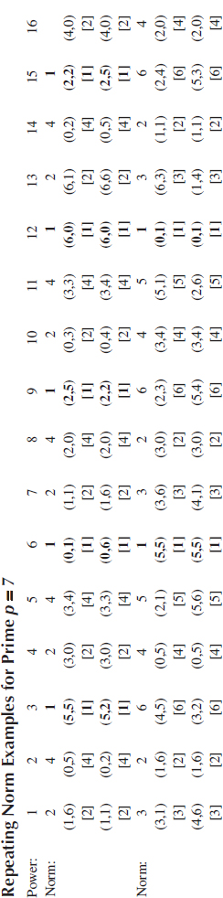
Note: The cases of Norm = 1 are in bold face.

TABLE 6.2
Repeating Norm Examples for Prime p = 7

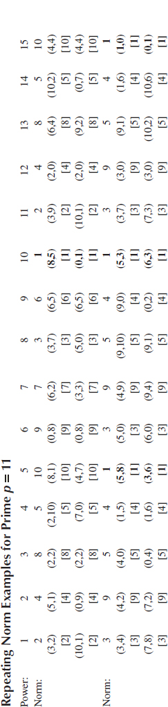
Note: The cases of Norm = 1 are in bold face.

Lemma 3

If U is a Gaussian Integer, p is a Blum prime, and |U| = 1 mod p, then

1.  The maximum order of U is (p + 1), and

2.  ord(U) mod p must divide (p + 1).

Proof:

1.  Any Gaussian integer A taken to the power (p + 1) mod p is in the form of (c, 0).

In this case, U^{p + 1} mod p could be one of either (1,0) or (–1,0) because |U| = 1 mod p. Since p + 1 is divisible by 4 for all Blum primes, U^(p+1)/4 is a Gaussian integer of norm 1 and is a root of degree of U^p+1. For (–1,0), all roots of degree 4 have a norm equal to –1 mod p. This means that U^{(p + 1)} must equal to (1, 0) mod p.

2.  If p1 + 1 is not divisible by ord(U), then U^(p+1) would not be equal to (1,0), so p + 1 must be divisible by ord(U).

Q.E.D.

Lemma 4

If C is a Gaussian integer and p is a Blum prime, then ord(C) = ord(|C|)ord(U) mod p, where |Cⁿ| = |C|ⁿ mod p.

Proof:

ord(C) must be divisible by ord(|C|) and ord(U), so ord(C) = n^*ord(|C|)ord(U), where n is an integer. In addition, C^ord(|c|)ord^(U) = U^ord(U) = (1, 0). Consequently, n must be equal to 1.

6.5    CRYPTOIMMUNITY OF THE REARRANGEMENT ALGORITHM

From the properties of the Gaussian integer group, it could be estimated how hard it is for an adversary to obtain the original image from the rearranged one. The less an adversary knows about the algorithm and parameters, the harder it is to determine the original arrangement. It is reasonable to look at the following three cases:

Case 1. The adversary knows nothing about the rearrangement algorithm used, but one suspects that some kind of algorithm has been used. In this case, it is extremelyhard for the adversary to figure out the original arrangement because there are too many possibilities. That is, there are n! possible permutations, where n is the number of pixels in the image.

Case 2. The adversary knows that Algorithm 4 was used, but one does not know the parameters such as prime p, generator G, or private key s. In this case, the number of possible permutations for an image I of size m × n is

$\left(p^2-1\right)\left[\text{φ}\left(p^2-1\right)\right].$

(6.25)

where φ is Euler’s totient function (Abramowitz and Stegun, 1964).

Equation 6.25 does not include the complexity of guessing p. The reason for this is that it is too computationally expensive to use a large p (refer to Equation 6.23). For efficiency, p should be close to the image size. The prime p in Equation 6.25 can be selected in such a way that φ(p − 1) is maximized. To do this, a prime with large prime divisors of p + 1 and p – 1 could be selected. For example,

$p+1=s_1{q}_1$

(6.26)

and

$p-1=s_2{q}_2,$

(6.27)

where s₁ and s₂ are small integers, and q₁ and q₂are primes close to p in size. In this case,

$\text{φ}\left(p^2-1\right)=\text{φ}\left(\left(p-1\right)\left(p+1\right)\right)=\text{φ}\left(s_1{s}_2\right)\left(q_1-1\right)\left(q_2-1\right)$

(6.28)

and

$\text{o}\left(\text{φ}\left(p^2-1\right)\right)=\text{ o}\left(\left(q_1-1\right)\left(q_2-1\right)\right)=\text{ o}\left(q_1{q}_2\right)=\text{ o}\left(p^2\right).$

(6.29)

Consequently, the approximate computational complexity is

$\text{o}\left(\left(p^2-1\right)\left[\text{φ}\left(p^2-1\right)\right]\right)=\text{ o}\left(p^4\right)=\text{ o}\left(\max {\left(m,n\right)}^4\right).$

(6.30)

Case 3. The adversary knows Algorithm 4 used, prime p, and a generator G. In this case, the number of possible permutations is limited to

$p^2-1.$

(6.31)

While it may be unreasonable to assume that the adversary would not know Algorithm 4, there is no reason to make a prime p and a generator G known. Therefore, case 2 may be the most reasonable security estimate.

If increased protection is desired, Algorithm 4 could be applied several times on the same image. Suppose that Algorithm 4 was applied t times on image I of size m × n. In this case, the number of possible permutations is

$\text{o}\left(\max {\left(m,n\right)}^{4t}\right),$

(6.32)

while the time to compute the rearranged image would still be reasonable and be on the same order in terms of image size:

$\text{O}\left\{t{\left[\max \left(m,n\right){\log }_2\max \left(m,n\right)\right]}^2\right\}=\text{ O}\left\{{\left[\max \left(m,n\right){\log }_2\max \left(m,n\right)\right]}^2\right\}.$

(6.33)

Therefore, one can achieve the desired level of security by increasing the time it takes to rearrange the image somewhat. Multiple rearrangements could provide a desirable and practical trade-off.

6.6    COMPARISON TO ARNOLD’S CAT MAP CHAOS TRANSFORMATION

The Arnold’s cat map transformation variation used in Wu and Shih (2007) is defined as

$\left[\begin{array}{c}{x}^{\prime }\\ y^{\prime }\end{array}\right]=\left[\begin{array}{cc}1& 1\\ l& l+1\end{array}\right]\left[\begin{array}{c}x\\ y\end{array}\right]\mathrm{mod}N,$

(6.34)

where N is the width of the square image. The possible values of l in Equation 6.34 are l: 1 < l < N − 2. Therefore, the number of the transformations required is O(N). It is reasonable to assume that N is small enough to call for naive multiplication algorithms. Thus, the multiplication time complexity is

$\text{O}\left({\log }_2^{2}N\right),$

(6.35)

which has to be performed for every pixel (i.e., N² times). Therefore, the time complexity of Arnold’s Cat Map is

$\text{O}\left(N^3{\log }_2^{2}N\right).$

(6.36)

Equation 6.26 should be compared with Equation 6.24, assuming N ≃ max(m, n). It is obvious that the computational complexity of Algorithm 4 described by Equation 6.24 is much better than that of Arnold’s Cat map described by Equation 6.36.

As far as security is concerned, it is obvious that there are only o(N) possible permutations because l:1 < l < N − 2. It is much smaller than o(max(m, n)⁴) for Algorithm 4.

Another important advantage of Algorithm 4 is that the transformed image does not have any visible patterns. After rearrangement with this algorithm, the resulting image looks like random noise. The transformation with Arnold’s Cat map, on the other hand, preserves visible patterns. (Fig. 6.1) clearly illustrates this point. At every step of Arnold’s Cat map transformation, C1–C7 patterns are clearly visible. The image B, on the other hand, looks like random noise. Consequently, Algorithm 4, when used for watermarking, is far superior to Arnold’s Cat map in terms of security and computational time.

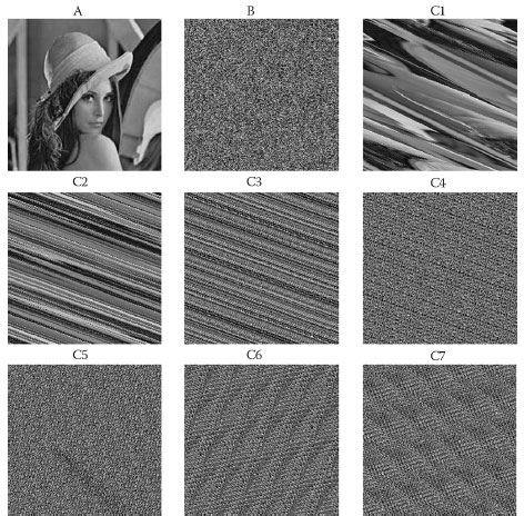
FIGURE 6.1 Image rearranged by and Algorithm 4 Arnold’s Cat map side-by-side. A is the original image, B is the rearranged image by Algorithm 4, and C1-C7 are the steps of Arnold’s Cat map rearrangement.

6.7    AN EXAMPLE IN IMAGE WATERMARKING

Algorithm 4 can be used with general watermarking techniques. The following example illustrates its use of applying LSB substitution for watermark. Even though this technique does not provide a robust watermark, the use of rearrangement does improve the security by making the watermark virtually undetectable. When pixel rearrangement is used and the adversary looks at the last two bits of the watermarked image, all one sees is random noise. The only way to see the watermark is to rearrange the pixels.

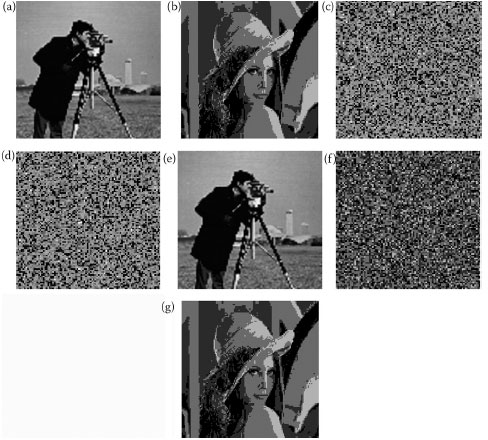
FIGURE 6.2 (a) The original Cameraman image, (b) the two most significant bits of Lena as the watermark, (c) the rearranged image of Cameraman using Algorithm 4, (d) the watermarked image of the rearranged image using LSB substitution, (e) the rearranged back of the preceding watermarked image using Algorithm 5, (f) the extracted 2 bits of LSB, and (g) the rearranged back of the preceding extracted image using Algorithm 5.

Figure 6.2 illustrates the advantages of using the rearrangement algorithm for image watermarking, where (a) is the original Cameraman image, (b) is the two most significant bits of the Lena image to be used as the watermark, (c) is the rearranged image of Cameraman using Algorithm 4, (d) is the watermarked image of the rearranged image using LSB substitution, (e) is the rearranged back of the preceding watermarked image using Algorithm 5, (f) is the extracted 2 bits of LSB , and (g) is the rearranged back of the preceding extracted image using Algorithm 5. Note that image (g) is exactly the same as the original watermark (b).

If the watermarking is performed without rearrangement, then the hidden watermark is easily detectible. By using the described algorithms, it is impossible to see the original watermark in image (f), which is random noise just like images (c) and (d). It is fairly difficult for the adversary to extract the original watermark, even though one knows that the watermark is hidden there. With sequential applications of Algorithm 4, the security could be enhanced to an arbitrary level, making watermark practically impossible to reconstruct for the adversary.

6.8    CONCLUSIONS

The described new method of rearranging image pixels for watermarking is based on the properties of Gaussian integers. It results in such a more random-looking image transformation that significantly improves the security of the embedded watermark. Moreover, its speed is much faster as compared with the Arnold cat map. The described algorithm is an easy-to-implement practical technique that would enhance the security of any watermarking algorithm. It is flexible enough to offer variable levels of security.

REFERENCES

Abramowitz, M. and Stegun, I. A. Handbook of Mathematical Functions. New York: Dover, 1964.

Al-Qaheri, H., Mustafi, A., and Banerjee, S.Digital watermarking using ant colony optimization in fractional Fourier domain. J. Inf. Hiding Multimedia Signal Process, 1(3), 220–240, 2010.

Arnold, V. I. and Avez, A. Ergodic Problems in Classical Mechanics. New York:Benjamin, 1968.

Berghel, H. and O’Gorman, L.Protecting ownership rights through digital watermarking. IEEE Comput. Mag., 29(7), 101–103, 1996.

Dawei, Z., Guanrong, C., and Wenbo, L. A chaos-based Robust wavelet-domain watermarking algorithm. Chaos Solitons Fractals, 22(1), 47–54, 2004.

El-Kassar, A., Rizk, M., Mirza, N., and Awad, Y. El-Gamal public-key cryptosystem in the domain of Gaussian integers. Int. J. Appl. Math., 7(4), 405–412, 2001.

El-Kassar, A. N., Haraty, R. A., Awad, Y. A., and Debnath, N. C. Modified Rsa in the domains of Gaussian integers and polynomials over finite fields. In Proceedings of the ISCA 18th International Conference on Computer Applications in Industry and Engineering, Dascalu, S. (ed.), pp.298–303. HI, USA: ISCA, 2005.

Elkamchouchi, H., Elshenawy, K., and Shaban, H. Extended Rsa cryptosystem and digital signature schemes in the domain of Gaussian integers. In Proceedings of the 8th International Conference on Communication Systems, pp. 91–95, IEEE Computer Society, 2002.

Huang, H.-C., Chen, Y.-H., and Abraham, A. Optimized watermarking using swarm-based bacterial foraging. J. Inf. Hiding Multimedia Signal Process, 1(1), 51–58, 2010.

Karatsuba, A. and Ofman, Y. Multiplication of many-digital numbers by automatic computers. Proceedings of the USSR Academy of Sciences, Vol. 145, pp. 293–294, 1962.

Knuth, D. E. The Art of Computer Programming. 3rd ed., Vol. 2, Redwood City, CA: Addison-Wesley, 1998.

Koval, A., Shih, F. Y., and Verkhovsky, B. S. A pseudo-random pixel rearrangement algorithm based on Gaussian integers for image watermarking. J. Inf. Hiding Multimedia Signal Process, 2(1), 60–70, 2010.

Lin, C.-C. and Shiu, P.-F. Highcapacity data hiding scheme for Dct-based images. J. Inf. Hiding Multimedia Signal Process, 1(3), 220–240, 2010.

Menezes, A. J., Oorschot, P. C. V., and Vanstone, S. A. Handbook of Applied Cryptography, Boca Raton, FL, USA: CRC Press, 1997.

Shih, F. Y. Digital Watermarking and Steganography: Fundamentals and Techniques. BocaRaton FL, USA: Taylor & Francis Group, CRC Press, Inc., 2008.

Verkhovsky, B. and Koval, A. Cryptosystem based on extraction of square roots of complex integers. In Fifth International Conference on Information Technology: New Generations (ITNG 2008), pp. 1190–1191. Las Vegas, NV, USA: IEEE Computer Society, 2008.

Verkhovsky, B. S. and Sadik, S. Accelerated search for Gaussian generator based on triple prime integers. J. Comput. Sci., 5(9), 614–618, 2009.

Wu, Y. and Shih, F. Y. Digital watermarking based on chaotic map and reference register. Pattern Recognit., 40(12), 3753–3763, 2007.

Yamamoto, K. and Iwakiri, M. Real-time audio watermarking based on characteristics of Pcm in digital instrument. J. Inf. Hiding Multimedia Signal Process, 1(2), 59–71, 2010.

Yantao, Z., Yunfei, M., and Zhiquan, L. A Robust Chaos-based Dct-domain watermarking algorithm. In Proceedings of the 2008 International Conference on Computer Science and Software Engineering, Yanshan University, China, pp. 935–938, IEEE Computer Society, 2008.

Ye, G. Image Scrambling encryption algorithm of pixel bit based on chaos map. Pattern Recognit.Lett., 31(5), 347–354, 2010.