4	Automatic Detection and Removal of Visible Image Watermarks
	Hong-Ren Su, Ya-Yun Cheng and Shin’ichi Lai

CONTENTS

4.1    Introduction

4.2    Visible Image Watermark

4.2.1    Watermark Embedding

4.2.2    Watermark Removal

4.3    Fourier-Based Image Registration

4.3.1    Rigid Transform Relationship Between Image and Fourier Domain

4.3.2    Moment Matching Approach to Estimating Rigid Transform Matrix

4.3.3    A Novel Fourier-Moment-Based Image Registration Algorithm

4.4    Iterative Refinement Process by a Distance Weighting

4.4.1    Binary Edge Image Data

4.4.2    Distance Weighting

4.4.3    Fourier-Based Image Registration Algorithm with Iterative Refinement

4.5    Visible Watermark Removal

4.5.1    Watermark Removal for Pictures

4.5.2    Watermark Removal for Text Images

4.6    Experiments and Discussions

4.7    Conclusions

References

4.1    INTRODUCTION

In recent years, widespread use of the Internet increased the exchange of information and knowledge. However, the accompanying copyright and ownership problems became very critical to the success of digital content distribution. In order to solve these problems for digital content, information-hiding techniques have become more and more important in many application areas. Electronic watermark, which is also called digital watermark, is a branch of information-hiding techniques and it is a common function in several famous photo-processing application programs. Digital watermarking can be roughly divided into two types—visible marking and invisible marking. The former is commonly used in academic theses and stock photos, and the latter is popular in commercial document sharing, copyright protection, and bill antifaking. Both these types have their own special requirements, such as easy embedding, copy prevention, hard removing, robustness against tempering, and preservation of original information.

The development of invisible watermarking technology has been almost two decades and there are two main approaches: one is the spatial-domain approach and the other is the frequency-domain approach. Van Schyndel et al. (1994) proposed an algorithm called Least-Significant Bits (LSB), which changes the least important bit to add the hiding information. Later, Pitas and Kaskalis (1995) and Pitas (1996) proposed a modified LSB method for information hiding, but the problem with this approach is that it is sensitive to image compression, noise adding, or other image attacking. The frequency-domain approach includes the discrete Cosine Transform (DCT)-based methods and discrete wavelet transform (DWT)-based methods. For example, Barni et al. (1998) proposed to embed a pseudo-random sequence of real numbers in a selected set of DCT coefficients, and Xia et al. (1998) proposed to add pseudo-random codes to the large coefficients at the high- and middle-frequency bands in the DWT of an image.

Sometimes watermarks need not be hidden in the digital contents, as some companies use visible watermarks, but most of the literature has focused on invisible (or transparent) watermarking. Visible watermarks overlaid on the original images or documents are strongly linked to the original watermarks and should be easy to recognize without blocking the original information. The critical point of the visible watermark is how to maintain the balance of watermark clearly visible yet difficult to move. Braudaway et al. (1996) used an analytic human perceptual models and varying pixel brightness to embed reasonably unobtrusive visible logos in color images, and an automatic way of adjusting the watermark intensity for a given image was presented in Rao et al. (1998) by using a texture-based human visual system (HVS) metric. Kankanhalli et al. (1999) worked in the DCT domain to classify DCT image blocks by image characteristics with the strength of the watermark in a block determined by its class. In Hu and Kwong (2001), they proposed a method to overcome the limitations of the DCT-domain-based methods and make the marking applied varied according to the features of the host images. The scaling factors are adaptively determined based on the luminance masking and local spatial characteristics of the host images.

Visible image watermark is commonly used to protect the copyright of documents and images. However, visible image watermark may cause problems for automatic understanding or analysis of the document or image contents, which is required for information or image retrieval. Thus, the visible watermark may need to be removed or modified, and the concept of reversible visible watermarks was proposed by IBM in 1997. The related literature has just rarely been reported. Pei and Zeng (2006) utilized independent component analysis to separate source images from watermarked and host images. Hu et al. (2006) presented a user-key-dependent removable visible watermarking system. Huang et al. (2007) proposed a copyright annotation scheme with both the visible watermarking and reversible data-hiding algorithms, and Liu and Tsai (2010) developed a lossless approach based on using deterministic one-to-one compound mappings of image pixel values for overlaying a variety of visible watermarks of arbitrary sizes on cover images.

In this chapter, we focus on the problems of detecting the visible watermarks from images and removing the watermarks to generate the watermark-free images. We will present our Fourier-based image alignment method with iterative refinement for the watermark detection. Subsequently, we describe how to remove the watermark from the image after the watermark is precisely detected. Some experimental results are given to show the performance of the proposed watermark detection and removal algorithm on real watermark documents and images.

4.2    VISIBLE IMAGE WATERMARK

Visible image watermark is commonly used to protect the copyright of documents and images. In general, most visible watermark embedding can be formulated as follows.

4.2.1    WATERMARK EMBEDDING

The visible image watermark embedding can be modeled as follows by Hu et al. (2006):

$\begin{array}{cc}{I}_{\text{t}}\left(x\right)=w_{\text{o}}\left(x\right)I_{\text{o}}\left(x\right)+w_{\text{w}}\left(x\right)I_{\text{w}}\left(x\right)& \text{for}x\in W\end{array}$

(4.1)

where W is the region of the watermark embedding, I_o(x) is the original image, I_w(x) is the watermark image, w_o(x) and w_w(x) are the associated weighting functions, and I_t(x) is the watermark-embedded image. Note that w_o(x) + w_w(x) = 1. The relationship of an original watermark I_w(y) and its transformed watermark I_w(x) can be modeled by a geometric affine transform given by x = Ay, where A is the affine transform matrix.

Generally speaking, w_o(x) and w_w(x) are usually set to constants inside the watermark area and the transformation A is usually the rigid transform with scaling, rotation, and translation. Figure 4.1 shows the typical visible watermark images with different weighting w_o. If w_o(x) and w_w(x) are not constant, the most common setting is as follows:

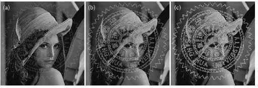
FIGURE 4.1 The watermark embedded images with (a) w_o = 0.8, (b) w_o = 0.5, and (c) w_o = 0.3.

$w_{\text{o}}\left(x\right)=\frac{I_{\text{w}}\left(x\right)}{I_{\text{o}}\left(x\right)+I_{\text{w}}\left(x\right)};w_{\text{w}}\left(x\right)=\frac{I_{\text{o}}\left(x\right)}{I_{\text{o}}\left(x\right)+I_{\text{w}}\left(x\right)}$

(4.2)

Combining Equations 4.1 and 4.2 leads to the following model:

$I_{\text{t}}\left(x\right)=\left(\frac{2}{I_{\text{o}}\left(x\right)+I_{\text{w}}\left(x\right)}\right)I_{\text{o}}\left(x\right)+I_{\text{w}}\left(x\right)$

(4.3)

This equation shows that the embedded image I_t(x) is proportional to the multiplication between I_o(x) and I_w(x). The main advantage of this embedding scheme is that no parameter is required to be adjusted.

For documents, the content can be segmented into two classes: that is, foreground and background. The foreground includes the texts or photos, and the background is always the white color area without anything, such as pdf or word files. In order to preserve the information for understanding, foreground will not be allowed to be modified. Thus the visible document watermarking can be defined as follows:

$I_{\text{t}}\left(x\right)=\{\begin{array}{cc}{I}_{\text{o}}\left(x\right)& x\in \text{foreground}\\ k{I}_{\text{w}}\left(w\right)& x\in \text{background}\cap \text{watermark region}\end{array}$

(4.4)

k is a scale factor for decreasing the intensity values of the watermark in the documents. Figure 4.2 depicts two examples of typical watermarked documents.

4.2.2    WATERMARK REMOVAL

Given two images, a watermark image and a watermarked document image, there are two steps in the watermark removal procedure. The first step is to detect the visible watermark from the watermarked image or document, and the second step is to remove the watermark to generate the watermark-free image. Figure 4.3 shows the system of the watermark removal. In the remainder of this chapter, we focus on giving a detailed description of watermark detection and water removal components. In the next section, we first review some previous works on Fourier-based image alignment methods, and then we present a novel Fourier-moment-based image alignment algorithm to precisely estimate the position, orientation, and scaling of the watermark from a watermarked image. Subsequently, we propose how to improve the image alignment accuracy under occlusion or outliers by introducing the distance weighting scheme in the proposed algorithm. In Section 4.4, we present how to remove watermark from a watermarked image after the watermark is precisely aligned. Finally, we show some experimental results, followed by some conclusions.

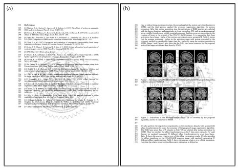
FIGURE 4.2 Two examples of watermarked documents: (a) watermarked document, (b) watermarked document containing images.

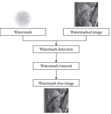
FIGURE 4.3 The system flow of watermark removal.

4.3    FOURIER-BASED IMAGE REGISTRATION

There have been several Fourier-based methods proposed for image registration in the past by De Castro and Morandi (1987), Bracewell et al. (1993), and Reddy and Chatterji (1996). All the Fourier-based methods have the advantages that it is robust to noise with low computational complexity and it can handle large motion. Unfortunately, the accuracy of the Fourier-based image registration methods is limited to the mapping of log-polar transform due to the spectrum interpolation error from the Cartesian plane to the log-polar plane for estimating rotation and scaling. The interpolation directly on the 2D Cartesian Fourier domain will result in error in the image registration. Thus, the log-polar transform is the primary challenge to improve the registration precision and the alignment range. Many modified Fourier-based image registration methods, like the log-polar method in Reddy and Chatterji (1996), unequally spaced Fourier transform by Averbuch et al. (2006), and multilayer fractional Fourier transform (MLFFT) by Pan et al. (2009), have been proposed to evaluate the log-polar transform more efficiently and reliably. MLFFT uses the fractional Fourier transform to create several spectrums with different resolutions from an image and sums them into one for the log-polar transform. This strategy makes the Fourier-based image registration more accurate than the other Fourier-based methods. However, MLFFT cannot go beyond the framework of the log-polar transform, and it just selects multiple spectrums from the fractional FFT to achieve better approximation.

In the next section, we will introduce a novel Fourier-based image registration algorithm without using the log-polar transform. This algorithm can be used in both rigid and affine registration, while the previous Fourier-based methods can only deal with the rigid alignment, which is composed of scaling, rotation, and translation. The proposed algorithm is based on the fact that the rigid transform between two images corresponds to a related rigid transform between their Fourier spectrums, whose energies are normally concentrated around the origin in the frequency domain. Thus, the moments for the corresponding Fourier spectrum distributions can be calculated as probability density functions. The novel registration algorithm is based on minimizing the relationship between the moments for the Fourier spectrums of the two images.

4.3.1    RIGID TRANSFORM RELATIONSHIP BETWEEN IMAGE AND FOURIER DOMAIN

Consider two images g(x, y) and h(x, y) and they are related by a rigid transformation, that is, $h\left(x,y\right)\hspace{0.17em}=\hspace{0.17em}g\left(r_0\cos {\text{θ}}_{0}x+r_0\sin {\text{θ}}_{0}y+c,\text{ -}{r}_0\sin {\text{θ}}_{0}x+r_0\cos {\text{θ}}_{0}y+f\right)$ with the rotation θ₀, scaling r₀and translation vector [c, f]^t. Assume the Fourier transforms of the image functions g(x, y) and h(x, y) be denoted by G(u, v) and H(u, v), respectively. Then, we can derive the following rigid relationship between the Fourier transforms G(u, v) and H(u, v) given as follows:

$G\left(u,v\right)=\frac{1}{r_0^2}{e}^{i\frac{[\left(c\cos {\text{θ}}_0-f\sin {\text{θ}}_0\right)u+\left(f\cos {\text{θ}}_0+c\sin {\text{θ}}_0\right)v]}{r_0}}H\left(\frac{\cos {\text{θ}}_{0}u+\sin {\text{θ}}_{0}v}{r_0},\frac{-\sin {\text{θ}}_{0}u+\cos {\text{θ}}_{0}v}{r_0}\right)$

(4.5)

By letting u′=(cos θ₀ + sinθθ₀ v)/r₀ and v′ = (–sinθ₀u + cosθ₀ v)/r₀ we have the relationship u = r₀(cosθ₀ u′ – sinθ₀v′) and v = r₀ (sinθu′ + cosθ₀ v′) Taking the absolute values on both sides of Equation 4.5, we have the rigid transformation relationship between the spectrums |G(u, v)| and |H(u, v)| as follows:

$\left|G\left(u,v\right)\right|=\frac{1}{\left|r_0^2\right|}\left|H\left(u^{\prime },v^{\prime }\right)\right|$

(4.6)

where

$\left[\begin{array}{c}u\\ v\end{array}\right]=\left[\begin{array}{cc}{r}_0\cos {\text{θ}}_0& -r_0\sin {\text{θ}}_0\\ r_0\sin {\text{θ}}_0& r_0\cos {\text{θ}}_0\end{array}\right]\left[\begin{array}{c}{u}^{\prime }\\ v^{\prime }\end{array}\right]$

(4.7)

Equations 4.6 and 4.7 show that the rigid transformation relationship in the amplitude of their Fourier spectrums only has two parameters, rotation Θ₀and scaling r₀. In order to evaluate them easily, Reddy and Chatterji (1996) proposed the log-polar transform from the Cartesian plane |G(u, v)| and |H(u, v)| into the log-polar plane M_g(log r, θ and M_h(log r, θ) in Equation 4.6 by letting u = r cos θ and v = r sin θ. Equation 4.6 can be rewritten as follows:

$M_{\text{g}}\left(\log r,\text{θ}\right)=\frac{1}{r_0^2}{M}_{\text{h}}\left(\log r-\log r_0,\text{θ}-{\text{θ}}_0\right)$

(4.8)

Equation 4.8 shows that the problem for estimating rotation and scaling is converted into a translation-like problem by taking the log-polar transform. Thus, the rotation and scaling can be determined as follows:

$\left(\log r_0,{\text{θ}}_0\right)=\arg \underset{\left(\log r,\text{θ}\right)}{\text{max}}\text{ real}\left(\text{IFT}\left\{\frac{\text{FT}\left(M_g\right)\text{conj}\left(\text{FT}\left(M_{\text{h}}\right)\right)}{\left|\text{FT}\left(M_g\right)\text{conj}\left(\text{FT}\left(M_{\text{h}}\right)\right)\right|}\right\}\right)$

(4.9)

where FT and IFT denotes the forward and inverse Fourier transform operators, respectively, and conj denotes the complex conjugate operator.

The rotation θ₀and scaling r₀ can be first estimated based on Equation 4.9 from the two Fourier spectrums FT(M_g) and FT(M_h) through the log-polar transform, and the remaining translation vector (c, f) can also be computed by transforming image g(x, y) with the transformation g′(x, y) = g(r₀cos θ₀x + r₀sin θ₀y, – r₀sin θ₀x + r₀cos θ₀) and determining the translation between g′(x, y) and h(x, y) from their cross-power spectrum. To be more specific, the translation vector is determined as follows:

$\left(c,f\right)\hspace{0.17em}=\hspace{0.17em}\arg \underset{\left(x,y\right)}{\text{max}}\text{ real}\left(\text{IFT}\left\{\frac{G^{\prime }\left(u,v\right)H^{*}\left(u,v\right)}{\left|G^{\prime }\left(u,v\right)H^{*}\left(u,v\right)\right|}\right\}\right)$

(4.10)

where G′(u, v) is the Fourier transform of g′(x, y), and H^*(u, v) is the complex conjugate of H(u, v).

4.3.2    MOMENT MATCHING APPROACH TO ESTIMATING RIGID TRANSFORM MATRIX

Owing to the interpolation error in the log-polar transform, we introduce the moment matching approach to estimate the rotation and scaling of the rigid transform in Equation 4.6 instead of using the log-polar transform. Let the Fourier spectrums of the 2D image functions f₁(x, y) and f₂(x, y) be denoted by F₁(u, v) and F₂(u, v), respectively. If f₁(x, y) and f₂(x, y) are related by a rigid transformation, then their Fourier spectrums are also related by the corresponding rigid transform, that is, |F₁(u, v)| = |F₂(u′, v′)|/r₀² with the relation between (u, v) and (u′, v′) given in Equation 4.7. We rewrite Equation 4.7 by a = r₀ cos θ₀ and b = r₀ sin θ₀ as follows:

$\left[\begin{array}{c}u\\ v\end{array}\right]=\left[\begin{array}{cc}a& -b\\ b& a\end{array}\right]\left[\begin{array}{c}{u}^{\prime }\\ v^{\prime }\end{array}\right]$

(4.11)

To determine the rigid transform parameters, a and b, we employ the moment matching technique to the Fourier spectrums F₁(u, v) and F₂(u, v). The (i + j) th-order moment for the Fourier spectrum |Fk(u, v)|, k = 1 or 2, is defined as

$m_{i,j}^{\left(k\right)}={\displaystyle \int {\displaystyle \int u^i{v}^j\left|F_k\left(u,v\right)\right|\text{d}u\text{d}v}}$

(4.12)

By coordinate substitution, we can derive the following equation:

${\text{m}}_{i,j}^{\left(1\right)}={\displaystyle \int {\displaystyle \int u^i{v}^j\left|F_1\left(u,v\right)\right|\text{d}u\text{ d}v}}$

(4.13)

$m_{i,j}^{\left(2\right)}={\displaystyle \int {\displaystyle \int {\left(a{u}^{\prime }-b{v}^{\prime }\right)}^i{\left(b{u}^{\prime }+a{v}^{\prime }\right)}^j\left|F_2\left(u^{\prime },v^{\prime }\right)\right|\text{d}{u}^{\prime }\text{d}{v}^{\prime }}}$

(4.14)

Thus, we have the following relationship between the first-order moments of the two Fourier spectrums from Equations 4.13 and 4.14.

$\left[\begin{array}{c}{m}_{1,0}^{\left(1\right)}\\ m_{0,1}^{\left(1\right)}\end{array}\right]=\left[\begin{array}{cc}a& -b\\ b& a\end{array}\right]\left[\begin{array}{c}{m}_{1,0}^{\left(2\right)}\\ m_{0,1}^{\left(2\right)}\end{array}\right]$

(4.15)

The 2D rigid transform parameters (a, b) can be estimated by minimizing the errors associated with the constraints in Equation 4.15 in a least-squares estimation framework as follows:

$a\text{=}\frac{m_{1,0}^{\left(1\right)}{m}_{1,0}^{\left(2\right)}+m_{0,1}^{\left(1\right)}{m}_{0,1}^{\left(2\right)}}{{\left(m_{1,0}^{\left(2\right)}\right)}^2+{\left(m_{1,0}^{\left(2\right)}\right)}^2}$

(4.16)

$b\text{=}\frac{m_{0,1}^{\left(1\right)}{m}_{1,0}^{\left(2\right)}-m_{1,0}^{\left(1\right)}{m}_{0,1}^{\left(2\right)}}{{\left(m_{1,0}^{\left(2\right)}\right)}^2+{\left(m_{0,1}^{\left(2\right)}\right)}^2}$

(4.17)

4.3.3    A NOVEL FOURIER-MOMENT-BASED IMAGE REGISTRATION ALGORITHM

In this section, we summarize the novel Fourier-moment-based image registration algorithm. The detailed procedure is given as follows:

1.  Compute the discrete Fourier transforms of two images h(x, y) and g(x, y) via FFT as Equation 4.6.

2.  Compute the first-order moments for the Fourier spectrums |H(u, v)| and |G(u, v)|.

3.  Determine the rigid transform parameters (a, b) in Equations 4.16 and 4.17 by minimizing the least-square errors associated with the moment matching constraints given in Equation 4.15.

4.  Transform the image g(x, y) with the rigid transform associated with the estimated parameters (a, b) and the transformed data are denoted by g′(x, y).

5.  Determine the translation from the cross-power spectrum of g′(x, y) and h′(x, y) based on Equation 4.10.

Compared with the previous Fourier-based image registration methods, the proposed Fourier-moment-based image registration approach has less time complexity and can provide higher accuracy, because it does not require the log-polar transform, which involves a computationally costly interpolation procedure on the log-polar plane and introduces errors in the interpolation.

4.4    ITERATIVE REFINEMENT PROCESS BY A DISTANCE WEIGHTING

In the previous section, we present a novel Fourier-moment-based image registration algorithm based on matching the moments with the Fourier spectrums of the image functions. To further improve the accuracy of the proposed image registration algorithm, especially to cope with the occlusion problem, we propose an iterative refinement process by introducing a distance weighting scheme into images, which is detailed in the following sections.

4.4.1    BINARY EDGE IMAGE DATA

Let a point set p(x, y) ∈ E, where E is the set of the Canny edge points, be extracted from an image h(x, y). Then the image h(x, y) is transformed into a binary image B(x, y) with values of the pixels set to 1 if they are edge points, and set to 0 otherwise.

$B\left(x\text{, }y\right)\text{=}\{\begin{array}{cc}1& \left(x\text{, }y\right)\in E\\ 0& \left(x\text{, }y\right)\notin E\end{array}$

(4.18)

4.4.2    DISTANCE WEIGHTING

The idea of improving the accuracy of the proposed Fourier-moment-based image registration algorithm under the occlusion or outlier problems is to assign an appropriate weight to each point p in the binary image such that the points without correspondences have very small weights and the points with proper correspondences have high weights in the binary image. In the previous definition of the binary image B given in Equation 4.18, the function has binary values to indicate the presence of data points. Since the point sets may contain some noise variation, we introduce a distance weighting to reduce the influence of the points without proper correspondences.

The distance for one data point p ∈ E₁ in the binary image B₁(x, y) to the other point set E₂ in the B₂(x, y) is defined as

$d\left(p,E_2\right)=\underset{q\in E_2}{\min }\Vert p-q\Vert$

(4.19)

Note that the distance for all data points in E₁ to E₂ can be efficiently computed by using the distance transform. Then, we define the weighting for each data point in E₁ to E₂ as follows:

$w\left(p,E_2\right)=\frac{{\text{σ}}^2}{{\text{σ}}^2+d^2\left(p,E_2\right)}$

(4.20)

To improve the correctness of the point correspondences, we employ both Euclidean and gradient distances to compute their corresponding weighting functions given in Equation 4.20. Thus, the total weighting w_t(p, E₂) is determined by the Euclidean weighting w_e(p, E₂) and the gradient distance weighting w_g(p, E₂), and they are defined as follows:

$w_{\text{t}}\left(p,E_2\right)=w_e\left(p,E_2\right)w_{\text{g}}\left(p,E_2\right)=\frac{{\text{σ}}_{\text{e}}^2}{{\text{σ}}_{\text{e}}^2+d_{\text{e}}^2\left(p,E_2\right)}\frac{{\text{σ}}_{\text{g}}^2}{{\text{σ}}_{\text{g}}^2+d_g^2\left(p,E_2\right)}$

(4.21)

where ${\text{σ}}_{\text{e}}^2\text{ and }{\text{σ}}_{\text{g}}^2$ are the parameters for the weighting function.

Thus, the binary image B₁ can be transformed into weighted image function Bw₁ as follows:

$B{w}_1\left(x,y\right)=\{\begin{array}{cc}{w}_{\text{t}}\left(\left(x,y\right),E_2\right)& \left(x,y\right)\in E_1\\ 0& \left(x,y\right)\cancel{\in }{E}_1\end{array}$

(4.22)

Similarly, the weight image function Bw₂ is defined as follows:

$B{w}_2\left(x,y\right)=\{\begin{array}{cc}{w}_{\text{t}}\left(\left(x,y\right),E_1\right)& \left(x,y\right)\in E_2\\ 0& \left(x,y\right)\notin E_2\end{array}$

(4.23)

In our algorithm, we first apply the proposed Fourier-moment-based image registration to the binary image B₁ and B₂ without using the distance weighting. The estimated rigid transform is applied to all points in E₁ to update the point set E₁. Then, the distance weighting is computed to produce the weighted image function Bw₁ and Bw₂ as given in Equations 4.22 and 4.23. The proposed Fourier-moment-based image registration algorithm is applied to find the rigid transformation between Bw₁ and Bw₂, and the estimation result is used to refine the rigid registration. This refinement process is repeated several times until convergence.

The iterative registration is very crucial to the robustness of the registration. If the first step cannot provide robust registration, then the iterative refinement will not converge to the correct registration results. The novel Fourier-based registration algorithm is robust even without the iterative refinement. It is because the Fourier transform of the image brings most of the energy to the low-frequency region in the Fourier domain, thus making the registration determined from the moments of the Fourier coefficients robust against noise which is normally considered to be mostly distributed in the high-frequency domain.

4.4.3    FOURIER-BASED IMAGE REGISTRATION ALGORITHM WITH ITERATIVE REFINEMENT

In this section, we summarize the Fourier-moment-based image registration algorithm with iterative refinement. The detailed procedure is given as follows:

1.  Generate the binary images B₁ and B₂ from the two images h(x) and g(x) as Equation 4.18.

2.  Compute the discrete Fourier transforms of B₁ and B₂ via FFT.

3.  Compute the first-order moments for the Fourier spectrums of B₁ and B₂ from Equations 4.13 and 4.14.

4.  Determine the rigid parameters by minimizing the least-square errors associated with the moment matching constraints given in Equation 4.15.

5.  Transform B₁ with the rigid transform associated with the estimated parameters (a, b) only and the transformed data are denoted by ${B^{\prime }}_1$.

6.  Determine the translation vector t between ${B^{\prime }}_1$ and ${B^{\prime }}_2$ via the cross-power spectrum method given in Equation 4.10.

7.  Shift the map ${B^{\prime }}_1$ with the translation vector t and compute the distance weighting from Equation 4.22 to form the weighting function Bw₁.

8.  Repeat step 2 through step 7 with the binary image replaced by the weighting functions computed in the previous step until the changes in the rigid transformation parameters are within a small threshold.

4.5    VISIBLE WATERMARK REMOVAL

According to the general model of visible watermark embedding, the production of watermarked text images and pictures is different; therefore, the methods of removing the watermarks to generate the watermark-free text and picture images are also different. We will describe the watermark removal methods for these two types of images subsequently in this section.

4.5.1    WATERMARK REMOVAL FOR PICTURES

Equation 4.1 shows the general model of watermark embedding. We consider the most common situation that w_o(x) and w_w(x) are set to a constant in all x positions belonging to the watermark area. If w_o(x) equals to c, then the model is transformed as follows:

$I_{\text{t}}\left(x\right)=c{I}_{\text{o}}\left(x\right)+\left(1-c\right)I_{\text{w}}\left(x\right)$

(4.24)

Equation 4.24 can be rewritten as follows:

$I_{\text{t}}\left(x\right)-I_{\text{W}}\left(x\right)=c\left(I_{\text{o}}\left(x\right)-I_{\text{W}}\left(x\right)\right)$

(4.25)

In a natural picture, it is very common that the intensity values of adjacent pixels are very close to each other. Thus, a small patch with watermarked area and its neighbors can be considered as having the similar intensity value in the watermark-free picture. Let I_t be the watermarked area and its neighbors be I_o. Figure 4.4 shows the intensity relationship between watermarked area and its neighboring region. After detecting the location and its geometric transformation of the watermark I_w in the watermarked image, we select the entire small patches with watermarked area and its neighbors, we can acquire many patch sets S = {S₁, S₂, S₃, …, S_n} and S_n = {I_o, I_t, I_w}. Then c can be solved by minimizing the least-square errors in Equation 4.25 between I_t – I_w and I_o – I_w using the entire patch S.

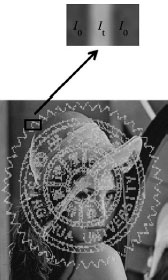
FIGURE 4.4 Intensity relationship between watermarked area and the neighboring region.

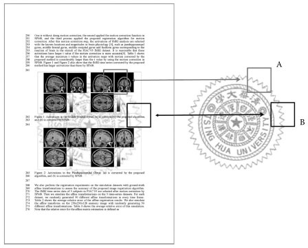
FIGURE 4.5 Detection of the watermark in the watermarked document image.

4.5.2    WATERMARK REMOVAL FOR TEXT IMAGES

The image in the watermarked text region is not changed by the watermark, which is visible only in the background of the document image and has smaller intensity values than the document image. After detecting the location and estimating the geometric transformation of the watermark I_w in the watermarked document image, we use the corresponding sliding windows both in watermarked document and in watermark. If the areas in the corresponding sliding windows are similar, such as the B area in Figure 4.5, intensity thresholding is simply applied to distinguish text and watermark regions based on their intensity distribution. If the areas in the corresponding sliding windows are very different, such as the A area in Figure 4.5, do nothing. A small sliding window is better to recover the watermark-free document image.

4.6    EXPERIMENTS AND DISCUSSIONS

There are two types of watermark removal experiments to demonstrate the effectiveness of the proposed algorithm in this section; namely, the picture and document image watermark removal. In the picture watermark removal experiments, the color Lena image (512 × 512) is used as the original picture with the watermark of Tsing Hua logo (146 × 139) imposed with random rigid geometric transform and different blending weight c values as shown in Figure 4.6. The documents are produced by ourselves and the same watermark of Tsing Hua logo is added with random rigid geometric transforms. The watermarked images and documents are printed by HP Color LaserJet CP2020 Series PCL6 and then the printed watermarked images and documents are scanned by HP Scanjet for practical watermark removal from paper-copy documents.

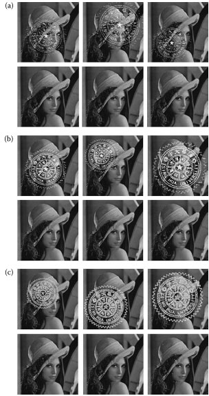
FIGURE 4.6 DFirst row: watermarked images with random watermark positions and scales. The blending weight c value is set to (a) 0.8, (b) 0.5, and (c) 0.3. Second row: the corresponding watermark-removed images by using the proposed algorithm.

When there is no noise or picture in the watermarked document image, the watermark removal can be simply accomplished by intensity thresholding if the watermark can be precisely detected and aligned from the image. However, there could be considerable noise corruption and image degradation after image scanning in practice. Figure 4.7 depicts an example of the document images before and after paper scanning. It is obvious that the image quality is greatly degraded after paper scanning. Figure 4.8 shows an example of the watermark removal result on a scanned document image containing pictures and texts by using the proposed watermark removal algorithm. It is clear that the proposed algorithm provides a satisfactory watermark removal result in this experiment.

FIGURE 4.7 (a) The ideal watermarked document and (b) the watermarked document image after paper scanning.

FIGURE 4.8 (a) A scanned watermarked document image and (b) the watermark-removed document image by using the proposed algorithm.

4.7    CONCLUSIONS

In this chapter, we presented a watermark removal algorithm to remove visible watermarks from picture or text images. Our algorithm is based on first applying a robust Fourier-moment-based image registration algorithm for watermark detection, followed by a watermark removal process for picture and text images. Experimental results demonstrate satisfactory watermark removal results for both the picture and document images. In the future, we aim to extend this robust Fourier-moment-based image registration algorithm to overcome more challenging watermark-embedding problems.

REFERENCES

Averbuch, A., Coifman, R. R., Donoho, D. L., Elad, M., and Israeli, M., Fast and accurate polar Fourier transform, Appl. Comput. Harmon. Anal., 21, 145–167, 2006.

Barni, M., Bartolini, F., Cappellini, V., and Piva, A., A DCT-domain system for robust image watermarking, Signal Process., 66(3), 357–372, 1998.

Bracewell, R. N., Chang, K. Y., Jha, A. K., and Wang, Y. H., Affine theorem for two-dimensional Fourier transform, Electron. Lett., 29(3), 304–309, 1993.

Braudaway, G. W., Magerlein, K. A., and Mintzer, F., Protecting publicly-available images with a visible image watermark, in Optical Security and Counterfeit Deterrence Techniques, Vol. 2659, R. L. van Renesse (ed.), San Jose, CA: ISandT and SPIE, pp. 126–133, 1996.

De Castro, E. and Morandi, C., Registration of translated and rotated images using finite Fourier transforms, IEEE Trans. Pattern Anal. Mach. Intell., 3, 700–703, 1987.

Hu, Y. and Kwong, S., Wavelet domain adaptive visible watermarking, IET Electron. Lett., 37(20), 1219–1220, September 2001.

Hu, Y. J., Kwong, S., and Huang, J., An algorithm for removable visible watermarking, IEEE Trans. Circuits Syst. Video Technol., 16(1), 129–133, 2006.

Huang, H. C., Chen, T. W., Pan, J. S., and Ho, J. H., Copyright protection and annotation with reversible data hiding and adaptive visible watermarking, Second International Conference on Innovative Computing, Information and Control, pp. 292–292, September 2007.

Kankanhalli, M. S., Rajmohan, R. and Ramakrishnan, K. R., Adaptive visible watermarking of images, in Proceedings of the IEEE Conference Multimedia Computing and Systems, vol. 1, pp. 568–573, 1999.

Liu, T. Y. and Tsai, W. H., Generic lossless visible watermarking—A new approach, IEEE Trans. Image Process., 19(5), 1224–1235, 2010.

Pan, W., Qin, K., and Chen, Y., An adaptable-multilayer fractional Fourier transform approach for image registration, IEEE Trans. Pattern Anal. Mach. Intell., 31(3), 400–413, 2009.

Pei, S. C. and Zeng, Y. C., A novel image recovery algorithm for visible watermarked images, IEEE Trans. Inf. Forensics Sec., 1(4), 543–550, 2006.

Pitas, I., A method for watermark casting on digital images, in Proceedings of the IEEE International Conference on Image Processing, vol. 3, pp. 215–218, 1996.

Pitas, I. and Kaskalis, P. H., Applying signatures on digital images, in Proceedings of the IEEE Workshop Nonlinear Image and Signal Processing, Neos Marmaros, Greece, pp. 460–463, June 1995.

Rao, A. R., Braudaway, G. W., and Mintzer, F. C., Automatic visible watermarking of images, Proceedings of the SPIE, Optical Security and Counterfeit Deterrence Techniques II, vol. 3314, pp. 110–121, 1998.

Reddy, B. S. and Chatterji, B. N., An FFT-based technique for translation, rotation, and scale-invariant image registration, IEEE Trans. Pattern Anal. Mach. Intell., 5(8), 1266–1270, 1996.

Van Schyndel, R. G., Tirkel, A. Z., and Osborne, C. F., A digital watermark, in Proceedings of the IEEE International Conference on Image Processing, vol. 2, pp. 86–90, November 1994.

Xia, X. G., Boncelet, C., and Arce, G., Wavelet transform based watermark for digital images, Opt. Express, 3(12), 497–511, 1998.