2	Discriminative Learning-Assisted Video Semantic Concept Classification
	Qiusha Zhu, Mei-Ling Shyu and Shu-Ching Chen

CONTENTS

2.1    Introduction

2.2    Related Work

2.2.1    Feature Selection

2.2.2    Classifier Learning

2.3    The Discriminative Learning Framework

2.3.1    Multiple Correspondence Analysis

2.3.2    MCA-Based Feature Selection Metric

2.3.3    MCA-Based Dual-Model Classification

2.4    Experiments and Results

2.5    Conclusions

References

2.1    INTRODUCTION

With the fast development and wide usage of digital devices, more and more people like to record their daily lives as videos and share them on websites such as YouTube, Yahoo Video, and Youku, to name a few. To get a better understanding of such video data and discover useful knowledge from them, effective and automatic multimedia semantic analysis becomes crucial. However, a manual analysis of multimedia data can be very expensive or simply not feasible when the time is limited or when the amount of data is enormous. Hence, the multimedia research community faces a major challenge: how to effectively and efficiently organize these videos. Data mining techniques have been successfully utilized to provide solutions to such a challenge. An example is video concept classification, which has been an attractive research focus in the past 10 years (Chen et al., 2006a; Shyu et al., 2008).

When extracting useful knowledge from the content of a video, it further brings up several issues such as semantic gap, imbalanced data, high-dimensional feature space, and varied qualities of the media (Chen et al., 2006b). Semantic gap refers to the gap between low-level visual features like color, texture, shape, etc., and high-level semantic concepts like boats, outdoors, streets, etc. (Hauptmann et al., 2007), which is produced by “the lack of coincidence between the information that one can extract from the visual data and the interpretation that the same data have for a user in a given situation” (Smeulders et al., 2000, p. 1353). A lot of effort has been put into bridging this semantic gap, but it is still difficult to conquer (Naphade et al., 2006). Next is the data imbalance issue that one usually encounters in video concept classification. It is very often that the number of videos of a particular concept we are interested in (called target/positive concept) is much less than the number of videos of the nontarget/negative concepts. The training process using a very small number of positive training data instances (i.e., data instances belonging to the target concept) and an extremely large number of negative (and usually noisy) training data instances (i.e., data instances belonging to nontarget concepts) typically results in poor or unsatisfactory classification performance. In the meantime, several new features are being developed to try to capture the semantic meaning of a video. For example, scale-invariant feature transform (SIFT) is one of the most well-known feature descriptors (Lowe, 2004), which uses the bag-of-words (BOW) model that usually represents an image in thousands of visual words. This could easily result in a highdimensional feature space and cause overfitting due to “curse of dimensionality.”

To overcome the aforementioned issues, one approach is to select a good representative subset of features from the original feature space. Such a process can reduce the feature space by removing irrelevant, redundant, or noisy features to improve classification performance and train a model to be more cost-effective. Feature selection can also preserve the semantics of the features compared with other dimensionality reduction techniques. Instead of altering the original representation of features like those based on projection (e.g., principal component analysis (PCA)) and compression (e.g., information theory) (Saeys et al., 2007), feature selection eliminates those features with little predictive information, keeps those with a better representation of the underlying data structure, and thus enhances the discriminative ability and semantic interpretability of the model. An effective representative subset of features should not contain (i) noisy features that decrease the classification accuracy, or (ii) irrelevant features that increase the computation time. Thus, a good feature selection method can intrinsically help video concept classification overcome these challenges. Feature selection techniques are also adopted in other areas as a pre-process step in order to improve model performance. An extensive comparison of 12 feature selection metrics for the high-dimensional domain of text classification was presented in (Forman, 2003), including chi-square measure (CHI), information gain (IG), document frequency, bi-normal separation (BNS), etc. These methods were evaluated on a benchmark of 229 text classification problem instances and the results showed that BNS was the top choice for evaluation criteria like accuracy, F1_score, and recall. Hua et al. (2009) compared several famous feature selection methods in the area of bioinformatics, including IG, gini index, t-test, sequential forward selection (SFS), and so on. Feature selection in this area is inevitable but quite challenging because biological technologies usually produce data with thousands of features but a relatively small sample size. Experiments on both synthetic and real data showed that none of these methods performed best across all scenarios, and revealed some trends relative to the sample size and relations among the features.

Another approach to overcome the challenges in multimedia semantic analysis is to improve inductive learning techniques and construct more powerful classifiers. Traditional classifiers like Decision Tree (DT), Native Bayes (NB), k-Nearest Neighbor (k-NN), and so on are considered as weak classifiers due to their low complexity, or unstable or poor performance. Multiple approaches have been proposed to build more powerful classifiers by combining weak classifiers. Boosting and bagging are two of the most popular combining strategies. The idea of bagging (Bressan, 1996) is to generate random bootstrap replicates from the training set, construct a classifier on each subset, and then combine them using the majority vote. The original boosting was proposed by Freund and Schapire (1997) which incrementally builds the final classifier by adding a new weak classifier at each step. When adding the weak classifiers, they are typically weighted in some way that is usually related to the weak classifiers’ accuracy. The data are reweighed too: samples that are mis-classified gain weights and samples that are classified correctly lose weights, so future weak classifiers could focus more on the “difficult” samples. After repeating this step a certain number of times, the final decision rule is constructed by weighting the weak classifiers at each step.

In this chapter, a new framework is proposed for video concept classification with the help of discriminative learning and multiple correspondence analysis (MCA) (Greenacre and Blaslus, 2006). Since features extracted from raw videos are numeric (e.g., feature “shot length” has many values: 2.5, 24.12, 6.0, etc.), as a straightforward approach, PCA has been used as a feature selection method in many literatures (Lu et al., 2007). However, it alters the original representation of the features by projecting all of them into a low-dimensional space and combining them linearly. MCA, on the other hand, is designed for nominal data (e.g., feature “outlook” has three items: “sunny,” “overcast,” and “rainy”), but has been proved to be able to effectively capture the correlation between a feature and a class (Lin et al., 2008a, Lin et al., 2008a,b; Zhu et al., 2010). Thus, MCA could be considered as a potentially better approach since, by choosing a subset from the original feature space, the semantic meaning of the feature is retained. The cosine value of the angle between a feature item and a class generated by MCA can indicate the strength of the relation between these two variables. In statistics, another property of a relation is reliability, which is called p-values or statistical significance. This motivates us to integrate correlation and reliability information represented by the cosine angle values and p-values to measure the relation between a feature and a class. Please note that the focus is on the problem of supervised learning, which means that the classification is carried out with the labels of the training data set known beforehand. Based on the metric that integrates the cosine angle values and p-values generated from MCA, a score is calculated for each feature with respect to each class, and therefore two feature lists are generated according to the ranking scores, one for each class. After employing MCA to select two discriminative sets of features from the original extracted features of the training data set, the features for the target concept are used to train the MCA-based positive model; while the features for the nontarget concepts are used to train the MCA-based negative model. To reach a better performance, a strategy is introduced that utilizes the dual-model for concept classification in the testing data set.

To evaluate the proposed discriminative learning framework, four widely used feature selection methods for supervised learning, namely the IG, CHI, correlation-based feature selection (CFS), and relief filter (REF) methods, available in WEKA (Witten and Frank, 2005) are used as a pre-processing step for five well-known classifiers, respectively: DT, Rule-based JRip (JRip), NB, Adaptive Boosting (Adaboost), and k-NN classifiers. The data used in the experiments is from TRECVID 2009 high-level feature extraction task, where the high-level features are actually the concepts to be detected in video shots. The overall experimental results demonstrate that the proposed framework which integrates the angle values and p-values generated from MCA together with the utilization of a dual model performs better than the other four feature selection methods in combination with the five classifiers in terms of the F1_scores.

This chapter is organized as follows. Related work is introduced in Section 2.2. The proposed framework is presented in Section 2.3, followed by an analysis of the experimental results in Section 2.4. Finally, Section 2.5 concludes the chapter.

2.2    RELATED WORK

Since feature selection and classification are two main components of the proposed framework, this section introduces related work in these two areas. It first describes different categories of supervised feature selection methods and then focuses on four commonly used ones: the IG, CHI, CFS, and REF. After feature selection, the training data set with selected features is used to train the classifiers which would classify the testing data set. Five well-known basic classifiers, namely DT, JRip, NB, Adaboost, and k-NN, are introduced, which are used in comparison with the proposed framework in Section 2.4.

2.2.1    FEATURE SELECTION

Depending on how it is combined with the construction of the classification model, supervised feature selection can be further divided into three categories: wrapper methods, embedded methods, and filter methods. Wrappers choose feature subsets with high prediction performance estimated by a specified learning algorithm which acts as a black box, and thus wrappers are often criticized for their massive amounts of computation which are not necessary. Similar to wrappers, embedded methods incorporate feature selection into the process of training a given learning algorithm, and thus they have the advantages of interacting with the classification model and meanwhile being less computationally intensive than wrappers. These two categories usually yield better classification results than the filter methods, since they are tailored to a specific classifier, but the improvements of the performance are not always significant because of “curse of dimensionality” and the fact that the specific-tuned classifiers may overfit the data. In contrast, filter methods are independent of the classifiers and can be scaled to high-dimensional datasets while remaining computationally efficient. In addition, filtering can be used as a pre-processing step to reduce space dimensionality and overcome the overfitting problem. Therefore, filter methods only need to be executed once, and then different classifiers can be evaluated based on the selected feature subsets.

Filter methods can be further divided two main subcategories. The first one is univariate methods which consider each feature with the class separately and ignore the interdependence between the features. Representative methods in this category include IG and CHI, both of which are widely used to measure the dependence of two random variables. IG evaluates the importance of features by calculating their IG with the class, but this method is biased to features with more values. In (Lee and Lee, 2006), a new feature selection method was proposed which selected features according to a combined criterion of IG and novelty of information. This criterion strives to reduce the redundancy between features, while maintaining IG in selecting appropriate features. In contrast, CHI calculates the chi-square statistics between each feature and the class, and a large value indicates a strong correlation between them. Although this method does not adhere strictly to the statistics theory because the probability of errors increases when a statistical test is used multiple times, it is applicable as long as it only ranks features with respect to their usefulness (Manning et al., 2008). Jiang et al. (2010) used the bag-of-visual-words features to represent keypoints in images for semantic concept detection. Feature selection applied the CHI to calculate the chi-square statistics between a specific visual word and a binary label of an image class, and eliminated those virtual words with chi-square statistics below a threshold. Extensive experiments on the TRECVID data indicated that the bag-of-visual-words features with an appropriate feature selection choice could produce highly competitive results.

The second subcategory is the multivariate methods which take features’ interdependence into account. However, they are slower and less-scalable compared with the univariate methods. CFS is one of the most popular methods. It searches among the features according to the degree of redundancy between them in order to find a subset of features that are highly correlated with the class, yet uncorrelated with each other (Hall, 2000). Experiments on natural datasets showed that CFS typically eliminated over half of the features, and the classification accuracy using the reduced feature set was usually equal to or better than the accuracy using the complete feature set. The disadvantage is that CFS degrades the performance of classifiers in cases where some eliminated features are highly predictive of very small areas of the instance space. This kind of cases could be frequently encountered when dealing with imbalanced data. Relief (Robnik-Sikonja and Kononenko, 1997) is another commonly used method whose idea is to choose the features that can be most distinguishable between classes. It evaluates the worth of a feature by repeatedly sampling an instance and considering the value of the given feature for the nearest instance of the same and different classes. However, relief lacks a mechanism to deal with the outlier instances, and according to Hua et al. (2009), it has worse performance than the univariate filter methods in most cases. Sun (2007) proposed an iterative relief (I-Relief) method by exploring the framework of the Expectation-Maximization algorithm. Large-scale experiments conducted on nine UCI datasets and six microarray datasets demonstrated that I-Relief performed better than relief without introducing a large increase in computational complexity.

According to the form of the outputs, the four aforementioned feature selection methods can also be categorized into ranker and nonranker. A nonranker method provides a subset of features automatically without giving an order of the selected features such as CFS. On the other hand, a ranker method provides a ranking list by scoring the features based on a certain metric, to which IG, CHI, and relief belong. Then different stopping criteria can be applied in order to get a subset from it. Most commonly used criteria include forward selection, backward elimination, bidirectional search, setting a threshold, genetic search, and so on.

2.2.2    CLASSIFIER LEARNING

There are several categories of inductive learning algorithms, such as Bayesian classifiers, trees, rules, and lazy classifiers. A popular data mining software WEKA has the implementation of several classification algorithms for each category. The five classifiers used in this chapter are listed as follows:

•  DT: J48 implements C4.5 (Quinlan, 1993) which is a tree structure where leaf nodes represent class labels and branches represent conjunctions of features that lead to those class labels. At each node of the tree, C4.5 chooses one attribute of the data that most effectively splits its set of samples into subsets enriched in one class or the other. Its criterion is the normalized IG (difference in entropy) that results from choosing an attribute for splitting the data. The attribute with the highest normalized IG is chosen to make the decision. The C4.5 algorithm then recurs on the smaller subtrees.

•  JRip: implements a propositional rule learner, repeated incremental pruning to produce error reduction (RIPPER), which was proposed by Cohen (1995). The algorithm contains a rule building stage and a rule optimization stage. The building stage repeats the rule grow and prune phase until the description length (DL) of the rule set and the examples is 64 bits greater than the smallest DL met so far, or there are no positive examples, or the error rate ≥ 50%.

•  Naive Bayes: John and Langley (1995) implemented the probabilistic Naive Bayes classifier and uses kernel density estimators to improve the performance if the normality assumption is grossly incorrect. In spite of its naive design and apparently over-simplified assumptions, naive Bayes classifier only requires a small amount of training data to estimate the parameters (means and variances of the variables) necessary for classification. Because independent variables are assumed, only the variances of the variables for each class need to be determined and not the entire covariance matrix.

•  Adaptive boost (Adaboost): Being considered as the best method for boosting (Freund and Schapire, 1997) which is used to combine weak classifiers, it assigns weights to the training data instances and iteratively combines the output of individual classifiers. AdaBoost is adaptive in the sense that subsequent classifiers built are tweaked in favor of those instances misclassi-fied by the previous classifiers. It can only handle nominal class problems and is sensitive to noisy data and outliers, but it often dramatically improves performance.

•  k-NN: is a type of instance-based learning or lazy learning which stores the training data instances and does no real work until the classification time. IBK (Aha and Kibler, 1991) is a k-nearest-neighbor classifier that finds the k training data instances closest in the Euclidean distance to the testing data instance. A testing data instance is classified by a majority vote of its neighbors, with the instance being assigned to the class most common amongst its k nearest training neighbors. Predictions from k neighbors can be weighted according to their distances to the testing data instance.

2.3    THE DISCRIMINATIVE LEARNING FRAMEWORK

The proposed discriminative learning framework is shown in Figure 2.1. It mainly contains two components: MCA-based feature selection and MCA-based dual-model classification. First, visual features are extracted from raw videos. In order to evaluate the framework, three-fold cross validation is adopted to split the data into training data set and testing data set. So the whole data set of each concept is randomly split into three sets with an approximately equal number of instances and equal positive to negative ratio. Each fold uses two of three sets as the training data set and the remaining one as the testing data set. Information entropy maximization (IEM) (Fayyad and Irani, 1993), a widely used supervised discretization based on minimum description length (MDL), also available in WEKA, is applied to the training set to discretize numeric features into nominal ones, and the same partitions are applied on the testing set.

Next, MCA-based feature selection is performed on the training set, which is enclosed in the dashed rectangular boxes labeled as (1). The correlation and reliability information generated from MCA are utilized to select two discriminative sets of features, one set for the positive class and the other one for the negative class. For the testing set, two sets of features same as the ones got from the training set are selected. The component of MCA-based dual-model classification is enclosed in the dashed rectangular boxes labeled as (2). It contains two MCA-based classifiers, a positive model and negative model, which are trained by the two sets of features from training set respectively, and a strategy is introduced to fuse these two models into a more powerful classifier to predict the class labels of the testing data instances. The following paragraphs are the detailed explanation about MCA theory used in the framework and the two components: MCA-based feature selection and MCA-based dual-model classification.

2.3.1    MULTIPLE CORRESPONDENCE ANALYSIS

Standard correspondence analysis (CA) is a descriptive/exploratory technique designed to analyze simple two-way contingency tables containing some measure of correspondence between the rows and columns. MCA can be considered as an extension of the standard CA to more than two variables (Greenacre and Blaslus, 2006). Meanwhile, it also appears to be the counterpart of PCA for nominal (categorical) data.

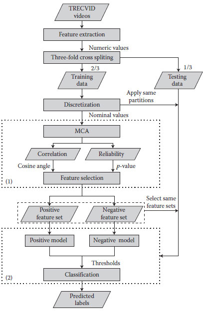
FIGURE 2.1 The proposed framework.

MCA constructs an indicator matrix with instances as rows and categories of valuables as columns. In order to apply MCA, each feature needs to be first discretized into several intervals/items or nominal values (called feature-value pairs in our study), and then each feature is combined with the class to form an indicator matrix. Assuming there are totally K features, and the kth feature has l_k feature-value pairs and the number of classes is m, then the indicator matrix is denoted by Z with size n × (l_k + m), where n is the number of data instances. Instead of performing on the indicator matrix which is often vary large, MCA analyzes the inner product of this indicator matrix, that is, Z^TZ, called the Burt Table which is symmetric with size (l_k + m) × (l_k + m). The grand total of the Burt Table is the number of instances which is n, then P = Z^T Z/n is called the correspondence matrix with each element denoted as P_ij. Let r_i and c_j be the row and column masses of P, that is, r_i = Σ_jP_ij and c_j = ΣP_ij. The centering involves calculating the differences (P_ij–r_ic_j) between the observed and expected relative frequencies, and normalization involves dividing these differences by $\sqrt{r_i{c}_j}$, leading to a matrix of standardized residuals $s_{ij}\hspace{0.17em}=\hspace{0.17em}\left(p_{ij}-r_i{c}_j\right)l\sqrt{r_i{c}_j}$. The matrix notation of this equation is presented in Equation 2.1.

$S=D_r^{-1/2}\left(P-r{c}^T\right)D_c^{1/2}$

(2.1)

where r and c are vectors of row and column masses, and D_r and D_c are diagonal matrices with these masses on the respective diagonals. Through singular value decomposition (SVD), S = UΣV^T where Σ is the diagonal matrix with singular values, the columns of U is called left singular vectors, and those of V are called right singular vectors. The connection of the eigenvalue decomposition and SVD can be seen through the transformation in Equation 2.2:

$S{S}^T=U{{\displaystyle \Sigma }}^{\text{}}{V}^{T}V{\displaystyle \Sigma U^T}=U{\displaystyle \Sigma {}^2{U}^T}=U\text{Λ}{U}^T$

(2.2)

Here,Λ = Σ²is the diagonal matrix of the eigenvalues, which is also called principal inertia. Thus, the summation of the principal inertia is the total inertia which is also the amount that quantifies the total variance of S. The geometrical way to interpret the total inertia is that it is the weighted sum of squares of principal coordinates in the full S-dimensional space, which is equal to the weighted sum of squared distances of the column or row profiles to the average profile. This motivates us to explore the distance between feature-value pairs and classes represented by the rows of principal coordinates in the full space. Since in most cases, over 95% of the total variance can be captured by the first two principal coordinates, the chi-square distance between a feature-value pair and a class can be well represented by the Euclidean distance between them in the first two dimensions of their principal coordinates. Thus, a geometrical representation, called the symmetric map, can visualize a feature-value pair and a class as points in the two-dimensional map.

As shown in Figure 2.2, a nominal feature F_k with three feature-value pairs corresponds to three points in the map, namely $F_k^1,F_k^2$, and $F_k^3$ respectively. Considering a binary class, it is represented by two points lying in the x-axis, where C₁ is the positive class and C₂ is the negative class. Take $F_k^1$ as an example. The angle between $F_k^1$ and C₁ is $a_{k1}^1$, and the distance between them is $d_{k1}^1$, the angle and distance of $F_{k1}^1$ with C₂ is $a_{k2}^1$ and $d_{k2}^1$. Similar to standard CA, the meaning of $a_{k2}^1$and $d_{k2}^1$ in MCA can be interpreted as follows:

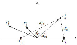
FIGURE 2.2 The geometrical representation of MCA.

•  Correlation: The cosine value of the angle between a feature-value pair and a class in the symmetric map indicates the strength of their relation. It represents the percentage of the variance that the feature-value pair point is explained by the class point. A larger cosine value which is equal to a smaller angle indicates a larger correlation between the feature-value pair and the class.

•  Reliability: As stated before, chi-square distance could be used to measure the dependence between a feature-value pair point and a class point. Here, a derived value from chi-square distance called the p-value is used because it is a standard measure of the reliability of a relation, and a smaller p-value indicates a higher level of reliability.

More technically, p-value represents a decreasing index of the reliability of a result. The higher the p-value, the less we can believe that the observed relation between variables in the sample is a reliable indicator of the relation between the respective variables in the population. Assume that the null hypothesis H₀ is true, which here represents there is no relation between a feature-value pair and a class. Thus, p-value tells us the probability of error involved in rejecting H₀. Generally, one rejects H₀ if the p-Value is smaller than or equal to the significance level, which means the smaller the p-value, the higher possibility of the correlation between a feature-value pair and a class is true. p-value can be calculated through the chi-square cumulative distribution function (CDF) and the degree of freedom is (number of feature-value pairs – 1) × (number of classes – 1). For example, the chi-square distance between $F_k^1$ and C₁ is$d_{k1}^1$ and their degree of freedom is (3 – 1) × (2 – 1), and then their p-value is 1 – cdf $\left(d_{k1}^1,2\right)$. Therefore, correlation and reliability are from differentpoints of view, and can be integrated together to represent the relation between a feature and a class.

2.3.2    MCA-BASED FEATURE SELECTION METRIC

For a feature F_k, the cosine angle values and p-values of each feature-value pair of this feature to the positive and negative classes are calculated, corresponding to correlation and reliability, respectively. If the angle of the jth feature-value pair $F_k^j$ with the positive class is < 90 degrees, it indicates this feature-value pair is correlated with the positive class, and negatively correlated with the negative class to the same degree, so Equation 2.3 stands.

$\cos \left(a_{k1}^j\right)\hspace{0.17em}=\hspace{0.17em}-\cos \left(a_{k2}^j\right)$

(2.3)

For p-value, since a smaller p-value indicates a higher reliability, $F_k^j$ can be used as the error of accepting the correlation between $F_k^j$ and C₁, and $p_{k2}^j$ is the error of accepting the correlation between $p_k^j$ and C₂, except for the situation of Jeffrey-Lindley paradox (Lindley, 1957). This paradox describes a situation when the p-value is very close to zero but the probability of the correlation being true is very close to zero as well. Such scenario could happen when the prior distribution is the sum of a sharp peak at H₀ with probability p and a broad distribution with the rest of the probability 1 – p. In our experiments (to be discussed in Section 2.4), it occurs when the count of the cross-table constructed by the feature-value pairs and the classes is < 1% of the count of the corresponding class, which also makes sense since a rare occurrence can be considered as a “fluke.”

After getting the correlation and reliability information of each feature-value pair with the class from the geometrical representation from MCA, a score can be calculated for each feature. Assume there are totally n data instances with K features. For the kth feature with l_k feature-value pairs, the angles and p-values for the jth feature-value pair are $a_{k1}^j$ and $p_{k1}^j$for the positive class C₁, and $a_{k2}^j$and $p_{k2}^j$for the negative class, respectively. Considering Equation 2.3, $\left|\cos \left(a_{k1}^j\right)\right|$ or $\left|\cos \left(a_{k2}^j\right)\right|$ can be used to indicate the correlation between $F_k^j$ with either C₁ or C₂, but and $p_{k1}^j$ is not equal to and $p_{k2}^j$. Thus, there are two scores for each feature, one is for the positive class pos_score_kand one is for the negative class neg_score_k · $\left|\cos \left(a_{k1}^j\right)\right|$ is added to the feature score if its p-value is smaller than a threshold, which is defined in Equation 2.4a as TH(p₁) for C₁, and in Equation 2.4b as TH(p₂) for C₂, where $\underset{{\Sigma }_{l_k}}{\text{mediam}}\left(p_{k1}\right)$ and $\underset{{\Sigma }_{l_k}}{\max }\left(p_{k1}\right)$ is the median and maximum of all the p-values related to C₁(Σl_k, k is from 1 to K), and TH(p₁) is set to the median of these two values based on the empirical study.

$TH\left(p_1\right)\text{ =}\left(\underset{{\text{Σ}}_{lk}}{\text{median}}\left(p_{k1}\right)\text{, }\underset{{\text{Σ}}_{lk}}{\text{max}}\left(p_{k1}\right)\right)$

(2.4a)

$TH\left(p_2\right)\text{ = median }\left(\underset{{\text{Σ}}_{lk}}{\text{median}}\left(p_{k2}\right)\text{, }\underset{{\text{Σ}}_{lk}}{\text{max}}\left(p_{k2}\right)\right)$

(2.4b)

The following pseudo-code is developed to integrate the angle value and p-value as a feature-scoring metric (considering Jeffrey-Lindley paradox). According to the scores of the features, two ranking lists can be generated in descending order of the scores, one list of features is specially discriminative to positive class while the other list of features is specially discriminative to negative class. Forward selection is adopted to select the best feature subset for each model. It starts with an empty feature subset, and then at each time, it takes out the feature at top of the ranking list and adds it to the feature subset which is evaluated by the model. Repeat this until all the features in the ranking list are added into the feature subset. The subset that produces the best F1_score is selected as the feature subset for that model.

1 for k = 1 to K

2  pos_score_k = 0;

3  neg_score_k = 0;

4  for j = 1 to l_k

5   if $p_{k1}^j<TH\left(p_1\right){\text{ count}}_{k1}^j\text{ >}0.01\times \text{n}$

6    $\text{pos}\_{\text{score}}_{\text{k}}+=\left|\cos \left({\text{a}}_{k1}^j\right)\right|;$

7   end

8   if $p_{k1}^j>TH\left(p_1\right)$ and ${\text{count}}_{k2}^j>0.01\times \text{n}$

9    $\text{neg}\_{\text{score}}_{\text{k}}+=\left|\cos \left({\text{a}}_{k1}^j\right)\right|;$

10   end

11  end

12  pos_score_k = pos_score_k/l_k;

13  neg_score_k = neg_score_k/l_k;

14 end

2.3.3    MCA-BASED DUAL-MODEL CLASSIFICATION

A data instance that consists of a certain feature-value pair from each feature can be viewed as a transaction in the database. For the training set, a transaction is an instance without the class label, shown in Table 2.1, each row is a transaction. Cosine value of the angles can be used as weights of feature-value pairs to indicate their correlation with the classes. If the value is close to 1, then this feature-value pair is highly correlated to the positive class. On the contrary, if the value is close to –1, then the feature-value pair is highly correlated to the negative class. If it is close to 0, it means this feature-value pair does not have much discriminative ability. Based on this, for instance, if the sum of all weights of its feature-value pairs is a relatively large positive value, the label of this instance is probably positive, vice versa. Thus, for the training set with K features, a transaction weight for each of its data instances TW_i can be calculated, denoted in Equation 2.5, where j is a value between 1 to l_k, and a threshold can be set that optimizes the classifier. For a testing data instance, its transaction weight is first calculated in the same way, and then it is compared with the threshold. If it is smaller than the threshold, then it is predicted as a negative instance, otherwise predicted as a positive instance.

$T{W}_i={\displaystyle \sum _{k=1}^K\cos \left(a_k^j\right)}$

(2.5)

TABLE 2.1
Transactions of the Training Data Set

Feature 1	Feature 2	…	Feature K
$F_1^3$	$F_1^2$	…	$F_4^{\mathrm{K}}$
$F_1^1$	$F_2^1$	…	$F_{\mathrm{K}}^1$
…	…	…	…

After the feature selection phase, two subsets of features are selected to train two classifiers, which are based on MCA transaction weights. In the above Equation 2.5, K is adjusted to the number of features in the selected feature set for each classifier. In addition, only positive correlated feature-value pairs are considered, which means for the positive model, $\cos \left(a_k^j\right)$ is added to TW_i only if $\cos \left(a_k^j\right)>0$. On the opposite, for the negative model, $\cos \left(a_k^j\right)$) is added to TW_i only if $\cos \left(a_k^j\right)<0$. In this way, the weights of the feature-value pairs of a transaction will not cancel each other out. A threshold for the positive model pos_TH and a threshold for the negative model neg_TH need to be tuned, respectively, which involve finding two parameters: t₁ and t₂, shown in Equations 2.6a and 2.6b. Based on the dataset and empirical studies, t₁ is set to 1 while t₂ is set to 0.06 in the experiment in Section 2.4.

$pos\_TH=pos\_mean+t_1\times pos\_std$

(2.6a)

$neg\_TH=neg\_mean+t_1\times neg\_std$

(2.6b)

However, since the number of features selected for each classifier is different, normalization is needed to be applied to both models to ensure the transaction weights lie in the same range and suitable for later processes. Z-score normalization is adopted here. Thus, after normalization, pos_TH is equal to t₁, while neg_TH is equal to t₂. A strategy is introduced to fuse these two classifiers into a more powerful one. When a testing data instance i comes, two transaction weights are calculated, one by each model: pos_TW_i and neg_TW_i.

The above pseudo-code presents the rules to classify this testing data instance. Note that |pos_ TW_i – pos_TH| is the distance to the threshold of the positive model, and |neg_ TW_i– neg_ TH| is the distance to the negative model, they are able to compare with each other after the normalization applied before.

2.4    EXPERIMENTS AND RESULTS

To evaluate the proposed framework, experiments are conducted using 10 concepts from TRECVID 2009. Each concept data set has more than 12,000 instances and 48 low-level visual features. These 10 concepts range from slightly imbalanced (e.g., hand) to highly imbalanced (e.g., traffic-intersection) with positive to negative (P/N) ratio as shown in Table 2.2. Five classifiers, namely DT, JRip, NB, Adaboost which uses DT as the basic classifier, and k-NN where k is set to 3, are used as comparisons, and the input of these five classifiers are the features selected by four feature selection methods: IG, CHI, CFS, and REF. So there are 20 combinations used as comparisons of the proposed framework, each with one feature selection method combined with one classifier. Precision (pre), recall (rec), and F1_score (F1), which is the harmonic mean of precision and recall, are adopted as the evaluation metrics for classification, their calculations are defined in Equations 2.7a, 2.7b, and 2.7c, where TP, FP, and FN represent true positive, false positive, and false negative, respectively. The final result of a classifier is the average classification results of three folds.

TABLE 2.2
Concepts to Be Evaluated

No.	Concept Name	P/N Ratio
1	Chair	0.07
2	Traffic-intersection	0.01
3	Person-playing-musical-instrument	0.04
4	Person-playing-soccer	0.01
5	Hand	0.25
6	People-dancing	0.02
7	Night-time	0.06
8	Boat-ship	0.06
9	Female-human-face	0.10
10	Singing	0.07

TABLE 2.3
Classification Results of Adaboost

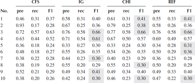
TABLE 2.4
Classification Results of DT

$\text{precision}\hspace{0.17em}=\hspace{0.17em}\frac{TP}{TP+FP}$

(2.7a)

$\text{recall}\hspace{0.17em}=\hspace{0.17em}\frac{TP}{TP+FP}$

(2.7b)

$F1\_\text{score}\hspace{0.17em}=\hspace{0.17em}2\times \frac{\text{precision}\times \text{recall}}{\text{precision}+\text{recall}}$

(2.7c)

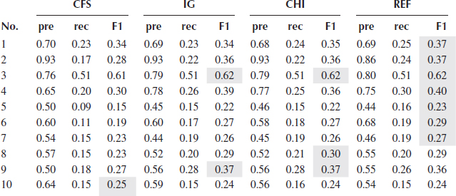
Tables 2.3, 2.4, 2.5, 2.6, 2.7 show the precision, recall, and F1_score of five classifiers using four different feature selection methods. Since all the selection metrics only generate the ranking list of the features except CFS which directly provides the selected features, forward selection mentioned in Section 2.3.2 is used to find the feature subset that gives the best performance of a classifier, evaluated by F1_score. For each feature selection method, the best performance produced by a feature subset is recorded in the tables.

TABLE 2.5
Classification Results of JRip

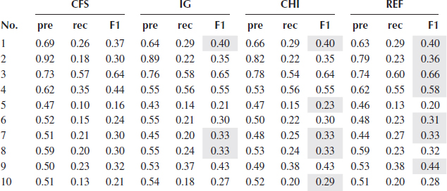
TABLE 2.6
WClassification Results of k-NN

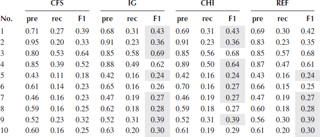
Table 2.8 shows the performance of the proposed framework (denoted as MCA). The same forward selection is used in the two models to select the feature sets. As can be seen from Figure 2.3 which shows the F1_scores of MCA and the best F1_scores from the five tables (cells shaded gray) of each classifier for all 10 concepts, MCA performs the best in all 10 concepts regarding to F1_score which is the most important metric taking both precision and recall into account, followed by NB, k-NN, and Adaboost. DT performs the worst. MCA outperforms the second best result in an average of 4% in F1_scores, and outperforms the worst one in an average of 15%.

TABLE 2.7
Classification Results of NB

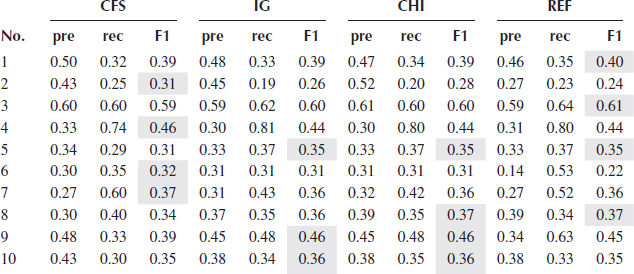
TABLE 2.8
Classification Results of the Proposed Framework

	MCA
No.	pre	rec	F1
1	0.58	0.41	0.48
2	0.62	0.35	0.45
3	0.77	0.69	0.73
4	0.82	0.63	0.71
5	0.58	0.27	0.37
6	0.41	0.34	0.37
7	0.49	0.35	0.41
8	0.55	0.29	0.38
9	0.40	0.68	0.50
10	0.53	0.36	0.43

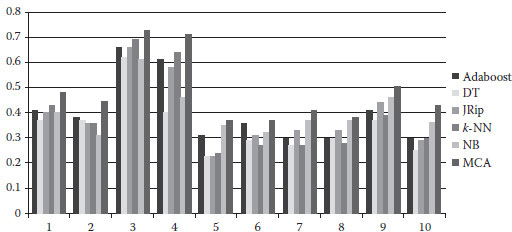
FIGURE 2.3 Comparison of best F1_scores among six classifiers.

In terms of classification performance on the features selected by the four feature selection methods, CFS usually has the worst results except when using NB, four out of 10 concepts achieve the best F1_scores. The performance of IG and CHI are quite similar, and REF produces a slightly better result in DT compared with IG and CHI. In general, for each classifier, the margin of the performance resulted by these three methods is quite small.

2.5    CONCLUSIONS

In this chapter, a new dual-model discriminative learning framework for video semantic classification is proposed to address the challenges such as semantic gap, imbalanced data, and high-dimensional feature space in automatic multimedia semantic analysis. Our proposed framework utilizes MCA to calculate the relation between a feature-value pair and a class. The correlation and reliability information, represented by the cosine angles values and p-values, respectively, are integrated into a single metric to score the features. In addition, the correlation information is reutilized to build two models based on the transaction weights. A strategy is also pro-posed to fuse these two models into a more powerful classifier. The results of the experiments on 10 concepts from TRECVID 2009 demonstrate that the proposed framework shows promising results compared with 20 combinations of five well-known classifiers and four widely used feature selection methods.

AREFERENCES

Aha, D. and Kibler, D., Instance-based learning algorithms, Machine Learning, 6, 37–66, 1991.

Bressan, M., Bagging predictors, Machine Learning, 24(3), 123–140, 1996.

Chen, S.-C., Chen, M., Shyu, M.-L., Zhang, C., and Chen, M., A multimodal data mining framework for soccer goal detection based on decision tree logic, International Journal of Computer Applications in Technology, Special Issue on Data Mining Applications, 27(4), 312–323, 2006a.

Chen, S.-C., Chen, M., Shyu, M.-L., and Wickramaratna, K., Semantic event detection via temporal analysis and multimodal data mining, IEEE Signal Processing Magazine, Special Issue on Semantic Retrieval of Multimedia, 23, 38–46, 2006b.

Cohen, W. W., Fast Effective Rule Induction, in International Conference on Machine Learning, Tahoe City, California, USA, pp. 115–123, 1995.

Fayyad, U. M. and Irani, K. B., Multi-interval discretization of continuous-valued attributes for classification learning, in Proceedings of International Joint Conference on Artificial Intelligence, Chambéry, France, pp. 1022–1027, 1993.

Forman, G., An extensive empirical study of feature selection metrics for text classification, The Journal of Machine Learning Research, 3, 1289–1305, 2003.

Freund, Y. and Schapire, R. E., A decision-theoretic generalization of on-line learning and an application to boosting, Journal of Computer and System Sciences, 55(1), 119–139, 1997.

Greenacre, M. J. and Blaslus, J., Multiple Correspondence Analysis and Related Methods. Chapman and Hall/CRC, London, UK, 2006.

Hall, M. A., Correlation-based feature selection for discrete and numeric class machine learning, in Proceedings of International Conference on Machine Learning, Stanford, California, USA, pp. 359–366, 2000.

Hauptmann, A. G., Yan, R., Lin, W., Christel, M. G., and Wactlar, H. D., Can high-level concepts fill the semantic gap in video retrieval? A case study with broadcast news, IEEE Transactions on Multimedia, 9(5), 958–966, 2007.

Hua, J., Tembe, W. D., and Dougherty, E. R., Performance of feature selection methods in the classification of high-dimension data, Pattern Recognition, 42(3), 409–424, 2009.

Jiang, Y. G., Yang, J., Ngo, C. W., and Hauptmann, A. G., Representations of keypoint-based semantic concept detection: A comprehensive study, IEEE Transactions on Multimedia, 12(1), 42–53, 2010.

John, G. H. and Langley, P., Estimating continuous distributions in Bayesian classifiers, in Conference on Uncertainty in Artificial Intelligence, Montreal, Quebec, Canada, pp. 338–345, 1995.

Lee, C. and Lee, G. G., Information gain and divergence-based feature selection for machine learning-based text categorization, Information Processing and Management, 42(1), 155–165, 2006.

Lin, L., Ravitz, G., Shyu, M.-L., and Chen, S.-C., Correlation-based video semantic concept detection using multiple correspondence analysis, in Proceedings of IEEE International Symposium on Multimedia, Berkeley, California, USA, pp. 316–321, 2008a.

Lin, L., Ravitz, G., Shyu, M.-L., and Chen, S.-C., Effective feature space reduction with imbalanced data for semantic concept detection, in Proceedings of IEEE International Conference on Sensor Networks, Ubiquitous, and Trustworthy Computing, Taichung, Taiwan, R.O.C., pp. 262–269, 2008b.

Lindley, D., A statistical paradox, Biometrika, 44(1–2), 187–192, 1957.

Lu, Y., Cohen, I., Zhou, X. S., and Tian, Q.Feature selection using principal feature analysis. In Proceedings of the International Conference on Multimedia, Augsburg, Germany, pp. 301–304, 2007.

Lowe, D., Distinctive image features from scale-invariant keypoints, International Journal of Computer Vision, 2(60), 91–110, 2004.

Manning, D. C., Raghavan, P., and Schutze, H., Text classification and Naive Bayes, Introduction to Information Retrieval, Cambridge University Press, Cambridge, UK, pp. 253–287, 2008

Naphade, M., Smith, J. R., Tesic, J., Chang, S.-F., Hsu, Wu., Kennedy, L., Hauptmann, A., and Curtis, J., Large-scale concept ontology for multimedia, IEEE Multimedia Magazine, 13(3), 86–91, 2006.

Quinlan, R., C4.5: Programs for Machine Learning, Morgan Kaufmann Publishers, San Francisco, CA, 1993.

Robnik-Sikonja, M. and Kononenko, I., An adaptation of relief for attribute estimation in regression, in International Conference on Machine Learning, Nashville, Tennessee, USA, pp. 296–304, 1997.

Saeys, Y., Inza, I., and Larranaga, P., A review of feature selection techniques in bioinformatics, Bioinformatics, 23(19), 2507–2517, 2007.

Shyu, M.-L., Xie, Z., Chen, M., and Chen, S.-C., Video semantic event/concept detection using a subspace-based multimedia data mining framework, IEEE Transaction on Multimedia, 10(2), 252–259, 2008.

Smeulders, A. W. M., Worring, M., Santini, S., Gupta, A., and Jain, R., Content-based image retrieval: The end of the early years, IEEE Transaction Pattern Analysis and Machine Intelligence, 22, 1349–1380, 2000.

Sun, Y., Iterative relief for feature weighting: Algorithms, theories, and applications, IEEE Transactions on Pattern Analysis and Machine Intelligence, 29(6), 1035–1051, 2007.

Witten, I. H. and Frank, E., Data Mining: Practical Machine Learning Tools and Techniques, 2nd ed. Morgan Kaufmann, San Francisco, CA, 2005.

Zhu, Q., Lin, L., and Shyu, M.-L., Feature selection using correlation and reliability based scoring metric for video semantic detection, In Proceedings of IEEE International Conference on Semantic Computing, Pittsburgh, PA, USA, pp. 462–469, 2010.