8	Q Watermarking Based on Local Binary Pattern Operator
	Wenyin Zhang and Frank Y. Shih

CONTENTS

8.1    Introduction

8.2    LBP Operator and its Extensions

8.2.1    Original LBP Operators

8.2.2    Extensions of Original LBP Operators

8.2.3    Other LBP Operators

8.3    Spatial Watermarking Based on LBP Operators

8.3.1    Definitions on a (P, R) Local Region

8.3.2    Watermark-Embedding Algorithm

8.3.3    Watermark Extraction Algorithm

8.4    Experimental Results and Analysis

8.5    Multilevel Watermarking Based on LBP Operators

8.5.1    Double-Level Watermarking

8.5.2    Extension to Multilevel Watermarking

8.6    Conclusions

References

8.1    INTRODUCTION

The successes of the Internet and digital consumer devices have been profoundly changing our society and daily lives by making the capture, transmission, and storage of digital data extremely easy and convenient. However, this raises large concern on how to secure these data and prevent unauthorized modification. This issue has become problematic in many areas, such as copyright protection including (Schyndel et al., 1994; Pitas, 1996; Swanson et al., 1996; Xia et al., 1997), content authentication (Yeo and Kim, 2001; Cvejic and Tujkovic, 2004), hiding of information (Tanaka et al., 1990), and covered communications (Chen and Wornell, 2001). Digital watermarking technologies are considered to be an effective means to address this issue. Many researchers have developed various algorithms of digital watermarking methods which intend to embed some secret data (called watermark) in digital content to mark or seal the digital data content, such as (Cox et al., 1997; Podilchuk and Zeng, 1998; Kaewkamnerd and Rao, 2000; Piva et al., 2000; Reed and Hannigan, 2002; Bas et al., 2003; Shih and Wu, 2003; Shih, 2008; Tsui et al., 2008; Sachnev et al., 2009; Wei and Ngan, 2009; Yang et al., 2009; Luo et al., 2010; Wu and Cheung, 2010). The watermark embedded into a host image is such that the embeddinginduced distortion is too small to be noticed. At the same time, the embedded watermark must be robust enough to withstand common degradations or deliberate attacks.

During the last 20 years, digital watermarking techniques have achieved considerable progress, from the spatial domain to the transformed domain, from robustness to fragileness, and from irreversibility to reversibility. The earliest work of digital watermarking schemes can be traced back to the early 1990s (Tanaka et al., 1990), which presented the least significant bit (LSB) method to embed watermarks in the LSB of the pixels in spatial domain. Patchwork methods (Yeo and Kim, 2001; Cvejic and Tujkovic, 2004) process pairs of pixels of the image to embed or extract watermarks. Spread-spectrum modulation techniques (Chen and Wornell, 2001) embed information by linearly combining the host image with a small pseudo-noise signal that is modulated by the embedded watermark.

In the frequency domain, watermarks are inserted into the coefficients of a transformed image, for example, using the discrete Fourier transform (DFT), (Reed and Hannigan, 2002; Bas et al., 2003; Shih, 2008; Tsui et al., 2008), discrete cosine transform (DCT), (Cox et al., 1997; Shih and Wu, 2003; Wei and Ngan, 2009), and discrete wavelet transform (DWT) (Podilchuk and Zeng, 1998; Kaewkamnerd and Rao, 2000; Piva et al., 2000). There are more literatures on the frequency domain than on the spatial domain, mainly because watermarking in the frequency domain can be easily combined with the human visual system (HVS). Recently, more attention has been paid on the reversible watermarking and tamper detection and recovery (Sachnev et al., 2009; Yang et al., 2009; Luo et al., 2010; Wu and Cheung, 2010).

Recently, more attention has been paid on image content authenticity and integrity as well as image tamper and recovery. Based on the objective of image certification, the watermarking technologies can be classified into complete fragile watermarking and semi-fragile watermarking. Complete fragile watermarking does not require any modification on the image, which means the any tamper operation on the image will lead to the failure of the image verification. Semi-fragile watermarking emphasizes much on the watermarking information, and has more robustness than the complete fragile watermarking, but more fragility than robust watermarking. The semi-fragile watermarked image can suffer some common-used image processing such format change, additive noise, compression, luminance change, and contrast adjustment and so on, but it still passes the verification. In fact, most images are stored or transferred with the compressed format, so semi-fragile watermarking technologies have much wider applications.

In this chapter, we introduce the local binary pattern (LBP) operators into image watermarking fields and provide a new semi-fragile watermarking method (Zhang and Shih, 2011). The original LBP operator, which measures the local contrast of pixels, is widely used in the texture classification and face recognition (Maenpaa et al., 2000; Ojala et al., 2002; Ahonen et al., 2004; Maenpaa, 2008). By its extension, we define Boolean function operations on calculating LBP patterns, and adjust one or more of the pixels in the neighborhood to make the function results consistent with the bits of embedded watermarks to realize the watermark embedding in the spatial domain. Firstly, we explain the principle of watermark embedding and extraction processes by using the single-level watermarking technique. Furthermore, we discuss the technique of applying multilevel watermarking methods based on different scale or radii LBP operators or other enhanced or improved LBP operators, such as improved LBP of (Zhang and Jin, 2009; Zhang et al., 2010) and complete LBP of (Zhenhua et al., 2010).

The remainder of this chapter is organized as follows. In Section 8.2, we introduce the basic knowledge of LBP operators. In Section 8.3, we propose the spatial singlelevel watermarking technique based on LBP operators. The experimental results and analysis are presented in Section 8.4. Section 8.5 provides a multilevel watermarking scheme and its analysis. Finally, we conclude the chapter in Section 8.6.

8.2    LBP OPERATOR AND ITS EXTENSIONS

8.2.1    ORIGINAL LBP OPERATORS

The LBP operator was proposed to measure the local contrast in texture analysis (Maenpaa et al., 2000). It has been successfully applied to visual inspection and image retrieval (Ojala et al., 2002; Ahonen et al., 2004). The LBP operator is defined in a circular local neighborhood. Using the center pixel as the threshold, its circularly symmetric P neighbors within a certain radii R are individually labeled as 1 when the value is larger than the center, or labeled as 0 when the value is smaller than the center. Note that P = (2R + 1)² – 1. Then, the LBP code of the center pixel is produced by multiplying the thresholded values (i.e., 1 or 0) by weights given to the corresponding pixels, and summing up the result. Take a 3 × 3 neighborhood as an example, the LBP of a 3 × 3 window (where R = 1 and P = 8) uses the center pixel as a threshold value, and the values of the thresholded neighbors are multiplied by the binomial weight and summed to obtain the LBP pattern. In this way, the LBP can produce a pattern from 0 to 255. Figure 8.1 gives an example of this. The entire LBP patterns composite a texture spectrum of an image with 256 gray levels, which are often used to extract image features, such as histograms or statistics for classification or recognition.

Given parameters P and R, which control the quantization of the angular space and spatial resolution, respectively, the LBP pattern, denoted by LBP_p, which presents the local contrast in a pixel neighborhood, is defined as

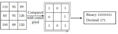
FIGURE 8.1 An example of LBP.

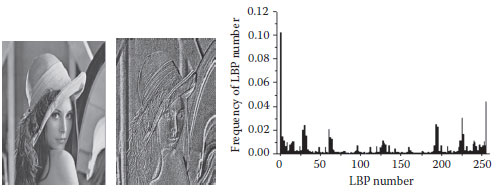
FIGURE 8.2 The texture spectrum and its histogram of image Lena processed by (8, 1) LBP operator.

${\text{LBP}}_p={\displaystyle \sum _{p=0}^{p-1}S\left(g_{\text{p}}-g_{\text{c}}\right)}\times 2^p$

(8.1)

where g_c denotes the gray level of the center pixel c in the P neighborhood, g_p denotes the gray level of the neighboring pixels p, and S(x) refers to the sign function defined as

$S\left(x\right)=\{\begin{array}{cc}1,& \text{if}x\ge 0\\ 0,& \text{otherwise}\end{array}$

(8.2)

Let I(M, N) be an image with a size of M × N, LBP_p(i, j) be the LBP pattern in the position of pixel I(i, j), h(k) be the histogram of texture spectrum, k = 0, 1, 2, …, 255, then

$h\left(k\right)=\frac{1}{M\times N}{\displaystyle \sum _{i=0}^{M-1}{\displaystyle \sum _{j=0}^{N-1}\text{δ}\left(i,j\right)}}$

(8.3)

where $\text{δ}\left(i,j\right)=\{\begin{array}{cc}1,& \text{LB}{\text{P}}_p\left(i,j\right)=k\\ 0,& \text{otherwise}\end{array}.$

Figure 8.2 shows the texture spectrum and its histogram of image Lena processed by an (8, 1) LBP operator.

8.2.2    EXTENSIONS OF ORIGINAL LBP OPERATORS

Similar to the original (P = 8, R = 1) LBP operator, we can extend the P and R to get different LBP operators of circle neighborhood by bilinear interpolation of Ahonen et al. (2004). Figure 8.3 presents some circle neighborhood. Compared with the original LBP operator, the extended LBP operators arrange their neighbor pixels along the circle, and describe the texture spectrums in different scales. The more the values of P and R, the more detailed the texture. We can choose different P and R according to our requirement.

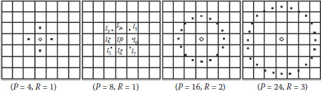
FIGURE 8.3 Some extended circle neighborhoods.

In order to lower the computational cost, Maenpaa (2008) provided another extended LBP operator called uniform LBP operator. By linking the head to tail, we can make the binary LBP pattern into a ring. In the ring, if times of spatial transitions from 0 to 1 or 1 to 0 are not more than 2, the LBP pattern can be a uniform LBP pattern. Experiments show that the uniform LBP pattern has a lower rate of recurrence, but describe most of the texture features. In the (P = 8, R = 1) LBP texture spectrum, uniform LBP pattern takes up 38%, but can present more than 90% texture pattern. Furthermore, it can reduce the quantity of texture features.

Let U be a uniform value of LBP pattern with (P, R), U can be computed as

$U\left({\text{LBP}}_{P,R}\right)={\displaystyle \sum _{i=0}^{P-1}\left|S\left(I_i-I_c\right)-S\left(I_{i+1}-I_c\right)\right|}$

(8.4)

where I_P = I₀. Any LBP pattern with U < 2 belongs to uniform pattern. In a circle neighborhood, there are P(P – 1) + 2 uniform patterns. Figure 8.4 shows some uniform LBP patterns and nonuniform LBP patterns of (P = 8, R = 1) neighborhood.

From the nature of texture, symmetric texture patterns should be regarded as a same pattern (see the example Figure 8.5), but they have different pattern values. By rotation of circle neighborhood, we can get a series of LBP pattern values and choose the minimum as the LBP pattern value of the circle neighborhood, as shown by Equation 8.5. Figure 8.6 gives an example of pattern rotation.

${\text{LBP}}_{P,R}^{ri}=\min \left\{\text{ROL}\left({\text{LBP}}_{P,R},i\right)\right\}$

(8.5)

Therefore, to achieve rotation invariance, a locally rotation invariant pattern can be defined as

${\text{LBP}}_{P,R}^{\text{riu}2}=\{\begin{array}{cc}{\displaystyle \sum _{i=0}^{P-1}S\left(I_i-I_c\right)}& U\le 2\\ P+1& \text{otherwise}\end{array}$

(8.6)

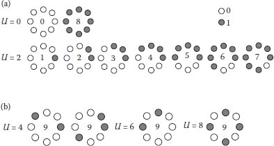
FIGURE 8.4 Some uniform LBP patterns and nonuniform LBP patterns of (P = 8, R = 1)neighborhoods. (a) Uniform LBP pattern and (b) nonuniform LBP pattern.

FIGURE 8.5 Examples of symmetric texture patterns.

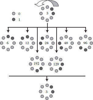
FIGURE 8.6 An example of pattern rotation.

where superscript “riu2” means rotation invariant uniform patterns with U ≤ 2. The mapping from LBP_P,_R to ${\text{LBP}}_{P,R}^{\text{riu2}}$ which has P + 2 distinct output values, can be implemented with a lookup table. More detailed information about the LBP operators and their applications can be referred to Ahonen et al. (2004) and Maenpaa (2008).

8.2.3    OTHER LBP OPERATORS

The LBP operators discussed above ignore the gray-level changes of pixels and illumination adaptability. In Zhang and Jin (2009), we improved the LBP operator by considering the magnitude of gray-level differences, which is important in texture description. It is noted that the improved LBP intends to concentrate on the visually most important texture pattern parts of images and disregard the unimportant details. The improved LBP operator introduced a parameter α to control the difference between neighboring pixels. If the difference between two pixels does not reach an extent controlled by α, it regards the two pixels as same. The improved LBP operator is defined as

${\text{LBP}}_p^{\text{α}}={\displaystyle \sum _{p=0}^{P-1}S\left(\frac{g_{\text{p}}-g_c}{g_c}-\text{α}\right)\times 2^p}$

(8.7)

The improved LBP operator is based on the features of video frames captured by the two-phase flow monitoring system and ignores the nonsignificant details, so that it can extract the most important texture patterns. If we change the sign function S(x) as:

$S_{\uparrow }\left(x\right)=\{\begin{array}{cc}1,& x>0\\ 0,& x\le 0\end{array}$

(8.8)

$S_{\downarrow }\left(x\right)=\{\begin{array}{cc}0,& x>0\\ 1,& x\le 0\end{array}$

(8.9)

we can obtain two LBP patterns, one of which (noted as LBP_↑) describes the distribution of pixels with gray levels larger than the center pixel, and the other (noted as LBP_↓) describes the distribution of pixels with gray levels lower than the center one. When reflecting on LBP texture spectrum, LBP_↑ captures the bright part of texture map, and LBP_↓ captures the dark part of texture map, they are compensatory with each other. The improved LBP operator has been applied in the gas-liquid two-phase flow regimes analysis and excellent results have been obtained. Similar to the improved LBP operator in thought, Tan and Triggs (2010) provided an enhanced LBP operator named LTP for face recognition and got satisfactory results.

Zhenhua et al. (2010) presented a completed modeling of the LBP operator (named by The Completed LBP) for texture classification. A local region or a neighborhood is represented by its center pixel and a local difference sign-magnitude transform. It decomposes the image local differences into two complementary components: the signs and the magnitudes, and obtains two LBP patterns. In fact, they performed another LBP operation on the magnitude and obtained another LBP pattern, besides sign LBP pattern. This completed LBP has been successfully used in the texture pattern recognition.

8.3    SPATIAL WATERMARKING BASED ON LBP OPERATORS

8.3.1    DEFINITIONS ON A (P, R) LOCAL REGION

Before presenting the proposed watermarking algorithms, we first provide some definitions. Let g_c denote the gray level of the center pixel c in the P neighborhood, and let g_p denote the gray level of the neighboring pixels p. For a (P, R) local region, we describe it as follows:

$g_{\text{p}}=\left\{g_i|i=0,\dots ,c,\dots ,P-1\right\}$

(8.10)

$m_{\text{p}}=\left\{m_i|m_i=\left|g_i-g_c\right|,i=0,\dots ,P-1\right\}$

(8.11)

$s_p=\left\{s_i|s_i=\text{sign}\left(g_i-g_c\right),i=0,\dots ,P-1\right\}$

(8.12)

Note that Equation 8.12 uses the sign function, which is equivalent to Equation 8.2. In this way, we divide the local region into three parts (Zhenhua et al., 2010): g_p is a vector composed of P pixels in the R radius, m_p is a vector built by the magnitude obtained from the difference between the p pixels and the center pixel g_c, and s_p is a sign vector from the difference. Figure 8.7 shows an example of the three parts in a (P = 8, R = 1) local region.

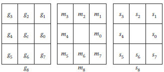
FIGURE 8.7 An example of a (8, 1) local region, as divided into three parts: g₈ is the pixel vector, m₈ is the magnitude vector, s₈ is the sign vector.

In order to embed watermarks, we define Boolean functions f(s_p) to be applied to the binary sign vector part s_p. Two types of Boolean functions are chosen for illustration purposes, which are defined as follows:

$f_{\oplus }\left(s_{\text{p}}\right)=s_0\oplus s_1\oplus \cdots \oplus s_{\text{P-1}}$

(8.13)

$f_{\#}\left(s_{\text{p}}\right)=\text{Bool}\left(\#1\left(s_{\text{p}}\right)-\#0\left(s_{\text{p}}\right)>N\right)$

(8.14)

In Equation 8.13, ⊕ is the exclusive OR (XOR) operator. Obviously, f_⊕(s_p) ∈ {0, 1}. It satisfies the associative and commutative properties, so any circular bit shifted on s_p clockwise or counterclockwise does not change the function value. However, any one bit change in s_p from 0 to 1 or from 1 to 0 will reverse the function value.

In Equation 8.14, #1(s_p) means the number of pixels with value “1” in s_p, #0(s_p) is the number of "0" in s_p, N is an integer, and N ≤ P – 1. If #1(s_p) – # 0(s_p) > N, then f_#(s_p) returns 1; otherwise, it returns 0. Obviously, f_#(s_p) is immune to bit shift and rotation.

8.3.2    WATERMARK-EMBEDDING ALGORITHM

We embed the watermarks by changing the value of f(s_p) in a local region. The value of f(S_p) is changed by altering the bits in s_p. These changes are reflected by modification of pixels in the spatial local region. Different Boolean functions correspond to different algorithms.

For instance, we use Boolean function f_⊕(s_p). In a (P, R) neighborhood, we select a pixel with the minimal magnitude in m_pto alter for embedding the watermark, so that we affect the quality of the original image block to its least degree. In other words, we keep the value of f_⊕(s_p) consistent with the corresponding bit of watermarks without reducing the quality of the image block much.

The watermark embedding procedure can be summarized in the following two steps:

1.  The original image is divided into (P, R) non-overlapping local region blocks. The LBP pattern is computed to obtain m_p and s_p, and then obtain the value of f_⊕(s_p). Let w be one of bits in the watermarks and β be the watermarking intensity factor.

2.  For each (P, R) local neighborhood, if the value of f_⊕(s_p) is equal to the value of w, we do nothing to the pixels in the neighborhood. Otherwise, we modify one of the pixels by making the value of f_⊕(s_p) consistent with the corresponding w. That is,

Note that min( ) is the minimal function. If there are more than one minimum, we select any one of the minimums to determine the pixel to be changed. If a block’s pixels are all “0” or “1,” we will modify the center pixel based on the corresponding watermarking bit before embedding it to the block.

8.3.3    WATERMARK EXTRACTION ALGORITHM

The watermark extraction procedure in the proposed method becomes straightforward. We judge the value of f_⊕(s_p) in the watermarked image to extract the watermark w. That is

8.4    EXPERIMENTAL RESULTS AND ANALYSIS

We use the Lena image of size 256 × 256 to test the performance of the algorithms shown in Section 8.3. The watermark is a binary image of size 84 × 84. The neighborhood is (8, 1), which is a 3 × 3 local region. One local region embeds one bit of watermark. Therefore, the watermarking capacity is 1/9 of the original image size.

The notations are given below. W(i, j) denotes the original watermark binary image of size M × M, W^*(i, j) denotes the extracted watermarked binary image of size M × M, F(i, j) denotes the original image of size N × N to be watermarked, and F^*(i,j) denotes the watermarked image. We use PSNR (peak signal-to-noise ratio), EBR (error bit rate), and NC (normalized correlation), as shown in Equations 8.8, (8.9), and (8.10), respectively, to evaluate the performance.

The EBR is used to compute the rate of error bits on the whole watermark accurate bits. The NC is used to locate a pattern on the extracted watermark image that best matches the specified reference pattern from the original image base, see Kung et al. (2009). Evidently, NC measures the amount of altered information which is originally “1”, and we name it as white NC(WNC). In order to accurately calculate the effect of the attack, the amount of altered information which is originally “0” is also considered, and we name it as black NC (BNC). Note that the formula of BNC is the same as Equation 8.9 with all 1’s being changed to 0’s and vice versa. The PSNR is often used in engineering to measure the signal ratio between the maximum power and the power of corrupting noise. We use it to compare the original and the embedded images in the spatial domain.

$\text{EBR=}\frac{{\displaystyle {\sum }_{i=0}^{M-1}{\displaystyle {\sum }_{j=0}^{M-1}\left(W\left(i,j\right)\oplus W^{\ast }\left(i,j\right)\right)}}}{M\times M}$

(8.15)

$\text{NC}=\frac{{\displaystyle {\sum }_{i=1}^M{\displaystyle {\sum }_{j=1}^{M}W\left(i,j\right)}{W}^{*}\left(i,j\right)}}{{\displaystyle {\sum }_{i=1}^M{\displaystyle {\sum }_{j=1}^M\left[W{\left(i,j\right)}^2\right]}}}$

(8.16)

$PSNR=10{\text{log}}_{10}\left[\frac{{255}^2}{{\displaystyle {\sum }_{i=1}^N{\displaystyle {\sum }_{j=1}^N{[F(i,j)-F^{\ast }(i,j)]}^2/N^2}}}\right]$

(8.17)

By experiments, the proposed (8,1) LBP-based watermarking algorithm shows better transparency and robustness against some commonly used image-processing operations, such as additive noise, luminance variation, contrast adjustment, and color balance. Some examples of applying various operations on the watermarked image are shown in Figure 8.8, where Figure 8.8a is the original Lena image, Figure 8.8b is the original watermark, Figure 8.8c is the watermarked Lena by the proposed algorithm with PSNR 42.67 and intensity factor β = 0.08, and Figure 8.8d is the extracted watermark with WNC = 1 and BNC = 1.

From Figure 8.8e–z, all processes are carried out in Figure 8.8c. Figure 8.8e is the resulting image after adding 10% noise, and Figure 8.8f is the extracted watermark with EBR = 3.85%, WNC = 0.959, and BNC = 0.962. Figure 8.8g is the resulting image after adding 30% noise, and Figure 8.8h is the extracted watermark with EBR = 10.01%, WNC = 0.887, and BNC = 0.905. Figure 8.8i is the resulting image after logarithm transform of darkening, and Figure 8.8j is the extracted watermark with EBR = 5.33%, WNC = 0.948, and BNC = 0.946. Figure 8.8k is the resulting image after logarithm transform of brightening, and Figure 8.8l is the extracted watermark with EBR = 2.98%, WNC = 0.979, and BNC = 0.966. Figure 8.8m is the resulting image after contrast enhancement of +10%, and Figure 8.8n is the extracted watermark with EBR = 0.47%, WNC = 0.995, and BNC = 0.995. Figure 8.8 is the resulting image after contrast reduction of -50%, and Figure 8.8p is the extracted watermark with EBR = 14.24%, WNC = 0.875, and BNC = 0.851.

Figure 8.8q is the resulting image after coloring by Photoshop 7.0, and Figure 8.8r is the extracted watermark with EBR = 1.03%, WNC = 0.990, and BNC = 0.989. Figure. 8.8s is the resulting image after color saturation adjustment, and Figure 8.8 t is the extracted watermark with EBR = 5.75%, WNC = 0.946, and BNC = 0.940. Figure 8.8u is the resulting image after destroying some parts, and Figure 8.8v is the extracted watermark with EBR = 7.17%. Figure 8.8p is the resulting image after cut from the original image, and Figure 8.8x is the extracted watermark. Figure 8.8y is the resulting image after JPEG compression by Photoshop 7.0 with quality 12, and Figure 8.8z is the extracted watermark with EBR = 19.20%, WNC = 0.80, and BNC = 0.81. Figure 8.8A is the resulting image after JPEG compression with quality 11, and Figure 8.8B is the extracted watermark with EBR = 35.12%, WNC = 0.648, and BNC = 0.656.

By experiments, the proposed method shows better image tamper detection ability. Figure 8.9 provides two examples. In Figure 8.9a, the enclosed face area of the watermarked Lena image (see Figure 8.8c) is replaced by the original (unwatermarked) face area in Figure 8.8a. The extracted watermark in Figure 8.9b reveals the modification, and Figure 8.9c shows the corresponding location of the modification.

Another example is the automobile license plate number forgery. Figure 8.9d shows an original license plate image, and Figure 8.9e is the watermarked image. Figure 8.9f is the tampered image by using the digit “2” to replace the character “M” in the license plate of Figure 8.9e. Figure 8.9g shows the result of tamper detection and location.

Figures 8.10, 8.11, 8.12, 8.13, 8.14 show some validation results. From Figure 8.10, as the intensity factor increases, the PSNR declines slowly, but maintains satisfactory values. When β reaches 0.3, the PSNR is still above 30, which demonstrates that the proposed method keeps good image quality. (Figure 8.11) shows its better power against noise. When adding noise is 50%, the watermarked image is nearly destroyed, but the EBR is only about 16%. It shows that the proposed method is very robust to noise. (Figure 8.12) embodies its good robustness against luminance modification. Luminance does not have much effect on LBP operators, which is shown in (Figure 8.12). The best characteristic of the proposed method is its anticontrast adjustment shown in (Figure 8.13), where the EBR keeps very low values especially when contrast adjustment increases from 0 to 10. When contrast increases to 50% or decreases to -50%, the EBR are below 15%. (Figure 8.14) demonstrates that it is only robust against slight JPEG compression. When compression keeps better quality, the method has EBR of <20%. However, the proposed method is fragile to medium filter, image blurring, pixel interpolation, and other operations on a window neighborhood.

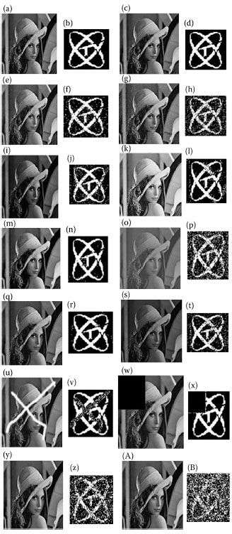
FIGURE 8.8 Examples of applying some image-processing operations on the watermarkedimage. (a) The original Lena image, (b) the original watermark, (c) the watermarked Lena bythe proposed algorithm with β = 0.08, (e)−(z): results by image-processing operations carriedout on (c). See context for more explanation. (A): is the resulting image after JPEG compressionand (B): is the extracted watermark

FIGURE 8.9 Tamper detection and location examples. (a) Tampered image by replacingface area, (b) the extracted watermark showing the tampering area, (c) tamper location, (d) original license plate, (e) watermarked license plate, (f) tampered license plate, and(g) tamper detection and location.

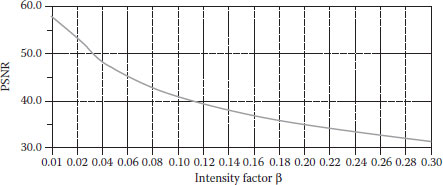
FIGURE 8.10 The relationship between PSNR and intensity factor.

FIGURE 8.11 The relationship between EBR and noise.

Although the function f_⊕(s_p) is invariant to rotation, the method achieves better results when the rotations are close to the multiples of 90°. It is because if any one of the bits in s_p changes from 0 to 1 or from 1 to 0, the value of f_⊕(s_p) will change to its inverse. To improve the robustness against rotation and compression, we use the function f_#(s_p) with N = 1 and watermark intensity factor β = 0.02. In the experiment, we modify the center pixel to satisfy the consistence between f_#(s_p) and the watermark bits. The watermark embedding algorithm is described as follows:

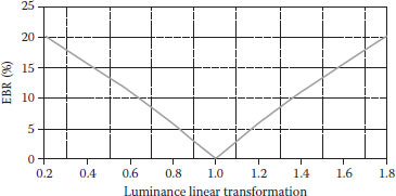
FIGURE 8.12 The relationship between EBR and luminance linear transformation.

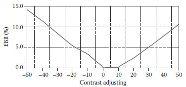
FIGURE 8.13 The relationship between EBR and contrast adjustment.

FIGURE 8.14 The relationship between EBR and JPEG compression.

if (w = 1 and f#(s_p) = 0) then do {g_c = g_c × (1 + β);

 Compute f_#(s_p);

 } while not f_#(s_p)

if (w = 0 and f_⊕(s_p) = 1) then do {g_c = g_c × (1 - β)

 Compute f_#(s_p);

 } while f_#(s_p)

By experiments, we observe that the function f_#(s_p) is more robust against additive noise, luminance change, contrast adjustment, JPEG compression, and rotation than the function f_⊕(s_p) is. Figures 8.15 and 8.16 show the results with respect to rotation and JPEG compression. From Figure 8.15, we see that the watermarked image rotates from 5°, 15°, 30°, 45°, 60°, 75°, 90°, the EBR is, respectively, 15.1, 11.8, 17.2, 25.9, 18.7, 16.8, and 0%. When the rotation angle is 45°, the result is the worst. Except for 90°, the angle 15° corresponds to the best result. From Figure 8.16, we see that the JPEG compression quality factors change from 12 to 6, the EBR is respectively 2.3, 5.9, 8.6, 12.4, 16.5, 25.1, and 18.2%. When the factor is 7, the EBR is the worst. With the decrease of the compression factors from 12 to 7, the EBR keeps an approximate lineal increase.

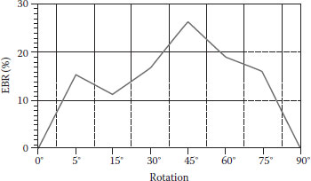
FIGURE 8.15 The relationship between EBR and rotation

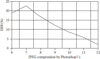
FIGURE 8.16 The relationship between EBR and JPEG compression.

8.5    MULTILEVEL WATERMARKING BASED ON LBP OPERATORS

We can extend the aforementioned watermarking algorithm to multilevel watermarking techniques to achieve higher-embedding capacity and better robustness. We firstly present a double-level watermarking algorithm and conduct analysis on its experimental results. Then, we extend it to a general framework for multilevel watermarking schemes.

8.5.1    DOUBLE-LEVEL WATERMARKING

We divide the neighborhood s_p into two parts: even and odd neighbors, denoted as s^e_p and s^e_p. We perform f⊕(s_p) on them and realize the embedding of two bits in the (P, R) neighborhood. In this way, the watermarking capacity is doubled. Figure 8.17 shows an example of the (8, 1) LBP pattern, which in fact is equivalent to two (4, 1) neighborhoods.

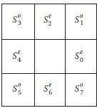
FIGURE 8.17 The s^e_pand s^e_pof (8, 1) LBP pattern. s^e_pdenotes even neighbors and s^e_pdenotes odd neighbors, p = 0…7.

An example of embedding two watermark images into the Lena image is shown inFigure 8.18, where Figure 8.18a is the original Lena image, Figure 8.18b and c are two watermark images denoted by W₁ and W₂, and Figure 8.18d is the watermarked image with PSNR = 36.5 and P = 0.08. Figures 8.18e and f are the two extracted watermarks from Figure 8.18d. Figure 8.18g is the resulting image after adding 10% noise, and Figure 8.18h and i are the extracted two watermarks with EBR = 1.96% and 2.47%, WNC = 0.980 and 0.966, BNC = 0.980 and 0.977, respectively. Figure 8.18j is the resulting image after adding noise 120%, and Figure 8.18k and l are the extracted two watermarks with EBR = 8.73% and 9.04%, WNC = 0.894 and 0.885, BNC = 0.919 and 0.916, respectively.

Figure 8.18m is the resulting image after luminance reduction of –50%, and Figure 8.18n and o are the extracted two watermarks with EBR = 10.23% and 7.74%, WNC = 0.916 and 0.949, BNC = 0.890 and 0.914, respectively. Figure 8.18p is the resulting image after luminance enhancement of +50%, and Figure 8.18q and r are the extracted two watermarks with EBR 10.08% and 7.55%, WNC = 0.923 and 0.946, BNC = 0.916 and 0.949, respectively. Figure 8.18s is the resulting image after contrast reduction of –50%, and Figure 8.18t and u are the extracted two watermarks with EBR = 10.07% and 8.86%, WNC = 0.918 and 0.942, BNC = 0.892 and 0.908, respectively. Figure 8.18v is the resulting image after JPEG compression with quality 12 by Photoshop 7.0, and Figure 8.18w and x are the extracted two watermarks with EBR = 12.47% and 8.42%, WNC = 0.882 and 0.925, BNC = 0.872 and 0.912, respectively.

Note that the embedding and extraction of two watermarks do not interfere with each other. Figures 8.19, 8.20, 8.21, 8.22 show the performance curves after applying some image-processing operations. We observe that the double-level watermarking technique performs better robustness than the single-level one. In Figure 8.19, when the double-level watermarked image is added by 50% noise, the extracted two watermarks are EBR 8.73 and 9.04%, but for single-level watermarking, EBR is 16.02%. InFigure 8.20, when the double-level watermarked image is compressed by JPEG with quality factor 12, the extracted two watermarks are EBR 12.47 and 8.42%, but for single-level watermark, EBR is 19.02%. InFigures 8.21 and 8.22, when the double-level watermarked image is applied by luminance or contrast adjustment, the extracted two watermarks are EBR 3–5% lower than the single-level one.

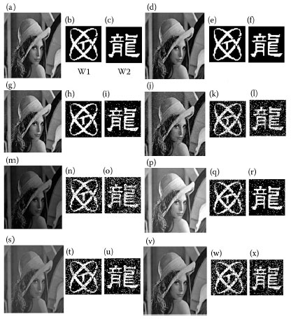
FIGURE 8.18 Examples of multilevel watermarking based on (8, 1) LBP pattern. (a) Theoriginal Lena image, (b, c) two watermark images W1 and W2, (d) the watermarked image, (e, f) the two extracted watermarks. (g, j, m, p, s, v) The resulting images by image-processing operations carried on (d). (h, i, k, l, n, o, q, r, t, u, w, x) The extracted watermarks from (g, j, m, p, s, v), respectively. See text for more explanation.

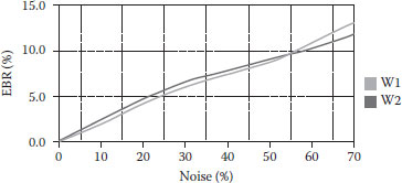
FIGURE 8.19 The relationship between EBR and Noise by double-level watermarking.

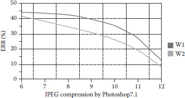
FIGURE 8.20 The relationship between EBR and JPEG compression by double-level watermarking.

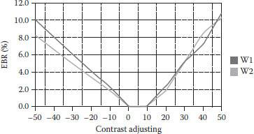
FIGURE 8.21 The relationship between EBR and contrast adjustment by double-level watermarking.

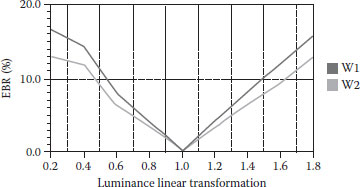
FIGURE 8.22 The relationship between EBR and luminance linear transformation by double-level watermarking..

8.5.2    EXTENSION TO MULTILEVEL WATERMARKING

Based on double-level watermarking, we can extend it to multilevel watermarking using variant (P, R) blocks to embed multiple watermarks. For example, four-level watermarking on the 5×5 neighborhood block is shown in Figure 8.23, which is divided into four parts: $s_i^1,s_i^2,s_j^3,s_j^4,i=0\cdots 3,j=0\cdots 7$. For $s_i^1$ and $s_i^2$, we use f_⊕(s_p) to embed watermarks, and for $s_j^3$ and $s_j^4$, we use f_#(s_p) on any one to embed watermarks and use f_#(s_p) on the other to embed watermarks. Therefore, we can embed four watermarks individually without mutual interference.

Let W_i, i = 0….3 be the four watermarks. In experiment, we firstly embed W₂and W₃, one of which is embedded by modifying the value of the center pixel (watermark factor β = 0.02), and the other by changing one of noncenter pixels (watermark factor β = 0.08). Then, we embed W₀ and W₁ based on Section 8.5.1.

Figure 8.24 shows some examples of multilevel watermarking.Figures 8.24a–d are the original images of size 256×256, and Figures 8.24e–h are the four watermark images of size 51 × 51. Figures 8.24i–l are the watermarked images with PSNR 36.11, 35.01, 38.24, and 36.7, respectively, and the four watermark images can be extracted exactly. Because the embedding procedures of the four watermarks do not affect each other, their performances are basically consistent with the results pro-vided previously in Sections 8.4 and 8.5.

Although the watermarked images achieve better PSNR, we can observe from Figure 8.24 that some pixels in the smooth white or black region of these images are changed obviously, just like additive noises. InFigure 8.24, we see that several points are protruding in smooth regions, while inFigure 8.24j, it is difficult to see those points. Therefore, the proposed multilevel watermarking technique is very suited for the images with more complicated textures.

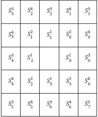
FIGURE 8.23 The four parts of sp in a 5 × 5 block. $s_i^1,s_i^2,s_j^3,s_j^4,i=0\cdots 3,j=0\cdots 7$ are used to embed the four watermarks, respectively.

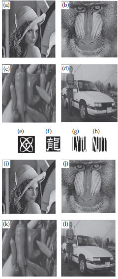
FIGURE 8.24 Multilevel watermarking examples. (a)-(d) are the four original images, (e)-(h) are the four watermark images, and (i)-(l) are the watermarked images extracted from(e)-(h), respectively. See text for further explanation.

The prooposed method can be similarly extended to other LBP operators with different (P, R). We can design many multilevel watermarking schemes by jointly using f_⊕(s_p)and f_#(s_p) or using other different functions. Furthermore, the proposed method can be applied to the improved and complete LBP operators (Zhang and Jin, 2009; Zhenhua et al., 2010) to embed multilevel watermarks.

8.6    CONCLUSIONS

In this chapter, a new semi-fragile spatial watermarking scheme based on the LBP operator is proposed, whose single-level and multilevel watermarking methods are described and analyzed. The proposed methods are robust against some commonly used image-processing operations, such as additive noise, luminance change, and contrast adjustment. At the same time, they maintain good fragility to some window operations, such as filtering and blurring, and have better sensitivity to image tampering. It can also achieve tamper detection and location.

For future research, we will focus on the comprehensive comparison of different watermarking schemes based on different LBP operators, their reversibility, and security. Also, we will conduct research on steganalysis based on LBP operators, as enlightened by Lafferty and Ahmed (2004).

REFERENCES

Ahonen, T., Hadid, A., and Pietikainen, M., Face recognition with local binary patterns, in Proc European Conf Computer Vision, Prague, Czech, pp. 469–481, 2004.

Bas, P., Bihan, N. L., and Chassery, J., Color watermarking using quaternion Fourier transform, in Proc ICASSP, Hong Kong, China, pp. 521–524, Jun. 2003.

Chen, B., and Wornell, G., Quantization index modulation methods for digital watermarking and information embedding of multimedia, J VLSI Signal Process, 27, 7–33, 2001.

Cox, I., Kilian, J., Leighton, F., and Shamoon, T., Secure spread spectrum watermarking for multimedia, IEEE Trans Image Process, 6(12), 1673–1687, 1997.

Cvejic, N., and Tujkovic, I., Increasing robustness of patchwork audio watermarking algorithm using attack characterization, in Proc. IEEE Int Symp Consumer Electronics, U.K., pp. 3–6, 2004.

Kaewkamnerd, N., and Rao, K. R., Wavelet based image adaptive watermarking scheme, Electron Lett, 36, 518–526, 2000.

Kung, C.-M., Chao, S.-T., Tu, Y.-C., Yan, Y.-H., and Kung, C.-H., A robust watermarking and image authentication scheme used for digital content application, J Multimed, 4(3), 112–119, 2009.

Lafferty, P., and Ahmed, F., Texture based steganalysis: Results for color images, mathematics of data/image coding, compression, and encryption VII, with applications, in Proc. of SPIE, 5561, 145–151, 2004.

Luo, L., Chen, Z., Chen, M., Zeng, X., and Xiong, Z.,, Reversible image watermarking using interpolation technique, IEEE Trans. Forensics Sec, 5(1), 187–196, 2010.

Maenpaa, T., The local binary pattern approach to texture analysis extensions and applications, 2003, website http://herkules.oulu.fi/isbn9514270762/. Last accessed Dec. 20, 2008.

Maenpaa, T., Pietikainen, M., and Ojala, T., Texture classification by multi-predicate local binary pattern operators, in Proc 15th Int Conf Pattern Recognition, Barcelona, Spain, pp., 951–954, 2000.

Ojala, T., Pietikainen, M., and Maenpaa, T., Multiresolution gray scale and rotation invariant texture analysis with local binary pattern, IEEE Trans Pattern Anal Mach Intell, 24(7), 971–987, 2002.

Pitas, I., A method for signature casting on digital images, in Proc IEEE Int Conf Image Process, III, 215–218, 1996.

Piva, A., Bartolini, F., Boccardi, L., Cappellin, V. De, Rosa, A. and Barni, M., Watermarking through color image bands decorrelation, in Proc IEEE Int Conf Multimedia Expo., New York, pp., 1283–1286, Jul. 30–Aug. 2, 2000.

Podilchuk, C., and Zeng, W., Image-adaptive watermarking using visual models, IEEE J Sel Areas Commun, 16(4), 525–539, 1998.

Reed, A., and Hannigan, B., Adaptive color watermarking, in Proc SPIE, 4675, 222, 2002.

Sachnev, V., Kim, H. J., Suresh, J. N. S., and Shi, Y. Q., Reversible watermarking algorithm using sorting and prediction, IEEE Trans Circuits Syst Video Technol, 19(7), 989–999, 2009.

Schyndel, R., Tirkel, A., and Osborne, C., A digital watermark, in Proc IEEE Int Conf Image Process, II, 86–90, 1994.

Shih, F. Y., Digital Watermarking and Steganography: Fundamentals and Techniques, CRC Press, Boca Raton, FL, 2008.

Shih, F. Y., and Wu, S., Combinational image watermarking in the spatial and frequency domains, Pattern Recognit, 36, 969–975, 2003.

Swanson, M., Zhu, B., and Tewfik, A., Transparent robust image watermarking, in Proc IEEE Int Conf Image Process, III, 211–214, 1996.

Tanaka, K., Nakamura, Y., and Matsui, K., Embedding secret information into a dithered multi-level image, in Proc IEEE ILCOM Int Conf, pp. 216–220, 1990.

Tan, X. and Triggs, B., Enhanced local texture feature sets for face recognition under difficult lighting conditions, IEEE Trans Image Process, 19(6), 1635–1650, 2010.

Tsui, T. K., Zhang, P., and Androutsos, D., Color image watermarking using multidimensional Fourier transforms, IEEE Trans Forensics Sec, 3(1), 16–28, 2008.

Wei, Z. and Ngan, K. N., Spatio-temporal just noticeable distortion profile for grey scale image/video in DCT domain, IEEE Trans Circuits Syst Video Technol, 19(3), 337–346, 2009.

Wu, H.-T. and Cheung, Y.-M., Reversible watermarking by modulation and security enhancement, IEEE Trans Instrum Meas, 59(1), 221–228, 2010.

Xia, X.-G., Boncelet, C. G., and Arce, G. R., A multiresolution watermark for digital images, in Proc IEEE Int Conf Image Process, I, 548–551, 1997.

Yang, Y., Sun, M., Yang, H., Li, C. T., and Xiao, R., A contrast-sensitive reversible visible image watermarking technique, IEEE Trans Circuits Syst Video Technol, 19(5), 656–667, 2009.

Yeo, I.-K. and Kim, H. J., Modified patchwork algorithm: A novel audio watermarking scheme, in Proc Int Conf Inf Technol: Coding Comput, pp. 237, 2001.

Zhang, W. Y. and Jin, N. D., Improved local binary pattern based gas-liquid two-phase flow regimes analysis, in Proc 6th Int Conf Fuzzy Syst Knowl Discov, August 2009.

Zhang, W. Y. and Shih, F. Y., Semi-fragile spatial watermarking based on local binary pattern operators, J Opt Commun, 284(16), 3904–3912, 2011.

Zhang, W. Y., Shih, F. Y., Jin, N., and Liu, Y., Recognition of gas-liquid two-phase flow patterns based on improved local binary pattern operator, Int J Multiph Flow, 36, 793–797, 2010.

Zhenhua, G., Zhang, L., and Zhang, D., A completed modeling of local binary pattern operator for texture classification, IEEE Trans Image Process, 19(6), 1657–1663, 2010.