
Chapter 9
Signal Processing
In graphics, we often deal with functions of a continuous variable: an image is the first example you have seen, but you will encounter many more as you continue your exploration of graphics. By their nature, continuous functions can’t be directly represented in a computer; we have to somehow represent them using a finite number of bits. One of the most useful approaches to representing continuous functions is to use samples of the function: just store the values of the function at many different points and reconstruct the values in between when and if they are needed.
You are by now familiar with the idea of representing an image using a two-dimensional grid of pixels—so you have already seen a sampled representation! Think of an image captured by a digital camera: the actual image of the scene that was formed by the camera’s lens is a continuous function of the position on the image plane, and the camera converted that function into a two-dimensional grid of samples. Mathematically, the camera converted a function of type ℝ2 → C (where C is the set of colors) to a two-dimensional array of color samples, or a function of type ℤ2 → C.
Another example of a sampled representation is a 2D digitizing tablet, such as the screen of a tablet computer or a separate pen tablet used by an artist. In this case, the original function is the motion of the stylus, which is a time-varying 2D position, or a function of type ℝ → ℝ2. The digitizer measures the position of the stylus at many points in time, resulting in a sequence of 2D coordinates, or a function of type ℤ → ℝ2. A motion capture system does exactly the same thing for a special marker attached to an actor’s body: it takes the 3D position of the marker over time (ℝ → ℝ3) and makes it into a series of instantaneous position measurements (ℤ → ℝ3).
Going up in dimension, a medical CT scanner, used to non-invasively examine the interior of a person’s body, measures density as a function of position inside the body. The output of the scanner is a 3D grid of density values: it converts the density of the body (ℝ3 → ℝ) to a 3D array of real numbers (ℤ3 → ℝ).
These examples seem different, but in fact they can all be handled using exactly the same mathematics. In all cases a function is being sampled at the points of a lattice in one or more dimensions, and in all cases we need to be able to reconstruct that original continuous function from the array of samples.
From the example of a 2D image, it may seem that the pixels are enough, and we never need to think about continuous functions again once the camera has discretized the image. But what if we want to make the image larger or smaller on the screen, particularly by non-integer scale factors? It turns out that the simplest algorithms to do this perform badly, introducing obvious visual artifacts known as aliasing. Explaining why aliasing happens and understanding how to prevent it require the mathematics of sampling theory. The resulting algorithms are rather simple, but the reasoning behind them, and the details of making them perform well, can be subtle.
Representing continuous functions in a computer is, of course, not unique to graphics; nor is the idea of sampling and reconstruction. Sampled representations are used in applications from digital audio to computational physics, and graphics is just one (and by no means the first) user of the related algorithms and mathematics. The fundamental facts about how to do sampling and reconstruction have been known in the field of communications since the 1920s and were stated in exactly the form we use them by the 1940s (Shannon & Weaver, 1964).
This chapter starts by summarizing sampling and reconstruction using the concrete one-dimensional example of digital audio. Then, we go on to present the basic mathematics and algorithms that underlie sampling and reconstruction in one and two dimensions. Finally, we go into the details of the frequency-domain viewpoint, which provides many insights into the behavior of these algorithms.
9.1 Digital Audio: Sampling in 1D
Although sampled representations had already been in use for years in telecommunications, the introduction of the compact disc in 1982, following the increased use of digital recording for audio in the previous decade, was the first highly visible consumer application of sampling.
In audio recording, a microphone converts sound, which exists as pressure waves in the air, into a time-varying voltage that amounts to a measurement of the changing air pressure at the point where the microphone is located. This electrical signal needs to be stored somehow so that it may be played back at a later time and sent to a loudspeaker that converts the voltage back into pressure waves by moving a diaphragm in synchronization with the voltage.
The digital approach to recording the audio signal (Figure 9.1) uses sampling: an analog-to-digital converter (A/D converter, or ADC) measures the voltage many thousand times per second, generating a stream of integers that can easily be stored on any number of media, say a disk on a computer in the recording studio, or transmitted to another location, say the memory in a portable audio player. At playback time, the data is read out at the appropriate rate and sent to a digital-to-analog converter (D/A converter, or DAC). The DAC produces a voltage according to the numbers it receives, and, provided we take enough samples to fairly represent the variation in voltage, the resulting electrical signal is, for all practical purposes, identical to the input.

It turns out that the number of samples per second required to end up with a good reproduction depends on how high-pitched the sounds are that we are trying to record. A sample rate that works fine for reproducing a string bass or a kick drum produces bizarre-sounding results if we try to record a piccolo or a cymbal; but those sounds are reproduced just fine with a higher sample rate. To avoid these undersampling artifacts the digital audio recorder filters the input to the ADC to remove high frequencies that can cause problems.
Another kind of problem arises on the output side. The DAC produces a voltage that changes whenever a new sample comes in, but stays constant until the next sample, producing a stair-step shaped graph. These stair-steps act like noise, adding a high-frequency, signal-dependent buzzing sound. To remove this reconstruction artifact, the digital audio player filters the output from the DAC to smooth out the waveform.
9.1.1 Sampling Artifacts and Aliasing
The digital audio recording chain can serve as a concrete model for the sampling and reconstruction processes that happen in graphics. The same kind of under-sampling and reconstruction artifacts also happen with images or other sampled signals in graphics, and the solution is the same: filtering before sampling and filtering again during reconstruction.
A concrete example of the kind of artifacts that can arise from too-low sample frequencies is shown in Figure 9.2. Here we are sampling a simple sine wave using two different sample frequencies: 10.8 samples per cycle on the top and 1.2 samples per cycle on the bottom. The higher rate produces a set of samples that obviously capture the signal well, but the samples resulting from the lower sample rate are indistinguishable from samples of a low-frequency sine wave—in fact, faced with this set of samples the low-frequency sinusoid seems the more likely interpretation.

A sine wave (blue curve) sampled at two different rates. Top: at a high sample rate, the resulting samples (black dots) represent the signal well. Bottom: a lower sample rate produces an ambiguous result: the samples are exactly the same as would result from sampling a wave of much lower frequency (dashed curve).
Once the sampling has been done, it is impossible to know which of the two signals—the fast or the slow sine wave—was the original, and therefore there is no single method that can properly reconstruct the signal in both cases. Because the high-frequency signal is “pretending to be” a low-frequency signal, this phenomenon is known as aliasing.
Aliasing shows up whenever flaws in sampling and reconstruction lead to artifacts at surprising frequencies. In audio, aliasing takes the form of odd-sounding extra tones—a bell ringing at 10KHz, after being sampled at 8KHz, turns into a 6KHz tone. In images, aliasing often takes the form of moireé patterns that result from the interaction of the sample grid with regular features in an image, for instance the window blinds in Figure 9.34.
Another example of aliasing in a synthetic image is the familiar stair-stepping on straight lines that are rendered with only black and white pixels (Figure 9.34). This is an example of small-scale features (the sharp edges of the lines) creating artifacts at a different scale (for shallow-slope lines the stair steps are very long).
The basic issues of sampling and reconstruction can be understood simply based on features being too small or too large, but some more quantitative questions are harder to answer:
- What sample rate is high enough to ensure good results?
- What kinds of filters are appropriate for sampling and reconstruction?
- What degree of smoothing is required to avoid aliasing?
Solid answers to these questions will have to wait until we have developed the theory fully in Section 9.5
9.2 Convolution
Before we discuss algorithms for sampling and reconstruction, we’ll first examine the mathematical concept on which they are based—convolution. Convolution is a simple mathematical concept that underlies the algorithms that are used for sampling, filtering, and reconstruction. It also is the basis of how we will analyze these algorithms later in the chapter.
Convolution is an operation on functions: it takes two functions and combines them to produce a new function. In this book, the convolution operator is denoted by a star: the result of applying convolution to the functions f and g is f ★ g. We say that f is convolved with g, and f ★ g is the convolution of f and g.
Convolution can be applied either to continuous functions (functions f(x) that are defined for any real argument x) or to discrete sequences (functions a[i] that are defined only for integer arguments i). It can also be applied to functions defined on one-dimensional, two-dimensional, or higher-dimensional domains (that is, functions of one, two, or more arguments). We will start with the discrete, one-dimensional case first, then continue to continuous functions and two- and three-dimensional functions.
For convenience in the definitions, we generally assume that the functions’ domains go on forever, though of course in practice they will have to stop somewhere, and we have to handle the endpoints in a special way.
9.2.1 Moving Averages
To get a basic picture of convolution, consider the example of smoothing a 1D function using a moving average (Figure 9.3). To get a smoothed value at any point, we compute the average of the function over a range extending a distance r in each direction. The distance r, called the radius of the smoothing operation, is a parameter that controls how much smoothing happens.

We can state this idea mathematically for discrete or continuous functions. If we’re smoothing a continuous function g(x), averaging means integrating g over an interval and then dividing by the length of the interval:
On the other hand, if we’re smoothing a discrete function a[i], averaging means summing a for a range of indices and dividing by the number of values:
In each case, the normalization constant is chosen so that if we smooth a constant function the result will be the same function.
This idea of a moving average is the essence of convolution; the only difference is that in convolution the moving average is a weighted average.
9.2.2 Discrete Convolution
We will start with the most concrete case of convolution: convolving a discrete sequence a[i] with another discrete sequence b[i]. The result is a discrete sequence (a ★ b)[i]. The process is just like smoothing a with a moving average, but this time instead of equally weighting all samples within a distance r, we use a second sequence b to give a weight to each sample (Figure 9.4). The value b[i – j] gives the weight for the sample at position j, which is at a distance i – j from the index i where we are evaluating the convolution. Here is the definition of (a ★ b), expressed as a formula:

Computing one value in the discrete convolution of a sequence a with a filter b that has support five samples wide. Each sample in a ★ b is an average of nearby samples in a, weighted by the values of b.
By omitting bounds on j, we indicate that this sum runs over all integers (that is, from −∞ to +∞). Figure 9.4 illustrates how one output sample is computed, using the example of [..., 0, 1, 4, 6, 4, 1, 0,...] —that is, , , etc.
In graphics, one of the two functions will usually have finite support (as does the example in Figure 9.4), which means that it is nonzero only over a finite interval of argument values. If we assume that b has finite support, there is some radius r such that b[k] = 0 whenever |k| > r. In that case, we can write the sum above as
and we can express the definition in code as
function convolve(sequence a, filter b, int i)
s = 0
r = b.radius
for j = i - r to i + r do
s = s + a[j]b[i - j]
return s
Convolution Filters
Convolution is important because we can use it to perform filtering. Looking back at our first example of filtering, the moving average, we can now reinterpret that smoothing operation as convolution with a particular sequence. When we compute an average over some limited range of indices, that is the same as weighting the points in the range all identically and weighting the rest of the points with zeros. This kind of filter, which has a constant value over the interval where it is nonzero, is known as a box filter (because it looks like a rectangle if you draw its graph—see Figure 9.5). For a box filter of radius r the weight is 1/(2r + 1):

If you substitute this filter into Equation (9.2), you will find that it reduces to the moving average in Equation (9.1).
As in this example, convolution filters are usually designed so that they sum to 1. That way, they don’t affect the overall level of the signal.
Example (Convolution of a box and a step).
For a simple example of filtering, let the signal be the step function
and the filter be the five-point box filter centered at zero,
What is the result of convolving a and b? At a particular index i, as shown in Figure 9.6, the result is the average of the step function over the range from i – 2 to i + 2. If i < −2, we are averaging all zeros and the result is zero. If i ≥ 2, we are averaging all ones and the result is one. In between there are i + 3 ones, resulting in the value . The output is a linear ramp that goes from 0 to 1 over five samples: [..., 0, 0, 1, 2, 3, 4, 5, 5,...].

Properties of Convolution
The way we’ve written it so far, convolution seems like an asymmetric operation: a is the sequence we’re smoothing, and b provides the weights. But one of the nice properties of convolution is that it actually doesn’ t make any difference which is which: the filter and the signal are interchangeable. To see this, just rethink the sum in Equation (9.2) with the indices counting from the origin of the filter b, rather than from the origin of a. That is, we replace j with i – k. The result of this change of variable is
This is exactly the same as Equation (9.2) but with a acting as the filter and b acting as the signal. So for any sequences a and b, (a ★ b) = (b ★ a), and we say that convolution is a commutative operation.1
More generally, convolution is a “multiplication-like” operation. Like multiplication or addition of numbers or functions, neither the order of the arguments nor the placement of parentheses affects the result. Also, convolution relates to addition in the same way that multiplication does. To be precise, convolution is commutative and associative, and it is distributive over addition.
These properties are very natural if we think of convolution as being like multiplication, and they are very handy to know about because they can help us save work by simplifying convolutions before we actually compute them. For instance, suppose we want to take a sequence a and convolve it with three filters, b1, b2, and b3—that is, we want ((a★b1)★b2)★b3. If the sequence is long and he filters are short (that is, they have small radii), it is much faster to first convolve the three filters together (computing b1 ★ b2★b3) and finally to convolve the result with the signal, computing a ★ (b1 ★ b2 ★ b3), which we know from associativity gives the same result.
A very simple filter serves as an identity for discrete convolution: it is the discrete filter of radius zero, or the sequence d[i] = ..., 0, 0,1, 0,0,... (Figure 9.7). If we convolve d with a signal a, there will be only one nonzero term in the sum:

So clearly, convolving a with d just gives back a again. The sequence d is known as the discrete impluse. It is occasionally useful in expressing a filter: for instance, the process of smoothing a signal a with a filter b and then subtracting that from the original could be expressed as a single convolution with the filter d − b:
9.2.3 Convolution as a Sum of Shifted Filters
There is a second, entirely equivalent, way of interpreting Equation (9.2). Looking at the samples of a★b one at a time leads to the weighted-average interpretation that we have already seen. But if we omit the [i], we can instead think of the sum as adding together entire sequences. One piece of notation is required to make this work: if b is a sequence, then the same sequence shifted to the right by j places is called b→j (Figure 9.8):

Then, we can write Equation (9.2) as a statement about the whole sequence (a★b) rather than element-by-element:
Looking at it this way, the convolution is a sum of shifted copies of b, weighted by the entries of a (Figure 9.9). Because of commutativity, we can pick either a or b as the filter; if we choose b, then we are adding up one copy of the filter for every sample in the input.

9.2.4 Convolution with Continuous Functions
While it is true that discrete sequences are what we actually work with in a computer program, these sampled sequences are supposed to represent continuous functions, and often we need to reason mathematically about the continuous functions in order to figure out what to do. For this reason, it is useful to define convolution between continuous functions and also between continuous and discrete functions.
The convolution of two continuous functions is the obvious generalization of Equation (9.2), with an integral replacing the sum:
One way of interpreting this definition is that the convolution of f and g, evaluated at the argument x, is the area under the curve of the product of the two functions after we shift g so that g(0) lines up with f(t). Just like in the discrete case, the convolution is a moving average, with the filter providing the weights for the average (see Figure 9.10).

Like discrete convolution, convolution of continuous functions is commutative and associative, and it is distributive over addition. Also as with the discrete case, the continuous convolution can be seen as a sum of copies of the filter rather than the computation of weighted averages. Except, in this case, there are infinitely many copies of the filter g:
Example (Convolution of two box functions).
Let f be a box function:
Then what is f ★ f? The definition (Equation 9.3) gives
Figure 9.11 shows the two cases of this integral. The two boxes might have zero overlap, which happens when x ≤ −1 or x ≥ 1 ; in this case the result is zero. When −1 < x < 1, the overlap depends on the separation between the two boxes, which is |x|; the result is 1 −|x|. So

This function, known as the tent function, is another common filter (see Section 9.3.1).
The Dirac Delta Function
In discrete convolution, we saw that the discrete impulse d acted as an identity: d ★ a = a. In the continuous case, there is also an identity function, called the Dirac impulse or Dirac delta function, denoted δ(x).
Intuitively, the delta function is a very narrow, very tall spike that has infinitesimal width but still has area equal to 1 (Figure 9.12). The key defining property of the delta function is that multiplying it by a function selects out the value exactly at zero:

The delta function does not have a well-defined value at 0 (you can think of its value loosely as +∞), but it does have the value δ(x) = 0 for all x ≠ 0.
From this property of selecting out single values, it follows that the delta function is the identity for continuous convolution (Figure 9.13), because convolving δ with any function f yields

So δ ★ f = f (and because of commutativity f ★ δ = f also).
9.2.5 Discrete-Continuous Convolution
There are two ways to connect the discrete and continuous worlds. One is sampling: we convert a continuous function into a discrete one by writing down the function’s value at all integer arguments and forgetting about the rest. Given a continuous function f(x), we can sample it to convert to a discrete sequence a[i]:
Going the other way, from a discrete function, or sequence, to a continuous function, is called reconstruction. This is accomplished using yet another form of convolution, the discrete-continuous form. In this case, we are filtering a discrete sequence a[i] with a continuous filter f(x):
The value of the reconstructed function a★f at x is a weighted sum of the samples a[i] for values of i near x (Figure 9.14). The weights come from the filter f, which is evaluated at a set of points spaced one unit apart. For example, if x = 5.3 and f has radius 2, f is evaluated at 1.3, 0.3, −0.7, and −1.7. Note that for discrete-continuous convolution we generally write the sequence first and the filter second, so that the sum is over integers.

As with discrete convolution, we can put bounds on the sum if we know the filter’s radius, r, eliminating all points where the difference between x and i is at least r:
Note, that if a point falls exactly at distance r from x (i.e., if x − r turns out to be an integer), it will be left out of the sum. This is in contrast to the discrete case, where we included the point at i − r.
Expressed in code, this is:
function reconstruct(sequence a, filter f, real x)
s = 0
r = f.radius
for i = ⌈x − r⌉ to ⌊x + r⌋ do
s = s + a[i]f(x – i)
return s
As with the other forms of convolution, discrete-continuous convolution may be seen as summing shifted copies of the filter (Figure 9.15):

Reconstruction (discrete-continuous convolution) as a sum of shifted copies of the filter.
Discrete-continuous convolution is closely related to splines. For uniform splines (a uniform B-spline, for instance), the parameterized curve for the spline is exactly the convolution of the spline’s basis function with the control point sequence (see Section 15.6.2).
9.2.6 Convolution in More Than One Dimension
So far, everything we have said about sampling and reconstruction has been one-dimensional: there has been a single variable x or a single sequence index i. Many of the important applications of sampling and reconstruction in graphics, though, are applied to two-dimensional functions—in particular, to 2D images. Fortunately, the generalization of sampling algorithms and theory from 1D to 2D, 3D, and beyond is conceptually very simple.
Beginning with the definition of discrete convolution, we can generalize it to two dimensions by making the sum into a double sum:
If b is a finitely supported filter of radius r (that is, it has (2r + 1)2 values), then we can write this sum with bounds (Figure 9.16):

The weights for the nine input samples that contribute to the discrete convolution at point (i, j) with a filter b of radius 1.
function convolve2d(sequence2d a, filter2d b, int i, int j)
s = 0
r = b.radius
for i' = i − r to i + r do
for j' = j – r to j + r do
s = s + a[i'][j']b[i – i'][j – j']
return s
This definition can be interpreted in the same way as in the 1D case: each output sample is a weighted average of an area in the input, using the 2D filter as a “mask” to determine the weight of each sample in the average.
Continuing the generalization, we can write continuous-continuous (Figure 9.17) and discrete-continuous (Figure 9.18) convolutions in 2D as well:

The weight for an infinitesimal area in the input signal resulting from continuous convolution at (x, y).

The weights for the 16 input samples that contribute to the discrete-continuous convolution at point (x, y) for a reconstruction filter of radius 2.
In each case, the result at a particular point is a weighted average of the input near that point. For the continuous-continuous case, it is a weighted integral over a region centered at that point, and in the discrete-continuous case it is a weighted average of all the samples that fall near the point.
Once we have gone from 1D to 2D, it should be fairly clear how to generalize further to 3D or even to higher dimensions.
9.3 Convolution Filters
Now that we have the machinery of convolution, let’s examine some of the particular filters commonly used in graphics.
Each of the following filters has a natural radius, which is the default size to be used for sampling or reconstruction when samples are spaced one unit apart. In this section filters are defined at this natural size: for instance, the box filter has a natural radius of , and the cubic filters have a natural radius of 2. We also arrange for each filter to integrate to 1: , as required for sampling and reconstruction without changing a signal’s average value.
As we will see in Section 9.4.3, some applications require filters of different sizes, which can be obtained by scaling the basic filter. For a filter f(x), we can define a version of scale s:
The filter is stretched horizontally by a factor of s, and then squashed vertically by a factor so that its area is unchanged. A filter that has a natural radius of r and is used at scale s has a radius of support sr (see Figure 9.20 below).
9.3.1 A Gallery of Convolution Filters
The Box Filter
The box filter (Figure 9.19) is a piecewise constant function whose integral is equal to one. As a discrete filter, it can be written as

Note that for symmetry we include both endpoints.
As a continuous filter, we write
In this case, we exclude one endpoint, which makes the box of radius 0.5 usable as a reconstruction filter. It is because the box filter is discontinuous that these boundary cases are important, and so for this particular filter we need to pay attention to them. We write just fbox for the natural radius of .
The Tent Filter
The tent, or linear filter (Figure 9.20), is a continuous, piecewise linear function:

Its natural radius is 1. For filters, such as this one, that are at least C0(that is, there are no sudden jumps in the value, as there are with the box), we no longer need to separate the definitions of the discrete and continuous filters: the discrete filter is just the continuous filter sampled at the integers.
The Gaussian Filter
The Gaussian function (Figure 9.21), also known as the normal distribution, is an important filter theoretically and practically. We’ll see more of its special properties as the chapter goes on:

The parameter σ is called the standard deviation. The Gaussian makes a good sampling filter because it is very smooth; we’ll make this statement more precise later in the chapter.
The Gaussian filter does not have any particular natural radius; it is a useful sampling filter for a range of σ. The Gaussian also does not have a finite radius of support, although because of the exponential decay, its values rapidly become small enough to ignore. When necessary, then, we can trim the tails from the function by setting it to zero outside some radius r, resulting in a trimmed Gaussian. This means that the filter’s width and natural radius can vary depending on the application, and a trimmed Gaussian scaled by s is the same as an unscaled trimmed Gaussian with standard deviation sσ and radius sr. The best way to handle this in practice is to let σ and r be set as properties of the filter, fixed when the filter is specified, and then scale the filter just like any other when it is applied.
The B-Spline Cubic Filter
Many filters are defined as piecewise polynomials, and cubic filters with four pieces (natural radius of 2) are often used as reconstruction filters. One such filter is known as the B-spline filter (Figure 9.22) because of its origins as a blending function for spline curves (see Chapter 15):

Among piecewise cubics, the B-spline is special because it has continuous first and second derivatives—that is, it is C2. A more concise way of defining this filter is fB = fbox ★ fbox ★ fbox ★ fbox; proving that the longer form above is equivalent is a nice exercise in convolution (see Exercise 3).
The Catmull-Rom Cubic Filter
Another piecewise cubic filter named for a spline, the Catmull-Rom filter (Figure 9.23), has the value zero at x = −2, −1,1, and 2, which means it will interpolate the samples when used as a reconstruction filter (Section 9.3.2):

The Mitchell-Netravali Cubic Filter
For the all-important application of resampling images, Mitchell and Netravali (Mitchell & Netravali, 1988) made a study of cubic filters and recommended one partway between the previous two filters as the best all-around choice (Figure 9.24). It is simply a weighted combination of the previous two filters:

9.3.2 Properties of Filters
Filters have some traditional terminology that goes with them, which we use to describe the filters and compare them to one another.
The impulse response of a filter is just another name for the function: it is the response of the filter to a signal that just contains an impluse (and recall that convolving with an impulse just gives back the filter).
A continuous filter is interpolating if, when it is used to reconstruct a continuous function from a discrete sequence, the resulting function takes on exactly the values of the samples at the sample points— that is, it “connects the dots” rather than producing a function that only goes near the dots. Interpolating filters are exactly those filters f for which f(0) = 1 and f(i) = 0 for all nonzero integers i(Figure 9.25).

An interpolating filter reconstructs the sample points exactly because it has the value zero at all nonzero integer offsets from the center.
A filter that takes on negative values has ringing or overshoot: it will produce extra oscillations in the value around sharp changes in the value of the function being filtered.
For instance, the Catmull-Rom filter has negative lobes on either side, and if you filter a step function with it, it will exaggerate the step a bit, resulting in function values that undershoot 0 and overshoot 1 (Figure 9.26).

A filter with negative lobes will always produce some overshoot when filtering or reconstructing a sharp discontinuity.
A continuous filter is ripple free if, when used as a reconstruction filter, it will reconstruct a constant sequence as a constant function (Figure 9.27). This is equivalent to the requirement that the filter sum to one on any integer-spaced grid:

The tent filter of radius 1 is a ripple-free reconstruction filter; the Gaussian filter with standard deviation 1/2 is not.
All the filters in Section 9.3.1 are ripple free at their natural radii, except the Gaussian, but none of them are necessarily ripple free when they are used at a noninteger scale. If it is necessary to eliminate ripple in discrete-continuous convolution, it is easy to do so: divide each computed sample by the sum of the weights used to compute it:
This expression can still be interpreted as convolution between a and a filter (see Exercise 6).
A continuous filter has a degree of continuity, which is the highest-order derivative that is defined everywhere. A filter, like the box filter, that has sudden jumps in its value is not continuous at all. A filter that is continuous but has sharp corners (discontinuities in the first derivative), such as the tent filter, has order of continuity zero, and we say it is C0. A filter that has a continuous derivative (no sharp corners), such as the piecewise cubic filters in the previous section, is C1; if its second derivative is also continuous, as is true of the B-spline filter, it is C2. The order of continuity of a filter is particularly important for a reconstruction filter because the reconstructed function inherits the continuity of the filter.
Separable Filters
So far we have only discussed filters for 1D convolution, but for images and other multidimensional signals we need filters too. In general, any 2D function could be a 2D filter, and occasionally it is useful to define them this way. But, in most cases, we can build suitable 2D (or higher-dimensional) filters from the 1D filters we have already seen.
The most useful way of doing this is by using a separable filter. The value of a separable filter f2(x, y) at a particular x and y is simply the product of f1 (the 1D filter) evaluated at x and at y:
Similarly, for discrete filters,
Any horizontal or vertical slice through f2 is a scaled copy of f1. The integral of f2 is the square of the integral of f1, so in particular if f1 is normalized, then so is f2.
Example (The separable tent filter).
If we choose the tent function for f1, the resulting piecewise bilinear function (Figure 9.28) is

The profiles along the coordinate axes are tent functions, but the profiles along the diagonals are quadratics (for instance, along the line x = y in the positive quadrant, we see the quadratic function (1 – x)2).
Example (The 2D Gaussian filter).
If we choose the Gaussian function for f1, the resulting 2D function (Figure 9.29) is

Notice that this is (up to a scale factor) the same function we would get if we revolved the 1D Gaussian around the origin to produce a circularly symmetric function. The property of being both circularly symmetric and separable at the same time is unique to the Gaussian function. The profiles along the coordinate axes are Gaussians, but so are the profiles along any direction at any offset from the center.
The key advantage of separable filters over other 2D filters has to do with efficiency in implementation. Let’s substitute the definition of a2 into the definition of discrete convolution:
Note that b1[i – i'] does not depend on j' and can be factored out of the inner sum:
Let’s abbreviate the inner sum as S[i']:
With the equation in this form, we can first compute and store S[i'] for each value of i', and then compute the outer sum using these stored values. At first glance this does not seem remarkable, since we still had to do work proportional to (2r + 1)2 to compute all the inner sums. However, it’s quite different if we want to compute the value at many points [i, j].
Suppose we need to compute a ★ b2 at [2, 2] and [3, 2], and b1 has a radius of 2. Examining Equation 9.5, we can see that we will need S[0],..., S[4] to compute the result at [2, 2], and we will need S[1],..., S[5] to compute the result at [3, 2]. So, in the separable formulation, we can just compute all six values of S and share S[1],..., S[4] (Figure 9.30).

Computing two output points using separate 2D arrays of 25 samples (above) vs. filtering once along the columns, then using separate 1D arrays of five samples (below).
This savings has great significance for large filters. Filtering an image with a filter of radius r in the general case requires computation of (2r + 1)2 products per pixel, while filtering the image with a separable filter of the same size requires 2(2r + 1) products (at the expense of some intermediate storage). This change in asymptotic complexity from O(r2) to O(r) enables the use of much larger filters.
function filterImage(image I, filter b)
r = b.radius
nx = I.width
ny = I.height
allocate storage array S[0 ... nx – 1]
allocate image Iout [r ... nx – r – 1, r ... ny – r – 1]
initialize S and Iout to all zero
for j = r to ny – r – 1 do
for i' = 0 to nx – 1 do
S[i'] = 0
for j' = j – r to j + r do
S[i'] = S[i'] + I[i', j'] b[j – j']
for i = r to nx – r – 1 do
for i' = i − r to i + r do
Iout[i, j] = Iout[i, j] + S[i']b[i – i']
return Iout
For simplicity, this function avoids all questions of boundaries by trimming r pixels off all four sides of the output image. In practice there are various ways to handle the boundaries; see Section 9.4.3.
9.4 Signal Processing for Images
We have discussed sampling, filtering, and reconstruction in the abstract so far, using mostly 1D signals for examples. But as we observed at the beginning of the chapter, the most important and most common application of signal processing in graphics is for sampled images. Let us look carefully at how all this applies to images.
9.4.1 Image Filtering Using Discrete Filters
Perhaps the simplest application of convolution is processing images using discrete convolution. Some of the most widely used features of image manipulation programs are simple convolution filters. Blurring of images can be achieved by convolving with many common lowpass filters, ranging from the box to the Gaussian (Figure 9.31). A Gaussian filter creates a very smooth-looking blur and is commonly used for this purpose.
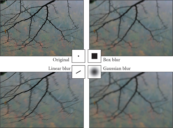
Blurring an image by convolution with each of three different filters. original. With a rescaling to avoid changing the overall brightness, we have
The opposite of blurring is sharpening, and one way to do this is by using the “unsharp mask” procedure: subtract a fraction α of a blurred image from the original. With a rescaling to avoid changing the overall brightness, we have
where fg,σ is the Gaussian filter of width σ. Using the discrete impluse d and the distributive property of convolution, we were able to write this whole process as a single filter that depends on both the width of the blur and the degree of sharpening (Figure 9.32).

Another example of combining two discrete filters is a drop shadow. It’s common to take a blurred, shifted copy of an object’s outline to create a soft drop shadow (Figure 9.33). We can express the shifting operation as convolution with an off-center impulse:

Shifting, then blurring, is achieved by convolving with both filters:
Here we have used associativity to group the two operations into a single filter with three parameters.
9.4.2 Antialiasing in Image Sampling
In image synthesis, we often have the task of producing a sampled representation of an image for which we have a continuous mathematical formula (or at least a procedure we can use to compute the color at any point, not just at integer pixel positions). Ray tracing is a common example; more about ray tracing and the specific methods for antialiasing is in Chapter 4. In the language of signal processing, we have a continuous 2D signal (the image) that we need to sample on a regular 2D lattice. If we go ahead and sample the image without any special measures, the result will exhibit various aliasing artifacts (Figure 9.34). At sharp edges in the image, we see stair-step artifacts known as “jaggies.” In areas where there are repeating patterns, we see wide bands known as moireé patterns.

Two artifacts of aliasing in images: moir patterns in periodic textures (left), and “jaggies” on straight lines (right).
The problem here is that the image contains too many small-scale features; we need to smooth it out by filtering it before sampling. Looking back at the definition of continuous convolution in Equation (9.3), we need to average the image over an area around the pixel location, rather than just taking the value at a single point. The specific methods for doing this are discussed in Chapter 4. A simple filter like a box will improve the appearance of sharp edges, but it still produces some moireé patterns (Figure 9.35). The Gaussian filter, which is very smooth, is much more effective against the moireé patterns, at the expense of overall somewhat more blurring. These two examples illustrate the tradeoff between sharpness and aliasing that is fundamental to choosing antialiasing filters.

A comparison of three different sampling filters being used to antialias a difficult test image that contains circles that are spaced closer and closer as they get larger.
9.4.3 Reconstruction and Resampling
One of the most common image operations where careful filtering is crucial is resampling—changing the sample rate, or changing the image size.
Suppose we have taken an image with a digital camera that is 3000 by 2000 pixels in size, and we want to display it on a monitor that has only 1280 by 1024 pixels. In order to make it fit, while maintaining the 3:2 aspect ratio, we need to resample it to 1278 by 852 pixels. How should we go about this?
One way to approach this problem is to think of the process as dropping pixels: the size ratio is between 2 and 3, so we’ll have to drop out one or two pixels between pixels that we keep. It’s possible to shrink an image in this way, but the quality of the result is low—the images in Figure 9.34 were made using pixel dropping. Pixel dropping is very fast, however, and it is a reasonable choice to make a preview of the resized image during an interactive manipulation.
The way to think about resizing images is as a resampling operation: we want a set of samples of the image on a particular grid that is defined by the new image dimensions, and we get them by sampling a continuous function that is reconstructed from the input samples (Figure 9.36). Looking at it this way, it’s just a sequence of standard image processing operations: first we reconstruct a continuous function from the input samples, and then we sample that function just as we would sample any other continuous image. To avoid aliasing artifacts, appropriate filters need to be used at each stage.

Resampling an image consists of two logical steps that are combined into a single operation in code. First, we use a reconstruction filter to define a smooth, continuous function from the input samples. Then, we sample that function on a new grid to get the output samples.
A small example is shown in Figure 9.37: if the original image is 12 × 9 pixels and the new one is 8 × 6 pixels, there are 2/3 as many output pixels as input pixels in each dimension, so their spacing across the image is 3/2 the spacing of the original samples.

The sample locations for the input and output grids in resampling a 12 by 9 image to make an 8 by 6 one.
In order to come up with a value for each of the output samples, we need to somehow compute values for the image in between the samples. The pixel-dropping algorithm gives us one way to do this: just take the value of the closest sample in the input image and make that the output value. This is exactly equivalent to reconstructing the image with a 1-pixel-wide (radius one-half) box filter and then point sampling.
Of course, if the main reason for choosing pixel dropping or other very simple filtering is performance, one would never implement that method as a special case of the general reconstruction-and-resampling procedure. In fact, because of the discontinuities, it’s difficult to make box filters work in a general framework. But, for high-quality resampling, the reconstruction/sampling framework provides valuable flexibility.
To work out the algorithmic details, it’s simplest to drop down to 1D and discuss resampling a sequence. The simplest way to write an implementation is in terms of the reconstruct function we defined in Section 9.2.5.
function resample(sequence a, float x0, float Δx, int n, filter f)
create sequence b of length n
for i = 0 to n – 1 do
b[i] = reconstruct(a, f, x0) + iΔx)
return b
The parameter x0 gives the position of the first sample of the new sequence in terms of the samples of the old sequence. That is, if the first output sample falls midway between samples 3 and 4 in the input sequence, x0 is 3.5.
This procedure reconstructs a continuous image by convolving the input sequence with a continuous filter and then point samples it. That’s not to say that these two operations happen sequentially—the continuous function exists only in principle and its values are computed only at the sample points. But mathematically, this function computes a set of point samples of the function a ★ f.
This point sampling seems wrong, though, because we just finished saying that a signal should be sampled with an appropriate smoothing filter to avoid aliasing. We should be convolving the reconstructed function with a sampling filter g and point sampling g ★ (f ★ a). But since this is the same as (g ★ f) ★ a, we can roll the sampling filter together with the reconstruction filter; one convolution operation is all we need (Figure 9.38). This combined reconstruction and sampling filter is known as a resampling filter.

Resampling involves filtering for reconstruction and for sampling. Since two convolution filters applied in sequence can be replaced with a single filter, we only need one resampling filter, which serves the roles of reconstruction and sampling.
When resampling images, we usually specify a source rectangle in the units of the old image that specifies the part we want to keep in the new image. For example, using the pixel sample positioning convention from Chapter 3, the rectangle we’d use to resample the entire image is . Given a source rectangle (xl, xh) × (yl, yh), the sample spacing for the new image is in x and in y. The lower-left sample is positioned at (xl + Δx/2, yl + Δy/2).
Modifying the 1D pseudocode to use this convention, and expanding the call to the reconstruct function into the double loop that is implied, we arrive at:
function resample(sequence a, float xl, float xh, int n, filter f)
create sequence b of length n
r = f.radius
x0 = xl + Δx/2
for i = 0 to n – 1 do
s = 0
x = x0 + iΔx
for j = ⌈x − r⌉ to ⌊[x + r⌋ do
s = s + a[j]f(x – j)
b[i] = s
return b
This routine contains all the basics of resampling an image. One last issue that remains to be addressed is what to do at the edges of the image, where the simple version here will access beyond the bounds of the input sequence. There are several things we might do:
- Just stop the loop at the ends of the sequence. This is equivalent to padding the image with zeros on all sides.
- Clip all array accesses to the end of the sequence—that is, return a[0] when we would want to access a[–1]. This is equivalent to padding the edges of the image by extending the last row or column.
- Modify the filter as we approach the edge so that it does not extend beyond the bounds of the sequence.
The first option leads to dim edges when we resample the whole image, which is not really satisfactory. The second option is easy to implement; the third is probably the best performing. The simplest way to modify the filter near the edge of the image is to renormalize it: divide the filter by the sum of the part of the filter that falls within the image. This way, the filter always adds up to 1 over the actual image samples, so it preserves image intensity. For performance, it is desirable to handle the band of pixels within a filter radius of the edge (which require this renormalization) separately from the center (which contains many more pixels and does not require renormalization).
The choice of filter for resampling is important. There are two separate issues: the shape of the filter and the size (radius). Because the filter serves both as a reconstruction filter and a sampling filter, the requirements of both roles affect the choice of filter. For reconstruction, we would like a filter smooth enough to avoid aliasing artifacts when we enlarge the image, and the filter should be ripple-free. For sampling, the filter should be large enough to avoid undersampling and smooth enough to avoid moireé artifacts. Figure 9.39 illustrates these two different needs.

The effects of using different sizes of a filter for upsampling (enlarging) or downsampling (reducing) an image.
Generally, we will choose one filter shape and scale it according to the relative resolutions of the input and output. The lower of the two resolutions determines the size of the filter: when the output is more coarsely sampled than the input (downsampling, or shrinking the image), the smoothing required for proper sampling is greater than the smoothing required for reconstruction, so we size the filter according to the output sample spacing (radius 3 in Figure 9.39). On the other hand, when the output is more finely sampled (upsampling, or enlarging the image) then the smoothing required for reconstruction dominates (the reconstructed function is already smooth enough to sample at a higher rate than it started), so the size of the filter is determined by the input sample spacing (radius 1 in Figure 9.39).
Choosing the filter itself is a tradeoff between speed and quality. Common choices are the box filter (when speed is paramount), the tent filter (moderate quality), or a piecewise cubic (excellent quality). In the piecewise cubic case, the degree of smoothing can be adjusted by interpolating between fB and fC; the Mitchell-Netravali filter is a good choice.
Just as with image filtering, separable filters can provide a significant speedup. The basic idea is to resample all the rows first, producing an image with changed width but not height, then to resample the columns of that image to produce the final result (Figure 9.40). Modifying the pseudocode given earlier so that it takes advantage of this optimization is reasonably straightforward.

9.5 Sampling Theory
If you are only interested in implementation, you can stop reading here; the algorithms and recommendations in the previous sections will let you implement programs that perform sampling and reconstruction and achieve excellent results. However, there is a deeper mathematical theory of sampling with a history reaching back to the first uses of sampled representations in telecommunications. Sampling theory answers many questions that are difficult to answer with reasoning based strictly on scale arguments.
But most important, sampling theory gives valuable insight into the workings of sampling and reconstruction. It gives the student who learns it an extra set of intellectual tools for reasoning about how to achieve the best results with the most efficient code.
9.5.1 The Fourier Transform
The Fourier transform, along with convolution, is the main mathematical concept that underlies sampling theory. You can read about the Fourier transform in many math books on analysis, as well as in books on signal processing.
The basic idea behind the Fourier transform is to express any function by adding together sine waves (sinusoids) of all frequencies. By using the appropriate weights for the different frequencies, we can arrange for the sinusoids to add up to any (reasonable) function we want.
As an example, the square wave in Figure 9.41 can be expressed by a sequence of sine waves:

This Fourier series starts with a sine wave (sin 2πx) that has frequency 1.0—same as the square wave—and the remaining terms add smaller and smaller corrections to reduce the ripples and, in the limit, reproduce the square wave exactly. Note that all the terms in the sum have frequencies that are integer multiples of the frequency of the square wave. This is because other frequencies would produce results that don’t have the same period as the square wave.
A surprising fact is that a signal does not have to be periodic in order to be expressed as a sum of sinusoids in this way: a non-periodic signal just requires more sinusoids. Rather than summing over a discrete sequence of sinusoids, we will instead integrate over a continuous family of sinusoids. For instance, a box function can be written as the integral of a family of cosine waves:
This integral in Equation (9.6) is adding up infinitely many cosines, weighting the cosine of frequency u by the weight (sin πu)/πu. The result, as we include higher and higher frequencies, converges to the box function (see Figure 9.42). When a function f is expressed in this way, this weight, which is a function of the frequency u, is called the Fourier transform of f, denoted . The function tells us how to build f by integrating over a family of sinusoids:

Approximating a box function with integrals of cosines up to each of four cutoff frequencies.
Equation (9.7) is known as the inverse Fourier transform (IFT) because it starts with the Fourier transform of f and ends up with f.2
Note that in Equation (9.7) the complex exponential e2πiux has been substituted for the cosine in the previous equation. Also, is a complex-valued function. The machinery of complex numbers is required to allow the phase, as well as the frequency, of the sinusoids to be controlled; this is necessary to represent any functions that are not symmetric across zero. The magnitude of is known as the Fourier spectrum, and, for our purposes, this is sufficient—we won’t need to worry about phase or use any complex numbers directly.
It turns out that computing from f looks very much like computing f from :
Equation (9.8) is known as the (forward) Fourier transform (FT). The sign in the exponential is the only difference between the forward and inverse Fourier transforms, and it is really just a technical detail. For our purposes, we can think of the FT and IFT as the same operation.
Sometimes the notation is inconvenient, and then we will denote the Fourier transform of f by ℱ{f} and the inverse Fourier transform of by .
A function and its Fourier transform are related in many useful ways. A few facts (most of them easy to verify) that we will use later in the chapter are:
A function and its Fourier transform have the same squared integral:
The physical interpretation is that the two have the same energy (Figure 9.43).
In particular, scaling a function up by a also scales its Fourier transform by a. That is, ℱ{af} = aℱ{f}.
Stretching a function along the x-axis squashes its Fourier transform along the u-axis by the same factor (Figure 9.44):

Scaling a signal along the x-axis in the space domain causes an inverse scale along the u-axis in the frequency domain.
(The renormalization by b is needed to keep the energy the same.)
This means that if we are interested in a family of functions of different width and height (say all box functions centered at zero), then we only need to know the Fourier transform of one canonical function (say the box function with width and height equal to one), and we can easily know the Fourier transforms of all the scaled and dilated versions of that function. For example, we can instantly generalize Equation (9.6) to give the Fourier transform of a box of width b and height a:
- The average value of f is equal to (0). This makes sense since (0) is supposed to be the zero-frequency component of the signal (the DC component if we are thinking of an electrical voltage).
- If f is real (which it always is for us), is an even function—that is, (u) = (−u). Likewise, if f is an even function then will be real (this is not usually the case in our domain, but remember that we really are only going to care about the magnitude of ).

9.5.2 Convolution and the Fourier Transform
One final property of the Fourier transform that deserves special mention is its relationship to convolution (Figure 9.45). Briefly,

A commutative diagram to show visually the relationship between convolution and multiplication. If we multiply f and g in space, then transform to frequency, we end up in the same place as if we transformed f and g to frequency and then convolved them. Likewise, if we convolve f and g in space and then transform into frequency, we end up in the same place as if we transformed f and g to frequency, then multiplied them.
The Fourier transform of the convolution of two functions is the product of the Fourier transforms. Following the by now familiar symmetry,
The convolution of two Fourier transforms is the Fourier transform of the product of the two functions. These facts are fairly straightforward to derive from the definitions.
This relationship is the main reason Fourier transforms are useful in studying the effects of sampling and reconstruction. We’ve seen how sampling, filtering, and reconstruction can be seen in terms of convolution; now the Fourier transform gives us a new domain—the frequency domain—in which these operations are simply products.
9.5.3 A Gallery of Fourier Transforms
Now that we have some facts about Fourier transforms, let’s look at some examples of individual functions. In particular, we’ll look at some filters from Section 9.3.1, which are shown with their Fourier transforms in Figure 9.46. We have already seen the box function:

The function3 sin x/x is important enough to have its own name, sinc x.
The tent function is the convolution of the box with itself, so its Fourier transform is just the square of the Fourier transform of the box function:
We can continue this process to get the Fourier transform of the B-spline filter (see Exercise 3):
The Gaussian has a particularly nice Fourier transform:
It is another Gaussian! The Gaussian with standard deviation 1.0 becomes a Gaussian with standard deviation 1/2π.
9.5.4 Dirac Impulses in Sampling Theory
The reason impulses are useful in sampling theory is that we can use them to talk about samples in the context of continuous functions and Fourier transforms. We represent a sample, which has a position and a value, by an impulse translated to that position and scaled by that value. A sample at position a with value b is represented by bδ(x – a). This way we can express the operation of sampling the function f(x) at a as multiplying f by δ(x – a). The result is f(a)δ(x – a).
Sampling a function at a series of equally spaced points is therefore expressed as multiplying the function by the sum of a series of equally spaced impulses, called an impulse train (Figure 9.47). An impulse train with period T, meaning that the impulses are spaced a distance T apart is

Impulse trains. The Fourier transform of an impulse train is another impulse train. Changing the period of the impulse train in space causes an inverse change in the period in frequency.
The Fourier transform of s1 is the same as s1: a sequence of impulses at all integer frequencies. You can see why this should be true by thinking about what happens when we multiply the impulse train by a sinusoid and integrate. We wind up adding up the values of the sinusoid at all the integers. This sum will exactly cancel to zero for non-integer frequencies, and it will diverge to +∞ for integer frequencies.
Because of the dilation property of the Fourier transform, we can guess that the Fourier transform of an impulse train with period T (which is like a dilation of s1) is an impulse train with period 1/T. Making the sampling finer in the space domain makes the impulses farther apart in the frequency domain.
9.5.5 Sampling and Aliasing
Now that we have built the mathematical machinery, we need to understand the sampling and reconstruction process from the viewpoint of the frequency domain. The key advantage of introducing Fourier transforms is that it makes the effects of convolution filtering on the signal much clearer, and it provides more precise explanations of why we need to filter when sampling and reconstructing.
We start the process with the original, continuous signal. In general its Fourier transform could include components at any frequency, although for most kinds of signals (especially images), we expect the content to decrease as the frequency gets higher. Images also tend to have a large component at zero frequency—remember that the zero-frequency, or DC, component is the integral of the whole image, and since images are all positive values this tends to be a large number.
Let’s see what happens to the Fourier transform if we sample and reconstruct without doing any special filtering (Figure 9.48). When we sample the signal, we model the operation as multiplication with an impulse train; the sampled signal is fsT. Because of the multiplication-convolution property, the FT of the sampled signal is .

Sampling and reconstruction with no filtering. Sampling produces alias spectra that overlap and mix with the base spectrum. Reconstruction with a box filter collects even more information from the alias spectra. The result is a signal that has serious aliasing artifacts.
Recall that δ is the identity for convolution. This means that
that is, convolving with the impulse train makes a whole series of equally spaced copies of the spectrum of f. A good intuitive interpretation of this seemingly odd result is that all those copies just express the fact (as we saw back in Section 9.1.1) that frequencies that differ by an integer multiple of the sampling frequency are indistinguishable once we have sampled—they will produce exactly the same set of samples. The original spectrum is called the base spectrum and the copies are known as alias spectra.
The trouble begins if these copies of the signal’s spectrum overlap, which will happen if the signal contains any significant content beyond half the sample frequency. When this happens, the spectra add, and the information about different frequencies is irreversibly mixed up. This is the first place aliasing can occur, and if it happens here, it’s due to undersampling—using too low a sample frequency for the signal.
Suppose we reconstruct the signal using the nearest-neighbor technique. This is equivalent to convolving with a box of width 1. (The discrete-continuous convolution used to do this is the same as a continuous convolution with the series of impulses that represent the samples.) The convolution-multiplication property means that the spectrum of the reconstructed signal will be the product of the spectrum of the sampled signal and the spectrum of the box. The resulting reconstructed Fourier transform contains the base spectrum (though somewhat attenuated at higher frequencies), plus attenuated copies of all the alias spectra. Because the box has a fairly broad Fourier transform, these attenuated bits of alias spectra are significant, and they are the second form of aliasing, due to an inadequate reconstruction filter. These alias components manifest themselves in the image as the pattern of squares that is characteristic of nearest-neighbor reconstruction.
Preventing Aliasing in Sampling
To do high quality sampling and reconstruction, we have seen that we need to choose sampling and reconstruction filters appropriately. From the standpoint of the frequency domain, the purpose of lowpass filtering when sampling is to limit the frequency range of the signal so that the alias spectra do not overlap the base spectrum. Figure 9.49 shows the effect of sample rate on the Fourier transform of the sampled signal. Higher sample rates move the alias spectra farther apart, and eventually whatever overlap is left does not matter.

The effect of sample rate on the frequency spectrum of the sampled signal. Higher sample rates push the copies of the spectrum apart, reducing problems caused by overlap.
The key criterion is that the width of the spectrum must be less than the distance between the copies—that is, the highest frequency present in the signal must be less than half the sample frequency. This is known as the Nyquist criterion, and the highest allowable frequency is known as the Nyquist frequency or Nyquist limit. The Nyquist-Shannon sampling theorem states that a signal whose frequencies do not exceed the Nyquist limit (or, said another way, a signal that is bandlimited to the Nyquist frequency) can, in principle, be reconstructed exactly from samples.
With a high enough sample rate for a particular signal, we don’t need to use a sampling filter. But if we are stuck with a signal that contains a wide range of frequencies (such as an image with sharp edges in it), we must use a sampling filter to bandlimit the signal before we can sample it. Figure 9.50 shows the effects of three lowpass (Smoothing) filters in the frequency domain, and Figure 9.51 shows the effect of using these same filters when sampling. Even if the spectra overlap without filtering, convolving the signal with a lowpass filter can narrow the spectrum enough to eliminate overlap and produce a well-sampled representation of the filtered signal. Of course, we have lost the high frequencies, but that’s better than having them get scrambled with the signal and turn into artifacts.


How the lowpass filters from Figure 9.50 prevent aliasing during sampling. Lowpass filtering narrows the spectrum so that the copies overlap less, and the high frequencies from the alias spectra interfere less with the base spectrum.
Preventing Aliasing in Reconstruction
From the frequency domain perspective, the job of a reconstruction filter is to remove the alias spectra while preserving the base spectrum. In Figure 9.48, we can see that the crudest reconstruction filter, the box, does attenuate the alias spectra. Most important, it completely blocks the DC spike for all the alias spectra. This is a characteristic of all reasonable reconstruction filters: they have zeroes in frequency space at all multiples of the sample frequency. This turns out to be equivalent to the ripple-free property in the space domain.
So a good reconstruction filter needs to be a good lowpass filter, with the added requirement of completely blocking all multiples of the sample frequency. The purpose of using a reconstruction filter different from the box filter is to more completely eliminate the alias spectra, reducing the leakage of high-frequency artifacts into the reconstructed signal, while disturbing the base spectrum as little as possible. Figure 9.52 illustrates the effects of different filters when used during reconstruction. As we have seen, the box filter is quite “leaky” and results in plenty of artifacts even if the sample rate is high enough. The tent filter, resulting in linear interpolation, attenuates high frequencies more, resulting in milder artifacts, and the B-spline filter is very smooth, controlling the alias spectra very effectively. It also smooths the base spectrum some—this is the tradeoff between smoothing and aliasing that we saw earlier.

The effects of different reconstruction filters in the frequency domain. A good reconstruction filter attenuates the alias spectra effectively while preserving the base spectrum.
Preventing Aliasing in Resampling
When the operations of reconstruction and sampling are combined in resampling, the same principles apply, but with one filter doing the work of both reconstruction and sampling. Figure 9.53 illustrates how a resampling filter must remove the alias spectra and leave the spectrum narrow enough to be sampled at the new sample rate.

Resampling viewed in the frequency domain. The resampling filter both reconstructs the signal (removes the alias spectra) and bandlimits it (reduces its width) for sampling at the new rate.
9.5.6 Ideal Filters vs. Useful Filters
Following the frequency domain analysis to its logical conclusion, a filter that is exactly a box in the frequency domain is ideal for both sampling and reconstruction. Such a filter would prevent aliasing at both stages without diminishing the frequencies below the Nyquist frequency at all.
Recall that the inverse and forward Fourier transforms are essentially identical, so the spatial domain filter that has a box as its Fourier transform is the function sin πx/πx = sinc πx.
However, the sinc filter is not generally used in practice, either for sampling or for reconstruction, because it is impractical and because, even though it is optimal according to the frequency domain criteria, it doesn’t produce the best results for many applications.
For sampling, the infinite extent of the sinc filter, and its relatively slow rate of decrease with distance from the center, is a liability. Also, for some kinds of sampling, the negative lobes are problematic. A Gaussian filter makes an excellent sampling filter even for difficult cases where high-frequency patterns must be removed from the input signal, because its Fourier transform falls off exponentially, with no bumps that tend to let aliases leak through. For less difficult cases, a tent filter generally suffices.
For reconstruction, the size of the sinc function again creates problems, but even more importantly, the many ripples create “ringing” artifacts in reconstructed signals.
Exercises
- Show that discrete convolution is commutative and associative. Do the same for continuous convolution.
- Discrete-continuous convolution can’t be commutative, because its arguments have two different types. Show that it is associative, though.
- Prove that the B-spline is the convolution of four box functions.
Show that the “flipped” definition of convolution is necessary by trying to show that convolution is commutative and associative using this (incorrect) definition (see the footnote on page 192):
- Prove that and .
- Equation 9.4 can be interpreted as the convolution of a with a filter . Write a mathematical expression for the “de-rippled” filter . Plot the filter that results from de-rippling the box, tent, and B-spline filters scaled to s = 1.25.
1 You may have noticed that one of the functions in the convolution sum seems to be flipped over—that is, b[k] gives the weight for the sample k units earlier in the sequence, while b[−k] gives the weight for the sample k units later in the sequence. The reason for this has to do with ensuring associativity; see Exercise 4. Most of the filters we use are symmetric, so you hardly ever need to worry about this.
2 Note that the term “Fourier transform” is used both for the function and for the operation that computes from f. Unfortunately, this rather ambiguous usage is standard.
3 You may notice that sin πu/πu is undefined for u = 0. It is, however, continuous across zero, and we take it as understood that we use the limiting value of this ratio, 1, at u = 0.