During the lifecycle of you data-tier applications, you may need to perform a number of maintenance tasks and performance optimizations against the tables that hold your application’s data. These operations may include partitioning a table, compressing a table, or migrating data to a memory-optimized table. In this chapter, we will explore these three concepts in detail.

Table Partitioning

Partitioning is a performance optimization for large tables and indexes that splits the object horizontally into smaller units. When the tables or indexes are subsequently accessed, SQL Server can perform an optimization called partition elimination, which allows only the required partitions to be read, as opposed to the entire table. Additionally, each partition can be stored on a separate filegroup; this allows you to store different partitions on different storage tiers. For example, you can store older, less frequently accessed data on less expensive storage. Figure 6-1 illustrates how a large Orders table may be structured.

Partitioning Concepts

Before drilling into the technical implementation of partitioning, it helps if you understand the concepts, such as partitioning keys, partition functions, partition schemes, and partition alignment. These concepts are discussed in the following sections.

Partitioning Key

The partitioning key is used to determine in which partition each row of the table should be placed. If your table has a clustered index, then the partitioning key must be a subset of the clustered index key. All other UNIQUE indexes on the table, including the primary key (if this differs from the clustered index), also need to include the partitioning key. The partitioning key can consist of any data type, with the exception of TEXT, NTEXT, IMAGE, XML, TIMESTAMP, VARCHAR(MAX), NVARCHAR(MAX), and VARBINARY(MAX). It also cannot be a user-defined CLR Type column or a column with an alias data type. It can, however, be a computed column, as long as this column is persisted. Many scenarios will use a date or datetime column as the partitioning key. This allows you to implement sliding windows based on time. We discuss sliding windows later in this chapter. In Figure 6-1, the OrderData column is being used as the partitioning key.

Because the column is used to distribute rows between partitions, you should use a column that will enable an even distribution of rows in order to gain the most benefit from the solution. The column you select should also be a column that queries will use as a filter criteria. This will allow you to achieve partition elimination.

Partition Function

You use boundary points to set the upper and lower limits of each partition. In Figure 6-1, you can see that the boundary points are set as 1st Jan 2014 and 1st Jan 2012. These boundary points are configured in a database object called the partition function. When creating the partition function, you can specify if the range should be left or right. If you align the range to the left, then any values that are exactly equal to a boundary point value will be stored in the partition to the left of that boundary point. If you align the range with the right, then values exactly equal to the boundary point value will be placed in the partition to the right of that boundary point. The partition function also dictates the data type of the partitioning key.

Partition Scheme

Each partition can be stored on a separate filegroup. The partition scheme is an object that you create to specify which filegroup each partition will be stored on. As you can see from Figure 6-1, there is always one more partition than there is boundary point. When you create a partition scheme, however, it is possible to specify an “extra” filegroup. This will define the next filegroup that should be used if an additional boundary point is added. It is also possible to specify the ALL keyword, as opposed to specifying individual filegroups. This will force all partitions to be stored on the same filegroup.

Index Alignment

An index is considered aligned with the table if it is built on the same partition function as the table. It is also considered aligned if it is built on a different partition function, but the two functions are identical, in that they share the same data type, the same number of partitions, and the same boundary point values.

Because the leaf level of a clustered index consists of the actual data pages of the table, a clustered index is always aligned with the table. A nonclustered index, however, can be stored on a separate filegroup to the heap, or clustered index. This extends to partitioning, where either the base table or nonclustered indexes can be independently partitioned. If nonclustered indexes are stored on the same partition scheme or an identical partition scheme, then they are aligned. If this is not the case, then they are nonaligned.

Aligning indexes with the base table is good practice unless you have a specific reason not to. This is because aligning indexes can assist with partition elimination. Index alignment is also required for operations such as SWITCH, which will be discussed later in this chapter.

Partitioning Hierarchy

Objects involved in partitioning work in a one-to-many hierarchy, so multiple tables can share a partition scheme and multiple partition schemes can share a partition function, as illustrated in Figure 6-2.

Implementing Partitioning

Implementing partitioning involves creating the partition function and partition scheme and then creating the table on the partition scheme. If the table already exists, then you will need to drop and re-create the table’s clustered index. These tasks are discussed in the following sections.

Creating the Partitioning Objects

The first object that you will need to create is the partition function. This can be created using the CREATE PARTITION FUNCTION statement, as demonstrated in Listing 6-1. This script creates a database called Chapter6 and then creates a partition function called PartFunc. The function specifies a data type for partitioning keys of DATE and sets boundary points for 1st Jan 2014 and 1st Jan 2012. Table 6-1 details how dates will be distributed between partitions.

USE Master
GO

--Create Database Chapter 6 using default settings from Model

CREATE DATABASE Chapter6 ;
GO

USE Chapter6
GO

--Create Partition Function

CREATE PARTITION FUNCTION PartFunc(Date)
AS RANGE LEFT
FOR VALUES(’2012-01-01’, ’2014-01-01’) ;

The next object that we need to create is a partition scheme. This can be created using the CREATE PARTITION SCHEME statement, as demonstrated in Listing 6-2. This script creates a partition scheme called PartScheme against the PartFunc partition function and specifies that all partitions will be stored on the PRIMARY filegroup. Although storing all partitions on the same filegroup does not allow us to implement storage tiering, it does enable us to automate sliding windows.

CREATE PARTITION SCHEME PartScheme
AS PARTITION PartFunc
ALL TO ([PRIMARY]) ;

Creating a New Partitioned Table

Now that we have a partition function and partition scheme in place, all that remains is to create our partitioned table. The script in Listing 6-3 creates a table called Orders and partitions it based on the OrderDate column. Even though OrderNumber provides a natural primary key for our table, we need to include OrderDate in the key so that it can be used as our partitioning column. Obviously, the OrderDate column is not be suitable for the primary key on its own, since it is not guaranteed to be unique.

CREATE TABLE dbo.Orders
        (
        OrderNumber int         NOT NULL,
        OrderDate date          NOT NULL,
        CustomerID int          NOT NULL,
        ProductID int           NOT NULL,
        Quantity int            NOT NULL,
        NetAmount money         NOT NULL,
        TaxAmount money         NOT NULL,
        InvoiceAddressID int    NOT NULL,
        DeliveryAddressID int   NOT NULL,
        DeliveryDate date       NULL
        )  ON PartScheme(OrderDate)  ;
GO

ALTER TABLE dbo.Orders ADD CONSTRAINT
        PK_Orders PRIMARY KEY CLUSTERED
         (
        OrderNumber,
        OrderDate
        ) WITH( STATISTICS_NORECOMPUTE = OFF, IGNORE_DUP_KEY = OFF,
                    ALLOW_ROW_LOCKS = ON, ALLOW_PAGE_LOCKS = ON) ON PartScheme(OrderDate) ;

GO

The important thing to notice in this script is the ON clause. Normally, you would create a table “on” a filegroup, but in this case, we are creating the table “on” the partition scheme and passing in the name of the column that will be used as the partitioning key. The data type of the partitioning key must match the data type specified in the partition function.

Partitioning an Existing Table

Because the clustered index is always aligned with the base table, the process of moving a table to a partition scheme is as simple as dropping the clustered index and then re-creating the clustered index on the partition scheme. The script in Listing 6-4 creates a table called ExistingOrders and populates it with data.

--Create the ExistingOrders table

CREATE TABLE dbo.ExistingOrders
        (
        OrderNumber int         IDENTITY        NOT NULL,
        OrderDate date           NOT NULL,
        CustomerID int            NOT NULL,
        ProductID int               NOT NULL,
        Quantity int                  NOT NULL,
        NetAmount money      NOT NULL,
        TaxAmount money      NOT NULL,
        InvoiceAddressID int   NOT NULL,
        DeliveryAddressID int  NOT NULL,
        DeliveryDate date        NULL
        )  ON [PRIMARY] ;
GO

ALTER TABLE dbo.ExistingOrders ADD CONSTRAINT
        PK_ExistingOrders PRIMARY KEY CLUSTERED
         (
        OrderNumber,
        OrderDate
        ) WITH( STATISTICS_NORECOMPUTE = OFF, IGNORE_DUP_KEY = OFF,
                    ALLOW_ROW_LOCKS = ON, ALLOW_PAGE_LOCKS = ON) ON [PRIMARY] ;

GO

--We will now populate the data with data so that we can view the storage properties
--and then partition the table when the data already exists.

--Build a numbers table for the data population

DECLARE @Numbers TABLE
(
        Number        INT
)

;WITH CTE(Number)
AS
(
        SELECT 1 Number
        UNION ALL
        SELECT Number + 1
        FROM CTE
        WHERE Number < 20
)
INSERT INTO @Numbers
SELECT Number FROM CTE ;

--Populate ExistingOrders with data

INSERT INTO dbo.ExistingOrders
SELECT
         (SELECT CAST(DATEADD(dd,(SELECT TOP 1 Number
                                  FROM @Numbers
                                  ORDER BY NEWID()),getdate())as DATE)),
         (SELECT TOP 1 Number -10 FROM @Numbers ORDER BY NEWID()),
         (SELECT TOP 1 Number FROM @Numbers ORDER BY NEWID()),
         (SELECT TOP 1 Number FROM @Numbers ORDER BY NEWID()),
        500,
        100,
         (SELECT TOP 1 Number FROM @Numbers ORDER BY NEWID()),
         (SELECT TOP 1 Number FROM @Numbers ORDER BY NEWID()),
         (SELECT CAST(DATEADD(dd,(SELECT TOP 1 Number - 10
                                  FROM @Numbers
                                  ORDER BY NEWID()),getdate()) as DATE))
FROM @Numbers a
CROSS JOIN @Numbers b ;

As shown in Figure 6-3, by looking at the Storage tab of the Table Properties dialog box, we can see that the table has been created on the PRIMARY filegroup and is not partitioned.

The script in Listing 6-5 now drops the clustered index of the ExistingOrders table and re-creates it on the PartScheme partition scheme. Again, the key line to note is the ON clause, which specifies PartScheme as the target partition function and passes in OrderDate as the partitioning key.

--Drop Clustered Index

ALTER TABLE dbo.ExistingOrders DROP CONSTRAINT PK_ExistingOrders ;
GO

--Re-created clustered index on PartScheme

ALTER TABLE dbo.ExistingOrders ADD  CONSTRAINT PK_ExistingOrders PRIMARY KEY CLUSTERED
(
        OrderNumber ASC,
        OrderDate ASC
)WITH (PAD_INDEX = OFF, STATISTICS_NORECOMPUTE = OFF, SORT_IN_TEMPDB = OFF,
            IGNORE_DUP_KEY = OFF, ONLINE = OFF, ALLOW_ROW_LOCKS = ON,
            ALLOW_PAGE_LOCKS = ON) ON PartScheme(OrderDate) ;
GO

In Figure 6-4, you can see that if you look again at the Storage tab of the Table Properties dialog box, you find that the table is now partitioned against the PartScheme partition scheme.

Monitoring Partitioned Tables

You may wish to keep track of the number of rows in each partition of your table. Doing so allows you to ensure that your rows are being distributed evenly. If they are not, then you may wish to reassess you partitioning strategy to ensure you get the full benefit from the technology. There are two methods that you can use for this: the $PARTITION function and the Disk Usage by Partition SSMS Report.

$PARTITION Function

You can determine how many rows are in each partition of your table by using the $PARTITION function. When you run this function against the partition function, it accepts the column name of your partitioning key as a parameter, as demonstrated in Listing 6-6.

SELECT
        COUNT(*) ’Number of Rows’
        ,$PARTITION.PartFunc(OrderDate) ’Partition’
FROM dbo.ExistingOrders
GROUP BY $PARTITION.PartFunc(OrderDate) ;

From the results in Figure 6-5, you can see that all of the rows in our table sit in the same partition, which pretty much defies the point of partitioning and means that we should reassess our strategy.

We can also use the $PARTITION function to assess how a table would be partitioned against a different partition function. This can help us plan to resolve the issue with our ExistingOrders table. The script in Listing 6-7 creates a new partition function, called PartFuncWeek, which creates weekly partitions for the month of November 2014. It then uses the $PARTITION function to determine how the rows of our ExistingOrders table will be split if we implemented this strategy. For the time being, we do not need to create a partition scheme or repartition the table. Before running the script, change the boundary point values so they are based upon the date when you run the script. This is because the data in the table is generated using the GETDATE() function.

--Create new partition function
CREATE PARTITION FUNCTION PartFuncWeek(DATE)
AS RANGE LEFT
FOR VALUES (’2014-11-7’,’2014-11-14’,’2014-11-21’,’2014-11-28’) ;

--Assess spread of rows
SELECT
        COUNT(*) ’Number of Rows’
        ,$PARTITION.PartFuncWeek(OrderDate) ’Partition’
FROM dbo.ExistingOrders
GROUP BY $PARTITION.PartFuncWeek(OrderDate) ;

The results in Figure 6-6 show that the rows of the ExistingOrders table are fairly evenly distributed among the weekly partitions, so this may provide a suitable strategy for our table.

Sliding Windows

Our weekly partitioning strategy seems to work well, but what about when we reach December? As it currently stands, all new order placed after 28th November 2014 will all end up in the same partition, which will just grow and grow. To combat this issue, SQL Server provides us with the tools to create sliding windows. In our case, this means that each week, a new partition will be created for the following week and the earliest partition will be removed.

To achieve this, we can use the SPLIT, MERGE, and SWITCH operations. The SPLIT operation adds a new boundary point, thus creating a new partition. The MERGE operation removes a boundary point, thus merging two partitions together. The SWITCH operation moves a partition into an empty table or partition.

In our scenario, we create a staging table, called OldOrdersStaging. We use this table as a staging area to hold the data from our earliest partition. Once in the staging table, you can perform whatever operations or transformation may be required. For example, your developers may wish to create a script, to roll the data up, and to transfer it to a historical Orders table. Even though the OldOrdersStaging table is designed as a temporary object, it is important to note that you cannot use a temporary table. Instead, you must use a permanent table and drop it at the end. This is because temporary tables reside in TempDB, which means that they will be on a different filegroup, and SWITCH will not work. SWITCH is a metadata operation, and therefore, both partitions involved must reside on the same filegroup.

The script in Listing 6-8 implements a sliding window. First, it creates a staging table for the older orders. The indexes and constraints of this table must be the same as those of the partitioned table. The table must also reside on the same filegroup in order for the SWITCH operation to succeed. It then determines the highest and lowest boundary point values in the partitioned table, which it will use as parameters for the SPLIT and MERGE operations. It then uses the ALTER PARTITION FUNCTION command to remove the lowest boundary point value and add in the new boundary point. Finally, it reruns the $PARTITION function to display the new distribution of rows and interrogates the sys.partition_functions and sys.partition_range_values catalog views to display the new boundary point values for the PartFuncWeek partition function. The script assumes that the PartSchemeWeek partition scheme has been created and the ExistingOrders table has been moved to this partition scheme.

--Create the OldOrders table

CREATE TABLE dbo.OldOrdersStaging(
        [OrderNumber] [int] IDENTITY(1,1) NOT NULL,
         [OrderDate] [date] NOT NULL,
         [CustomerID] [int] NOT NULL,
         [ProductID] [int] NOT NULL,
         [Quantity] [int] NOT NULL,
         [NetAmount] [money] NOT NULL,
         [TaxAmount] [money] NOT NULL,
         [InvoiceAddressID] [int] NOT NULL,
         [DeliveryAddressID] [int] NOT NULL,
         [DeliveryDate] [date] NULL,
 CONSTRAINT PK_OldOrdersStaging PRIMARY KEY CLUSTERED
(
        OrderNumber ASC,
        OrderDate ASC
)WITH (PAD_INDEX = OFF, STATISTICS_NORECOMPUTE = OFF, IGNORE_DUP_KEY = OFF,
           ALLOW_ROW_LOCKS = ON, ALLOW_PAGE_LOCKS = ON)
) ;
GO

--Calculate the lowest boundary point value

DECLARE @LowestBoundaryPoint DATE = (
        SELECT TOP 1 CAST(value  AS DATE)
        FROM sys.partition_functions pf
        INNER JOIN sys.partition_range_values prv
                ON pf.function_id = prv.function_id
        WHERE pf.name = ’PartFuncWeek’
        ORDER BY value ASC) ;

--Calculate the newest boundary point value

DECLARE @HighestboundaryPoint DATE = (
SELECT TOP 1 CAST(value  AS DATE)
        FROM sys.partition_functions pf
        INNER JOIN sys.partition_range_values prv
                ON pf.function_id = prv.function_id
        WHERE pf.name = ’PartFuncWeek’
        ORDER BY value DESC) ;

--Add 7 days to the newest boundary point value to determine the new boundary point

DECLARE @NewSplitRange DATE = (
        SELECT DATEADD(dd,7,@HighestboundaryPoint)) ;

--Switch the oldest partition to the OldOrders table

ALTER TABLE ExistingOrders
        SWITCH PARTITION 1 TO OldOrdersStaging PARTITION 2 ;

--Remove the oldest partition

ALTER PARTITION FUNCTION PartFuncWeek()
        MERGE RANGE(@LowestBoundaryPoint) ;

--Create the new partition

ALTER PARTITION FUNCTION PartFuncWeek()
        SPLIT RANGE(@NewSplitRange) ;
GO

--Re-run $PARTITION to assess new spread of rows

SELECT
        COUNT(*) ’Number of Rows’
        ,$PARTITION.PartFuncWeek(OrderDate) ’Partition’
FROM dbo.ExistingOrders
GROUP BY $PARTITION.PartFuncWeek(OrderDate) ;

SELECT name, value FROM SYS.partition_functions PF
INNER JOIN SYS.partition_range_values PFR ON PF.function_id = PFR.function_id
WHERE name = ’PARTFUNCWEEK’ ;

The results displayed in Figure 6-7 show how the partitions have been realigned.

When you are using the SWITCH function, there are several limitations. First, all nonclustered indexes of the table must be aligned with the base table. Also, the empty table or partition that you move the data into must have the same indexing structure. It must also reside on the same filegroup as the partition that you are switching out. This is because the SWITCH function does not actually move any data. It is a metadata operation that changes the pointers of the pages that make up the partition.

You can use MERGE and SPLIT with different filegroups, but there will be a performance impediment. Like SWITCH, MERGE and SPLIT can be performed as metadata operations if all partitions involved reside on the same filegroup. If they are on different filegroups, however, then physical data moves need to be performed by SQL Server, which can take substantially longer.

Partition Elimination

One of the key benefits of partitioning is that the Query Optimizer is able to access only the partitions require to satisfy the results of a query, instead of the entire table. For partition elimination to be successful, the partitioning key must be included as a filter in the WHERE clause. We can witness this functionality by running the query in Listing 6-9 against our ExistingOrders table and choosing the option to include the actual execution plan.

SELECT OrderNumber, OrderDate
FROM dbo.ExistingOrders
WHERE OrderDate BETWEEN ’2014-11-01’ AND ’2014-11-14’ ;

If we now view the execution plan and examine the properties of the Index Scan operator through Management Studio 2014, we see that only one partition has been accessed, as shown in Figure 6-8.

The partition elimination functionality can be a little fragile, however. For example, if you are manipulating the OrderDate column in any way, as opposed to just using it for evaluation, then partition elimination cannot occur. For example, if you cast the OrderDate column to the DATETIME2 data type, as demonstrated in Listing 6-10, then all partitions would need to be accessed.

SELECT OrderNumber, OrderDate
FROM dbo.ExistingOrders
WHERE CAST(OrderDate AS DATETIME2) BETWEEN ’2014-11-01’ AND ’2014-11-14’ ;

Figure 6-9 illustrates the same properties of the Index Scan operator, viewed through Management Studio 2014. Here you can see that all partitions have been accessed, as opposed to just one.

Table Compression

When you think of compression, it is natural to think of saving space at the expense of performance. However, this does not always hold true for SQL Server table compression. Compression in SQL Server can actually offer a performance benefit. This is because SQL Server is usually an IO-bound application, as opposed to being CPU bound. This means that if SQL Server needs to read dramatically fewer pages from disk, then performance will increase, even if this is at the expense of CPU cycles. Of course, if your database is, in fact, CPU bound because you have very fast disks and only a single CPU core, for example, then compression could have a negative impact, but this is atypical. In order to understand table compression, it helps to have insight into how SQL Server stores data within a page. Although a full discussion of page internals is beyond the scope of this book, Figure 6-10 gives you a high-level view of the default structure of an on-disk page and row.

Within the row, the row metadata contains details such as whether or not versioning information exists for the row and if the row has NULL values. The fixed-length column metadata records the length of the fixed-length portion of the page. The variable-length metadata includes a column offset array for the variable-length columns so that SQL Server can track where each column begins in relation to the beginning of the row.

Row Compression

On an uncompressed page, as just described, SQL Server stores fixed-length columns first, followed by variable-length columns. The only columns that can be variable length are columns with a variable-length data type, such as VARCHAR or VARBINARY. When row compression is implemented for a table, SQL Server uses the minimum amount of storage for other data types as well. For example, if you have an integer column that contains a NULL value in row 1, a value of 50 in row 2, and a value of 40,000 in row 3, then in row 1, the column does not use any space at all; it uses 1 byte in row 2, because it will store this value as a TINYINT; and it uses 4 bytes in row 3, because it will need to store this value as an INT. This is opposed to an uncompressed table using 4 bytes for every row, including row 1.

In addition, SQL Server also compresses Unicode columns so that characters that can be stored as a single byte only use a single byte, as opposed to 2 bytes, as they would in an uncompressed page. In order to achieve these optimizations, SQL Server has to use a different page format, which is outlined in Figure 6-11.

In Figure 6-11, the first area of row metadata contains details such as whether or not there is versioning information about the row and if any long data columns exist. The column descriptor contains the number of short columns and the length of each long column. The second area of metadata contains details such as versioning information and forwarding pointers for heaps.

Page Compression

When you implement page compression, row compression is implemented first. Page compression itself is actually comprised of two different forms of compression. The first is prefix compression and the second is dictionary compression. These compression types are outlined in the following sections.

Prefix Compression

Prefix compression works by establishing a common prefix for a column across rows within a page. Once the best prefix value has been established, SQL Server chooses the longest value that contains the full prefix as the anchor row and stores all other values within the column, as a differential of the anchor row, as opposed to storing the values themselves. For example, Table 6-2 details the values that are being stored within a column and follows this with a description of how SQL Server will store the values using prefix compression. The value Postfreeze has been chosen as the anchor value, since it is the longest value that contains the full prefix of Post, which has been identified. The number in <> is a marker of how many characters of the prefix are used.

Dictionary Compression

Dictionary compression is performed after all columns have been compressed using prefix compression. It looks across all columns within a page and finds values that match. The matching is performed using the binary representation of a value, which makes the process data-type agnostic. When it finds duplicate values, it adds them to a special dictionary at the top of the page, and in the row, it simply stores a pointer to the value’s location in the dictionary. Table 6-3 expands on the previous table to give you an overview of this.

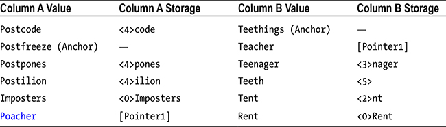
Here, you can see that the value <2>acher, which appeared in both columns in the previous table, has been replaced with a pointer to the dictionary where the value is stored.

Page Compression Structure

In order to facilitate page compression, a special row is inserted in the page immediately after the page header, which contains the information regarding the anchor record and dictionary. This row is called the compression information record, and it is illustrated in Figure 6-12.

The row metadata for the compression information record specifies if the record contains an anchor record and a dictionary. The change count records how many changes have been made to the page, which may affect the usefulness of the anchor and dictionary. When a table is rebuilt, SQL Server can use this information to determine if the page should be rebuilt. The offsets contain the start and end locations of the dictionary, from the beginning of the page. The anchor record contains each column’s prefix value and the dictionary contains the duplicate values for which pointers have been created.

Columnstore Compression

Columnstore indexes are always compressed, automatically. This means that if you create a clustered columnstore index on your table, your table is also compressed, and this cannot be combined with row or page compression. There are two types of columnstore compression available to you; COLUMNSTORE, which was introduced in SQL Server 2012, and COLUMNSTORE_ARCHIVE, which was introduced in SQL Server 2014.

You can think of COLUMNSTORE as the standard compression type for columnstore indexes and you should only use the COLUMNSTORE_ARCHIVE algorithm for data that is infrequently accessed. This is because this new compression algorithm in SQL Server 2014 breaks the rules for SQL Server data compression as far as performance goes. If you implement this algorithm, expect a very high compression ratio, but prepare for it to be at the expense of query performance.

Implementing Compression

The planning and implementation of row and page compression is a fairly straightforward process, and it is discussed in the following sections.

Selecting the Compression Level

As you probably realized from the earlier descriptions of row and page compression, page compression offers a higher compression ratio than row compression, which means better IO performance. However, this is at the expense of CPU cycles, both when the table is being compressed, and again when it is being accessed. Therefore, before you start compressing your tables, make sure you understand how much each of these compression types will reduce the size of your table by so that you can assess how much IO efficiency you can achieve.

You can accomplish this by using a system stored procedure called sp_estimate_data_compression_savings. This procedure estimates the amount of space that you could save by implementing compression. It accepts the parameters listed in Table 6-4.

The two executions of the sp_estimate_data_compression_savings stored procedure in Listing 6-11 assess the impact of row and page compression, respectively, on all partitions of our ExistingOrders table.

EXEC sp_estimate_data_compression_savings @schema_name = ’dbo’, @object_name = ’ExistingOrders’,
     @index_id = NULL, @partition_number = NULL, @data_compression =’ROW’ ;

EXEC sp_estimate_data_compression_savings @schema_name = ’dbo’, @object_name = ’ExistingOrders’,
     @index_id = NULL, @partition_number = NULL, @data_compression =’PAGE’ ;

The results in Figure 6-13 show that for the two partitions that are currently in use, page compression will have no additional benefit over row compression. Therefore, it is pointless to add the extra CPU overhead associated with page compression. This is because row compression is always implemented on every row of every page in the table. Page compression, on the other hand, is assessed on a page-by-page basis, and only pages that will benefit from being compressed are rebuilt. Because of the random nature of the largely numeric data that we inserted into this table, SQL Server has determined that the pages of our table will not benefit from page compression.

Compressing Tables and Partitions

We determined that row compression reduces the size of our table, but we can’t gain any further benefits by implementing page compression. Therefore, we can compress our entire table using the command in Listing 6-12.

ALTER TABLE ExistingOrders
    REBUILD WITH (DATA_COMPRESSION = ROW) ;

If we look more closely at the results, however, we can see that, in fact, only partition 1 benefits from row compression. Partition 2 remains the same size. Therefore, it is not worth the overhead to compress partition 2. Running the ALTER TABLE statement in Listing 6-13 will rebuild only partition 1. It will then remove compression from the entire table by rebuilding it with DATA_COMPRESSION = NONE.

--Compress partition 1 with ROW compression

ALTER TABLE ExistingOrders
    REBUILD PARTITION = 1 WITH (DATA_COMPRESSION = ROW) ;
GO

--Remove compression from the whole table

ALTER TABLE ExistingOrders
    REBUILD WITH (DATA_COMPRESSION = NONE) ;

Data Compression Wizard

The Data Compression Wizard can be reached via the context menu of a table by drilling down through Storage | Manage Compression. It provides a graphical user interface (GUI) for managing compression. The main page of the wizard is illustrated in Figure 6-14. On this screen, you can utilize the Use Same Compression Type For All Partitions option to implement one type of compression uniformly across the table. Alternatively, you can specify different compression types for each individual partition. The Calculate button runs the sp_estimate_data_compression_savings stored procedure and displays the current and estimated results for each partition.

On the final page of the wizard, you can choose to run the process immediately, script the action, or schedule it to run using SQL Server Agent.

Maintaining Compression on Heaps

When new pages are added to a heap (a table without a Clustered Index), they are not automatically compressed with page compression. This means that rebuilding a compressed table should be part of your standard maintenance routines when it does not have a clustered index. To rebuild the compression on a table, you should remove compression and then re-implement it.

Maintaining Compressed Partitions

In order to use the SWITCH operation with partitions, both partitions must have the same level of compression selected. If you use MERGE, then the compression level of the destination partition is used. When you use SPLIT, the new partition inherits its compression level from the original partition.

Just like with a non-partitioned table, if you drop the clustered index of a table, then the heap inherits the compression level of the clustered index. However, if you drop the clustered index as part of an exercise to modify the partition scheme, then compression is removed from the table.

Memory-Optimized Tables

In-Memory OLTP is a new feature of SQL Server 2014 that can offer significant performance improvements by storing all of the table’s data in memory. This, of course, can dramatically reduce IO, despite the fact that the tables are also saved to disk for durability. This is because the disk-based version of the tables is stored in an unstructured format, outside of the database engine, using a FILESTREAM-based technology. Also, memory-optimized checkpoints happen a lot more frequently. An automatic checkpoint is taken after the transaction log has grown by 512MB since the last time an automatic checkpoint occurred. This removes IO spikes that are associated with checkpoint activity. IO contention on transaction logs can also be reduced with memory optimized tables since less data is logged.

In addition to minimizing IO, In-Memory OLTP can also reduce CPU overhead. This is because natively compiled stored procedures can be used to access the data, as opposed to traditional, interpreted code. Natively compiled stored procedures use significantly fewer instructions, meaning less CPU time. Memory-optimized tables do not help reduce network overhead, however, because the same amount of data still needs to be communicated to the client.

By their very nature, memory-optimized tables increase memory pressure as opposed to reducing it, because even if you never use the data, it still sits in memory, reducing the amount of space available in which traditional resources can be cached. This means that in-memory functionality is designed for OLTP workloads as opposed to data warehousing workloads. The expectation is that fact and dimension tables within a data warehouse are too large to reside in memory.

As well as lower resource usage, memory-optimized tables can also help reduce contention. When you access data in a memory-optimized table, SQL Server does not take out a latch. This means that both latch and spinlock contention is automatically removed. Blocking between read and write transactions can also be reduced because of a new optimistic concurrency method for implementing isolation levels. Transactions and isolation levels, including memory optimized, are discussed in Chapter 18.

Durability

When creating memory optimized tables, you can specify either SCHEMA_AND_DATA or SCHEMA_ONLY as the durability setting. If you select SCHEMA_AND_DATA, then all of the table’s data is persisted to disk and transactions are logged. If you select SCHEMA_ONLY, however, then data is not persisted, and transactions are not logged. This means that after the SQL Server service is restarted, the structure of the table will remain intact, but it will contain no data. This can be useful for transient processes, such as data staging during an ETL load.

Creating and Managing Memory-Optimized Tables

Before you can create a memory-optimized table, a memory-optimized filegroup must already exist. Memory optimized filegroups are discussed in Chapter 5.

You create memory-optimized tables using the CREATE TABLE T-SQL statement, as you would for a disk-based table. The difference is that you must specify a WITH clause, which specifies that the table will be memory optimized. The WITH clause is also used to indicate the level of durability that you require.

Memory-optimized tables must also include an index. We fully discuss indexes, including indexes for memory-optimized tables, in Chapter 7, but for now, you should know that memory-optimized tables support the following types of indexes:

• Nonclustered hash index
• Nonclustered index

Hash indexes are organized into buckets, and when you create them, you must specify a bucket count using the BUCKET_COUNT parameter. Ideally, your bucket count should be two times the number of distinct values within the index key. You will not always know how many distinct values you have; in such cases, you may wish to significantly increase the BUCKET_COUNT. The tradeoff is that the more buckets you have, the more memory the index consumes. Once you have created the table, the index will be a fixed size and it is not possible to alter the table or its indexes.

The script in Listing 6-14 creates a memory-optimized table called OrdersMem with full durability and populates it with data. It creates a nonclustered hash index on the ID column with a bucket count of 2,000,000, since we will be inserting 1,000,000 rows. The script assumes that the memory-optimized filegroup has already been created.

USE [Chapter6]
GO

CREATE TABLE dbo.OrdersMem(
        OrderNumber int IDENTITY(1,1) NOT NULL PRIMARY KEY NONCLUSTERED HASH
                                                   WITH (BUCKET_COUNT= 2000000),
        OrderDate date NOT NULL,
        CustomerID int NOT NULL,
        ProductID int NOT NULL,
        Quantity int NOT NULL,
        NetAmount money NOT NULL,
        TaxAmount money NOT NULL,
        InvoiceAddressID int NOT NULL,
        DeliveryAddressID int NOT NULL,
        DeliveryDate date NULL,
)WITH (MEMORY_OPTIMIZED = ON, DURABILITY = SCHEMA_AND_DATA) ;

DECLARE @Numbers TABLE
(
        Number        INT
)

;WITH CTE(Number)
AS
(
        SELECT 1 Number
        UNION ALL
        SELECT Number + 1
        FROM CTE
        WHERE Number < 100
)
INSERT INTO @Numbers
SELECT Number FROM CTE ;

--Populate ExistingOrders with data

INSERT INTO dbo.OrdersMem
SELECT
         (SELECT CAST(DATEADD(dd,(SELECT TOP 1 Number
                                  FROM @Numbers
                                  ORDER BY NEWID()),getdate())as DATE)),
         (SELECT TOP 1 Number -10 FROM @Numbers ORDER BY NEWID()),
         (SELECT TOP 1 Number FROM @Numbers ORDER BY NEWID()),
         (SELECT TOP 1 Number FROM @Numbers ORDER BY NEWID()),
        500,
        100,
         (SELECT TOP 1 Number FROM @Numbers ORDER BY NEWID()),
         (SELECT TOP 1 Number FROM @Numbers ORDER BY NEWID()),
         (SELECT CAST(DATEADD(dd,(SELECT TOP 1 Number - 10
                                  FROM @Numbers
                                  ORDER BY NEWID()),getdate()) as DATE))
FROM @Numbers a
CROSS JOIN @Numbers b
CROSS JOIN @Numbers c ;

Performance Profile

While memory-optimized tables were in development, they were known as Hekaton, which is a play on words, meaning 100 times faster. So let’s see how performance compares for different query types between in-memory and disk-based tables. The code in Listing 6-15 creates a new table, called OrdersDisc, and populates it with the data from OrdersMem so that you can run fair tests against the two tables.

USE [Chapter6]
GO

CREATE TABLE dbo.OrdersDisc(
        OrderNumber int NOT NULL,
        OrderDate date NOT NULL,
        CustomerID int NOT NULL,
        ProductID int NOT NULL,
        Quantity int NOT NULL,
        NetAmount money NOT NULL,
        TaxAmount money NOT NULL,
        InvoiceAddressID int NOT NULL,
        DeliveryAddressID int NOT NULL,
        DeliveryDate date NULL,
 CONSTRAINT [PK_OrdersDisc] PRIMARY KEY CLUSTERED
(
         [OrderNumber] ASC,
         [OrderDate] ASC
)
) ;

INSERT INTO dbo.OrdersDisc
        SELECT *
        FROM dbo.OrdersMem ;

First, we will run the most basic test—a SELECT * query from each table. The script in Listing 6-16 runs these queries after tearing down the plan cache and the buffer cache to ensure a fair test.

SET STATISTICS TIME ON

--Tear down the plan cache

DBCC FREEPROCCACHE

--Tear down the buffer cache

DBCC DROPCLEANBUFFERS

--Run the benchmarks

SELECT *
FROM dbo.OrdersMem ;

SELECT *
FROM dbo.OrdersDisc ;

From the results in Figure 6-15, you can see that the memory-optimized table returned the results just under 4.5 percent faster.

In the next test, we see what happens if we add in an aggregation. The script in Listing 6-17 runs COUNT(*) queries against each of the tables.

SET STATISTICS TIME ON

--Tear down the plan cache

DBCC FREEPROCCACHE

--Tear down the buffer cache

DBCC DROPCLEANBUFFERS

--Run the benchmarks

SELECT COUNT(*)
FROM dbo.OrdersMem ;

SELECT COUNT(*)
FROM dbo.OrdersDisc ;

From the results in Figure 6-16, we can see that this time, the memory-optimized tabled performed considerably better than the disk-based table, offering us a 340-percent performance improvement over the disk-based table.

It is also interesting to see how memory-optimized tables compare to disk-based tables when there is a filter on the OrderNumber column, since this column is cover by an index on both tables. The script in Listing 6-18 adds the data in the NetAmount column, but it also filters on the OrderNumber column so that only OrderNumbers over 950,000 are considered.

SET STATISTICS TIME ON

--Tear down the plan cache

DBCC FREEPROCCACHE

--Tear down the buffer cache

DBCC DROPCLEANBUFFERS

--Run the benchmarks

SELECT SUM(NetAmount)
FROM dbo.OrdersMem
WHERE OrderNumber > 950000 ;

SELECT SUM(NetAmount)
FROM dbo.OrdersDisc
WHERE OrderNumber > 950000 ;

In this instance, because the memory-optimized table was scanned but the clustered index on the disk-based table was able to perform an index seek, the disk-based table performed approximately ten times faster than the memory-optimized table. This is illustrated in Figure 6-17.

Table Memory Optimization Advisor

The Table Memory Optimization Advisor is a wizard that can run against an existing disk-based table and it will walk you through the process of migration. The first page of the wizard checks your table for incompatible features, such as sparse columns and foreign key constraints, as illustrated in Figure 6-18.

The following page provides you with a warning having to do with which features are not available for memory-optimized tables, such as cross database transaction and TRUNCATE TABLE statements, as shown in Figure 6-19.

The Migration Options page of the wizard allows you to specify the durability level of the table. Checking the box causes the table to be created with DURABILITY = SCHEMA_ONLY. On this screen, you can also choose a new name for the disk-based table that you are migrating, since obviously, the new object cannot share the name of the existing object. Finally, you can use the check box to specify if you want the data from the existing table to be copied to the new table. This page of the wizard is illustrated in Figure 6-20.

The Primary Key Migration page allows you to select the columns that you wish to use to form the primary key of the table as well as the index that you want to create on your table. If you choose a nonclustered hash index, you need to specify the bucket count, whereas if you choose a nonclustered index, you need to specify the columns and order. The Primary Key Migration screen is shown in Figure 6-21.

The Summary screen of the wizard provides an overview of the activities that will be performed. Clicking the Migrate button causes the table to be migrated.

Limitations of Memory-Optimized Tables

Not all features are compatible with memory-optimized tables. The following lists the data types that cannot be used with memory-optimized tables:

• DATETIMEOFFSET
• HIERARCHYID
• SQL_VARIANT
• GEOGRAPHY
• GEOMETRY
• ROWVERSION
• (N)VARCHAR(MAX)
• VARBINARY(MAX)
• IMAGE
• (N)TEXT
• XML

Other table features that are not compatible with memory-optimized tables include the following:

• Computed columns
• Sparse columns
• Foreign key constraints
• Check constraints
• Unique constraints
• ROWGUIDCOL
• Altering or rebuilding a table

Also, not all database features and operations are compatible with memory-optimized tables. For example, the following cannot be used against in memory tables:

• Replication (It can still be used against other tables, as long as sync_method is not via database_snapshot.)
• DBCC CHECKTABLE
• DBCC CHECKDB (This can still be run in the database, but it will skip memory-optimized tables.)
• Database snapshots
• MARS
• TRUNCATE TABLE
• MERGE
• AUTO_CLOSE
• Event notifications
• UPDATE statements that change the primary key
• Triggers
• Dynamic and keyset cursors
• Partitioning
• Mirroring
• Transparent Data Encryption (TDE)
• Linked servers
• Change tracking
• Change Data Capture (CDC)
• Policy-based management
• Bulk logged recovery mode
• Some query hints, including HOLDLOCK, NOLOCK, PAGLOCK, READCOMMITTED, READPAST, READUNCOMMITTED, ROWLOCK, TABLOCK, TABLOCKX, UPDLOCK, XLOCK, KEEPIDENTITY, KEEPDEFAULTS, and NOWAIT.

Natively Compiled Objects

In-Memory OLTP introduces native compilation, for both memory-optimized tables and for stored procedures. The following sections discuss these concepts.

Natively Compiled Tables

When you create a memory-optimized table, SQL Server compiles the table to a DLL (dynamic link library) using native code and loads the DLL into memory. You can examine these DLLs by running the query in Listing 6-19. The script examines the dm_os_loaded_modules DMV and then joins to sys.tables using the object_id of the table, which is embedded in the file name of the DLL. This allows the query to return the name of the table.

SELECT
        m.name DLL
        ,t.name TableName
        ,description
FROM sys.dm_os_loaded_modules m
INNER JOIN sys.tables t
        ON t.object_id =
(SELECT SUBSTRING(m.name, LEN(m.name) + 2 - CHARINDEX(’_’, REVERSE(m.name)),
len(m.name) - (LEN(m.name) + 2 - CHARINDEX(’_’, REVERSE(m.name)) + 3) ))
WHERE m.name like ’%xtp_t_’ + cast(db_id() as varchar(10)) + ’%’ ;

For security reasons, these files are recompiled based on database metadata every time the SQL Server service starts. This means that if the DLLs are tampered with, the changes made will not persist. Additionally, the files are linked to the SQL Server process to prevent them from being modified.

SQL Server automatically removes the DLLs when they are no longer needed. After a table has been dropped and a checkpoint has subsequently been issued, the DLLs are unloaded from memory and physically deleted from the file system, either when the instance is restarted or when the databases are taken offline, or dropped.

Natively Compiled Stored Procedures

In addition to natively compiled memory-optimized tables, SQL Server 2014 also introduces natively compiled stored procedures. As mentioned earlier in this chapter, these procedures can reduce CPU overhead and offer a performance benefit over traditionally interpreted stored procedures because fewer CPU cycles are required during their execution.

The syntax for creating a natively compiled stored procedure is similar to the syntax for creating an interpreted stored procedure, but there are some subtle differences. First, the procedure must start with a BEGIN ATOMIC clause. The body of the procedure must include precisely one BEGIN ATOMIC clause. The transaction within this block will commit when the block ends. The block must terminate with an END statement. When you begin the atomic block, you must specify the isolation level and the language to use.

You will also notice that the WITH clause contains NATIVE_COMPILATION, SCHEMABINDING, and EXECUTE AS options. SCHEMABINDING must be specified for natively compiled procedures. This prevents the objects on which it depends from being altered. You must also specify the EXECUTE AS clause because the default value for EXECUTE AS is Caller, but this is not a supported option for native compilation. This has implications if you are looking to migrate your existing interpreted SQL to natively compiled procedures, and it means that you should reassess your security policy as a prerequisite to code migration. The option is fairly self-explanatory.

You can see an example of creating a natively compiled stored procedure in Listing 6-20. This procedure can be used to update the OrdersMem table.

CREATE PROCEDURE UpdateOrdersMem
        WITH NATIVE_COMPILATION, SCHEMABINDING, EXECUTE AS OWNER
AS
BEGIN ATOMIC WITH (TRANSACTION ISOLATION LEVEL = SNAPSHOT, LANGUAGE = ’English’)
        UPDATE dbo.OrdersMem
                SET DeliveryDate = DATEADD(dd,1,DeliveryDate)
        WHERE DeliveryDate < GETDATE()
END ;

When planning a code migration to natively compiled procedures, you should advise your development teams that there are many limitations, and they will not be able to use features including table variables, CTEs (Common Table Expressions), subqueries, the OR operator in WHERE clauses, and UNION.

Like memory-optimized tables, DLLs are also created for natively compiled stored procedures. The modified script in Listing 6-21 displays a list of DLLs associated with natively compiled procedures.

SELECT
        m.name DLL
        ,o.name ProcedureName
        ,description
FROM sys.dm_os_loaded_modules m
INNER JOIN sys.objects o
        ON o.object_id =
(SELECT SUBSTRING(m.name, LEN(m.name) + 2 - CHARINDEX(’_’, REVERSE(m.name)),
len(m.name) - (LEN(m.name) + 2 - CHARINDEX(’_’, REVERSE(m.name)) + 3) ))
WHERE m.name like ’%xtp_p_’ + cast(db_id() as varchar(10)) + ’%’ ;

Summary

SQL Server offers many features for optimizing tables. Partitioning allows tables to be split down into smaller structures, which means that SQL Server can read fewer pages in order to locate the rows that it needs to return. This process is called partition elimination. Partitioning also allows you to perform storage tiering by storing older, less frequently accessed data on inexpensive storage.

SWITCH, SPLIT, and MERGE operations will help you implement sliding windows for your partitioned tables. SWITCH allows you to move data from its current partition to an empty partition or table as a metadata operation. SPLIT and MERGE allow you to insert and remove boundary points in a partition function.

Two compression options are available for row-based tables. These types of compression are designed as a performance enhancement, because they allow SQL Server to reduce the amount of IO it needs to read all of the required rows from a table. Row compression works by storing numeric and Unicode values in the smallest space required, rather than the largest space required, for any acceptable value. Page compression implements row compression, and also prefix and dictionary compression. This provides a higher compression ratio, meaning even less IO, but at the expense of CPU.

Memory-optimized tables are a new feature of SQL Server 2014, which enable massive performance gains by keeping an entire table resident in memory. This can significantly reduce IO pressure. You can use such tables in conjunction with natively compiled stored procedures, which can also increase performance, by interacting directly with the natively compiled DLLs of the memory-optimized tables and by reducing the CPU cycles required, as compared to interpreted code.