
![]()
Indexes and Statistics
Recent versions of SQL Server support many different types of index that are used to enhance query performance. These include traditional clustered and nonclustered indexes, which are built on B-tree (balanced-tree) structures and enhance read performance on disk-based tables. There are also indexes that support complex data types, such as XML. DBAs can also create Columnstore indexes to support data warehouse–style queries, where analysis is performed on very large tables. SQL Server 2014 also introduces in-memory indexes, which enhance the performance of tables that are stored using In-Memory OLTP. This chapter discusses many of the available index types inside the Database Engine.
SQL Server maintains statistics on index and table columns to enhance query performance by improving cardinality estimates. This allows the Query Optimizer to choose the most efficient query plan. This chapter also discusses how to use and maintain statistics.
A B-tree is a data structure you can use to organize key values so a user can search for the data they are looking for much more quickly than if they had to read the entire table. It is a tree-based structure where each node is allowed more than two child nodes.
A clustered index is a B-tree structure that causes the data pages of a table to be logically stored in the order of the clustered index key. The clustered index key can be a single column, or a set of columns that enforce uniqueness of each row in the table. This key is often the table’s primary key, and although this is the most typical usage, in some circumstances, you will want to use a different column. This is discussed in more detail later in this chapter.
Tables without a Clustered Index
When a table exists without a clustered index, it is known as a heap. A heap consists of an IAM (index allocation map) page(s) and a series of data pages that are not linked together or stored in order. The only way SQL Server can determine the pages of the table is by reading the IAM page(s). When a table is stored as a heap, without an index, then every time the table is accessed, SQL Server must read every single page in the table, even if you only want to return one row. The diagram in Figure 7-1 illustrates how a heap is structured.

Figure 7-1. Heap structure
When data is stored on a heap, SQL Server needs to maintain a unique identifier for each row. It does this by creating a RID (row identifier). A RID has a format of FileID: Page ID: Slot Number, which is a physical location. Even if a table has nonclustered indexes, it is still stored as a heap, unless there is a clustered index. When nonclustered indexes are created on a heap, the RID is used as a pointer so that nonclustered indexes can link back to the correct row in the base table.
When you create a clustered index on a table, a B-tree structure is created. This B-tree is based on the values of the clustered key, and if the clustered index is not unique, it also includes a uniquifier. A uniquifier is a value used to identify rows if their key values are the same. This allows SQL Server to perform more efficient search operations by creating a tiered set of pointers to the data, as illustrated in Figure 7-2. The page at the top level of this hierarchy is called the root node. The bottom level of the structure is called the leaf level, and with a clustered index, the leaf level consists of the actual data pages of the table. B-tree structures can have one or more intermediate levels, depending on the size of the table.

Figure 7-2. Clustered index structure
Figure 7-2 shows that although the leaf level is the data itself, the levels above contain pointers to the pages below them in the tree. This allows SQL Server to perform a seek operation, which is a very efficient method of returning a small number of rows. It works by navigating its way down the B-tree, using the pointers, to find the row(s) it requires. In this figure, we can see that, if required, SQL Server can still scan all pages of the table in order to retrieve the required rows—this is known as a clustered index scan. Alternatively, SQL Server may decide to combine these two methods to perform a range scan. Here, SQL Server seeks the first value of the required range and then scans the leaf level until it encounters the first value that is not required. SQL Server can do this, because the table is ordered by the index key, which means that it can guarantee that no other matching values appear later in the table.
The primary key of a table is often the natural choice for the clustered index, because many OLTP applications access 99 percent of data through the primary key. In fact, by default, unless you specify otherwise, or unless a clustered index already exists on the table, creating a primary key automatically generates a clustered index on that key. There are circumstances when the primary key is not the correct choice for the clustered index. An example of this that I have witnessed is a third-party application that requires the primary key of the table to be a GUID.
Creating a clustered index on a GUID introduces two major problems if the clustered index is to be built on the primary key. The first is size. A GUID is 16 bytes long. When a table has nonclustered indexes, the clustered index key is stored in every nonclustered index. For unique nonclustered indexes, it is stored for every row at the leaf level, and for nonunique nonclustered indexes, it is also stored at every row in the root and intermediate levels of the index. When you multiple 16 bytes by millions of rows, this drastically increases the size of the indexes, making them less efficient.
The second issue is that when a GUID is generated, it is a random value. Because the data in your table is stored in the order of the clustered index key for good performance, you need the values of this key to be generated in sequential order. Generating random values for your clustered index key results in the index becoming more and more fragmented every time you insert a new row. Fragmentation is discussed later in this chapter.
There is a workaround for the second issue, however. SQL Server has a function called NEWSEQUENTIALID(). This function always generates a GUID value that is higher than previous values generated on the server. Therefore, if you use this function in the default constraint of your primary key, you can enforce sequential inserts.
![]() Caution After the server has been restarted, NEWSEQUENTIALID() can start with a lower value. This may lead to fragmentation.
Caution After the server has been restarted, NEWSEQUENTIALID() can start with a lower value. This may lead to fragmentation.
If the primary key must be a GUID or another wide column, such as a Social Security Number, or if it must be a set of columns that form a natural key, such as Customer ID, Order Date, and Product ID, then it is highly recommended that you create an additional column in your table. You can make this column an INT or BIGINT, depending on the number of rows you expect the table to have, and you can use either the IDENTITY property or a SEQUENCE in order to create a narrow, sequential key for your clustered index.
![]() Tip Remember a narrow clustered key is important because it will be included in all other indexes on the table.
Tip Remember a narrow clustered key is important because it will be included in all other indexes on the table.
Performance Considerations for Clustered Indexes
Because an IAM page lists the extents of a heap table in the order in which they are stored in the data file, as opposed to the order of the index key, a table scan of a heap may prove to be slightly faster than a clustered index scan. Exceptions to this would be if the clustered index has zero-percent fragmentation, or if the heap has many forwarding pointers.
You can witness this behavior by running the script in Listing 7-1. This script creates two temporary tables. The first is a heap, and the second has a primary key, which has forced a clustered index to be created implicitly. STATISTICS TIME is then turned on, and a SELECT * query is run against each of the tables, which causes a table scan of the heap and a clustered index scan of the second table.
The results pictured in Figure 7-3 show that the scan of the heap was faster than the scan of the clustered index. This is as expected.

Figure 7-3. Results of table scan verses clustered index scan bechmark
Inserts into a clustered index may be faster than inserts into a heap when the clustered index key is ever-increasing. This is especially true when multiple inserts are happening in parallel, because a heap experiences more contention on system pages (GAM/SGAM/PFS) when the database engine is looking for spaces to place the new data. If the clustered index key is not ever-increasing, however, then inserts lead to page splits and fragmentation. The effect of this, is that inserts into a heap are faster. A large insert into a heap may also be faster if you take out a table lock and take advantage of minimally logged inserts. This is because of reduced IO to the transaction log.
Updates that cause a row to relocate due to a change in size are faster when performed against a clustered index, as opposed to a heap. This is for the same reason as mentioned earlier for insert operations, where there is more contention against the system pages. Rows may change in size when updated for reasons such as updating a varchar column with a longer string. If the update to the row can be made in-place (without relocating the row), then there is likely to be little difference in performance. Deletes may also be slightly faster into a clustered index than they are into a heap, but the difference is less noticeable than it is for update operations.
![]() Tip If a row in a heap has to relocate, then a forwarding pointer is left in the original page. Many forwarding pointers can have a very detrimental impact on performance.
Tip If a row in a heap has to relocate, then a forwarding pointer is left in the original page. Many forwarding pointers can have a very detrimental impact on performance.
Administering Clustered Indexes
You can create a clustered index by using the CREATE CLUSTERED INDEX statement, as shown in Listing 7-2. Other methods you can use to create a clustered index are using the ALTER TABLE statement with a PRIMARY KEY clause and using the INDEX clause in the CREATE TABLE statement, as long as you are using SQL Server 2014 or higher. This script creates a database called Chapter7 and then a table called CIDemo. Finally, it creates a clustered index on the ID column of this table.
![]() Note Remember to change the file locations to match your own configuration.
Note Remember to change the file locations to match your own configuration.
When creating an index, you have a number of WITH options that you can specify. These options are outlined in Table 7-1.
Table 7-1. Clustered Index WITH Options
|
Option |
Description |
|---|---|
|
MAXDOP |
Specifies how many cores are used to build the index. Each core that is used builds its own portion of the index. The tradeoff is that a higher MAXOP builds the index faster, but a lower MAXDOP means the index is built with less fragmentation. |
|
FILLFACTOR |
Specifies how much free space should be left in each page of the leaf level of the index. This can help reduce fragmentation caused by inserts at the expense of having a wider index, which requires more IO to read. For a clustered index, with a non-changing, ever-increasing key, always set this to 0, which means 100-percent full minus enough space for one row. |
|
PAD_INDEX |
Applies the fill factor percentage to the intermediate levels of the B-tree. |
|
STATISTICS_NORECOMPUTE |
Turns on or off the automatic updating of distribution statistics. Statistics are discussed later in this chapter. |
|
SORT_IN_TEMPDB |
Specifies that the intermediate sort results of the index should be stored in TempDB. When you use this option, you can offload IO to the spindles hosting TempDB, but this is at the expense of using more disk space. |
|
STATISTICS_INCREMENTAL |
Specifies if statistics should be created per partition. Limitations to this are discussed later in this chapter. |
|
DROP_EXISTING |
Used to drop and rebuild the existing index with the same name. |
|
IGNORE_DUP_KEY |
When you enable this option, an insert statement that tries to insert a duplicate key value into a unique index will not fail. Instead, a warning is generated and only the rows that break the unique constraint fail. |
|
ONLINE = OFF |
Specifies that the entire table and indexes should not be locked for the duration of the index build or rebuild. This means that queries are still able to access the table during the operation. This is at the expense of the time it takes to build the index. For clustered indexes, this option is not available if the table contains LOB data.* |
|
ALLOW_ROW_LOCKS |
Specifies that you can take row locks out when accessing the table. This does not means that they definitely will be taken. |
|
ALLOW_PAGE_LOCKS |
Specifies that you can take page locks out when accessing the table. This does not means that they definitely will be taken. |
*Spatial data is regarded as LOB data.
As mentioned earlier in this chapter, if you create a primary key on a table, then unless you specify the NONCLUSTERED keyword, or a clustered index already exists, a clustered index is created automatically to cover the column(s) of the primary key. Also, remember that at times you may wish to move the clustered index to a more suitable column if the primary key is wide or if it is not ever-increasing.
In order to achieve this, you need to drop the primary key constraint and then re-create it using the NONCLUSTERED keyword. This forces SQL Server to cover the primary key with a unique nonclustered index. Once this is complete, you are able to create the clustered index on the column of your choosing.
If you need to remove a clustered index that is not covering a primary key, you can do so by using the DROP INDEX statement, as demonstrated in Listing 7-3, which drops the clustered index that we created in the previous example.
A nonclustered index is based on a B-tree structure in the same way that a clustered index is. The difference is that the leaf level of a nonclustered index contains pointers to the data pages of the table, as opposed to being the data pages of the table, as illustrated in Figure 7-4. This means that a table can have multiple nonclustered indexes to support query performance.

Figure 7-4. Nonclustered index structure
Just like a clustered index, a nonclustered index supports seek, scan, and range scan operations in order to find the required data. If the index key of the nonclustered index includes all columns that need to be accessed during a query, then you do not need for SQL Server to access the underlying table. This also holds true if the only columns accessed are in the nonclustered index and the clustered index key. This is because the leaf level of a nonclustered index always contains the clustered index key. This is referred to as an index covering the query, which is discussed in the next section.
If the query needs to returns columns that are not included in the nonclustered index or clustered index key, SQL Server needs to find the matching rows in the base table. This is done through a process called a key lookup. A key lookup operation accesses the rows required from the base table using either the clustered index key value or the RID if the table does not have a clustered index.
This can be efficient for a small number of rows, but it quickly becomes expensive if many rows are returned by the query. This means that if many rows will be returned, SQL Server may decide that it is less expensive to ignore the nonclustered index and use the clustered index or heap instead. This decision is known as the tipping point of the index. The tipping point varies from table to table, but it is generally between 0.5 percent and 2 percent of the table.
Although having all required columns within the nonclustered index means that you do not have to retrieve data from the underlying table, the tradeoff is that having many columns within a nonclustered index can lead to very wide, inefficient indexes. In order to gain a better balance, SQL Server offers you the option of included columns.
Included columns are included at the leaf level of the index only, as opposed to the index key values, which continue to be included at every level of the B-tree. This feature can help you cover your queries, while maintaining the narrowest index keys possible. This concept is illustrated in Figure 7-5. This diagram illustrates that the index has been built using Balance as the index key, but the FirstName and LastName columns have also been included at the leaf level. You can see that CustomerID has also been included at all levels; this is because CustomerID is the clustered index key. Because the clustered index key is included at all levels, this implies that the index is not unique. If it is unique, then the clustered key is only included at the leaf level of the B-tree. This means that unique, nonclustered indexes are always narrower than their nonunique equivalents. This index is perfect for a query that filters on Balance in the WHERE clause and returns the FirstName and LastName columns. It also covers queries that returned CustomerID in the results.

Figure 7-5. Nonclustered index with included columns
![]() Tip If both the clustered and nonclustered indexes are nonunique, each level of the nonclustered B-tree includes the clustering uniquifier, as well as the clustered key.
Tip If both the clustered and nonclustered indexes are nonunique, each level of the nonclustered B-tree includes the clustering uniquifier, as well as the clustered key.
You can also use the index illustrated in Figure 7-5 to cover queries that filter on FirstName or LastName in the WHERE clause providing that other columns from the table are not returned. To process the query, however, SQL Server needs to perform an index scan, as opposed to an index seek or range scan, which is, of course, less efficient.
Administering Nonclustered Indexes
You can create nonclustered indexes using the CREATE NONCLUSTERED INDEX T-SQL statement. The script in Listing 7-4 creates a table called Customers and a table called Orders within the Chapter7 database. It then creates a foreign key constraint on the CustomerID column. Finally, a nonclustered index is created on the Balance column of the Customers table. Clustered indexes are created automatically on the primary key columns of each table.
![]() Caution Due to the nature of Listing 7-4, it may take a very long time to execute. The exact execution time varies depending on your system’s performance, but it is likely to take at least several hours.
Caution Due to the nature of Listing 7-4, it may take a very long time to execute. The exact execution time varies depending on your system’s performance, but it is likely to take at least several hours.
We can change the definition of the NCI_Balance index to include the FirstName and LastName columns by using the CREATE NONCLUSTERED INDEX statement and specifying the DROP_EXISTING option as demonstrated in Listing 7-5.
You can drop the index in the same way that we dropped the clustered index earlier in this chapter—using a DROP INDEX statement. In this case, the full statement would be DROP INDEX NCI_Balance ON dbo.CustomersDisc.
Although nonclustered indexes can dramatically improve the performance of SELECT queries, at the same time, they can have a negative impact on INSERT operations. This is because an insert never benefits from a search on the index key, because the value does not yet exist. At the same time, while adding the new row(s) to the base table, SQL Server also has to modify all of the nonclustered indexes on the table to add a pointer to the new row. Therefore, the more nonclustered indexes are on the table, the more overhead there is.
Nonclustered indexes can have either a negative or positive impact on UPDATE and DELETE operations. When an UPDATE or DELETE operation is performed, you need to make changes in the nonclustered indexes; this increases the overhead. If you imagine a table with one million rows, however, and you wish to delete or update a single row in that table, if you can find the row by using a nonclustered index seek, as opposed to a table scan, then the operation will be faster when using the supporting index.
So we know that nonclustered indexes can dramatically improve query performance, but exactly how much difference can the correct indexes make? Well, our OrdersDisc table is fairly substantial, with one million rows. Assuming that at this point, the only index on the OrdersDisc table is the clustered index on the OrderID column, we can run the query in Listing 7-6 to gain a baseline of performance. As with all benchmarking queries in this book, we start by tearing down the procedure cache and removing clean pages from the buffer cache to ensure a fair test. In this case, in addition to turning on STATISTICS TIME, we also turn on STATISTICS IO so that we can see how many pages are being read.
![]() Note For this benchmarking, note that the tests are running on a VM with 2×2 Core vCPUs and 8GB RAM.
Note For this benchmarking, note that the tests are running on a VM with 2×2 Core vCPUs and 8GB RAM.
The results in Figure 7-6 show that 4484 pages were read from disk (3 physical and 4481 read-ahead) and that the query completed in 852ms. Because we have no nonclustered indexes, SQL Server has no other option than to perform a clustered index scan.

Figure 7-6. Table baseline results
![]() Note In my test, 103 records returned, but due to the random data that is generated, this number can be different if you run the code samples in this chapter.
Note In my test, 103 records returned, but due to the random data that is generated, this number can be different if you run the code samples in this chapter.
Let’s now create a nonclustered index on the CustomerID column. Because CustomerID is in the WHERE clause, SQL Server is able to use this index to perform a seek operation on CustomerID 88. It then needs to perform a key lookup operation against the clustered index in order to retrieve the ProductID and Quantity columns. Listing 7-7 creates the index and runs the test.
The results in Figure 7-7 show that this time, the query took only 85ms to execute. This is 10 percent of the time of the baseline test. This is because only 875 pages needed to be read from disk.
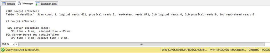
Figure 7-7. Benchmark with nonclustered index results
Figure 7-8 shows the execution plan for this query; it demonstrates the seek of the nonclustered index, followed by the key lookup to the clustered index.

Figure 7-8. Benchmark with nonclustered index execution plan
The next test is to alter the nonclustered index to include the ProductID and Quantity columns. This allows SQL Server to satisfy the entire query from the nonclustered index without accessing the base table at all. The script in Listing 7-8 makes this change to the index before rerunning the benchmark query.
The results in Figure 7-9 show that we have now brought the pages that need to be read from disk down to just two, and the execution time has reduced down to a mere 3ms.

Figure 7-9. Benchmark with nonclustered index, containing included columns results
The execution plan for this query is shown in Figure 7-10. As you can see, the Query Optimizer is able to perform a nonclustered index seek without performing a key lookup to the clustered index.
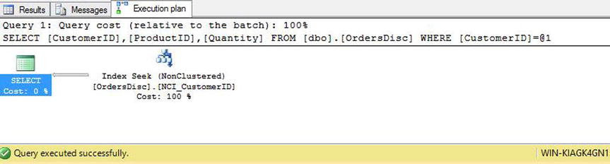
Figure 7-10. Benchmark with nonclustered index, containing included columns execution plan
When you create covering indexes, if you are only concerned with read performance, you want columns that are included in the WHERE clause, the JOIN clause, or the GROUP BY clause, or those that are involved in aggregations to be in the index key. You then want any columns that are returned with the query results but are not involved in these operations to be added as included columns. If any of the included columns are involved in the operations just mentioned, SQL Server may still be able to use the index, but only with a nonclustered index scan, as opposed to a nonclustered index seek. As you have seen in this section, a scan operation is less efficient than a seek operation, because it involves additional IO.
Because nonclustered indexes improve query performance but can have a negative impact on DML operations, it is sensible for DBAs to remove indexes that are infrequently used. You can identify indexes that are not being used by using the sys.dm_db_index_usage_stats DMV. The query in Listing 7-9 demonstrates using this DMV to find indexes that are infrequently used.
Indexes that have few scans or seeks, or indexes that have not been used for a significant amount of time, may be candidates for removal. This is even more important if the value for user_updates is high. This column increments every time the index needs to be modified because of DML statements in the base table.
![]() Caution There is no substitute for business knowledge, and just because you identify an index that has not been used for nearly a month does not necessarily mean that you should remove it. What if the index is used to support a time-critical business function that happens on a monthly basis? Always look deeper and never remove indexes without thought and consideration.
Caution There is no substitute for business knowledge, and just because you identify an index that has not been used for nearly a month does not necessarily mean that you should remove it. What if the index is used to support a time-critical business function that happens on a monthly basis? Always look deeper and never remove indexes without thought and consideration.
A filtered index is an index built on a subset of the data stored within a table, as opposed to one that is built on all of the data in the table. Because the indexes are smaller, they can lead to improved query performance and reduced storage cost. They also have the potential to cause less overhead for DML operations, since they only need to be updated if the DML operation affects the data within the index. For example, if an index was filtered on OrderDate >= '2014-01-01' AND OrderDate <= '2014-12-31' and subsequently updated all rows in the table where the OrderDate >= '2015-01-01', then the performance of the update would be the same as if the index did not exist.
Filtered indexes are constructed by using a WHERE clause on index creation. There are many things that you can do in the WHERE clause, such as filter on NULL or NOT NULL values; use equality and inequality operators, such as =, >, <, and IN; and use logical operators, such as AND and OR. There are also limitations, however. For example, you cannot use BETWEEN, CASE, or NOT IN. Also, you can only use simple predicates so, for example, using a date/time function is prohibited, so creating a rolling filter is not possible. You also cannot compare a column to other columns.
The statement in Listing 7-10 creates a filtered index on DelieveryDate, where the value is NULL. This allows you to make performance improvements on queries that are run to determine which orders are yet to have their delivery scheduled.
Indexes for Specialized Application
In addition to traditional B-tree indexes, SQL Server also provides several types of special indexes to help query performance against memory-optimized tables and against special data types within SQL Server, such as XML. The following sections discuss these special indexes. Although beyond the scope of this book, SQL Server also offers special indexes for geospatial data.
As you have seen, traditional indexes store rows of data on data pages. This is known as a rowstore. SQL Server also supports columnstore indexes. These indexes flip data around and use a page to store a column, as opposed to a set of rows. This is illustrated in Figure 7-11.

Figure 7-11. Colunstore index structure
A columnstore index slices the rows of a table into chunks of between 102,400 and 1,048,576 rows each. Each slice is called a rowgroup. Data in each rowgroup is then split down into columns and compressed using VertiPaq technology. Each column within a rowgroup is called a column segment.
Columnstore indexes offer several benefits over traditional indexes, given appropriate usage scenarios. First, because they are highly compressed, they can improve IO efficiency and reduce memory overhead. They can achieve such a high compression rate because data within a single column is often very similar between rows. Also, because a query is able to retrieve just the data pages of the column it requires, IO can again be reduced. This is helped even further by the fact that each column segment contains a header with metadata about the data within the segment. This means that SQL Server can access just the segments it needs, as opposed to the whole column. A new query execution mechanism has also been introduced to support columnstore indexes. It is called batch execution mode, and it allows data to be processed in chunks of 1000 rows, as opposed to on a row-by-row basis. This means that CPU usage is much more efficient. Columnstore indexes are not a magic bullet, however, and are designed to be optimal for data-warehouse style queries that perform read-only operations on very large tables. OLTP-style queries are not likely to see any benefit, and in some cases, may actually execute slower. SQL Server 2014 supports both clustered and nonclustered columnstore indexes, and these are discussed in the following sections.
Clustered columnstore indexes are new in SQL Server 2014 and cause the entire table to be stored in a columnstore format. There is no traditional rowstore storage for a table with a clustered columnstore index; however, new rows that are inserted into the table may temporarily be placed into a rowstore table, called a deltastore. This is to prevent the columnstore index from becoming fragmented and to enhance performance for DML operations. The diagram in Figure 7-12 illustrates this.

Figure 7-12. Clustered columnstore index with deltastores
The diagram shows that when data is inserted into a clustered columnstore index, SQL Server assesses the number of rows. If the number of rows is high enough to achieve a good compression rate, SQL Server treats them as a rowgroup or rowgroups and immediately compresses them and adds them to the columnstore index. If there are too few rows however, SQL Server inserts them into the internal deltastore structure. When you run a query against the table, the database engine seamlessly joins the structures together and returns the results as one. Once there are enough rows, the deltastore is marked as closed and a background process called the tuple compresses the rows into a rowgroup in the columnstore index.
There can be multiple deltastores for each clustered columnstore index. This is because, when SQL Server determines that an insert warrants using a deltastore, it attempts to access the existing deltastores. If all existing deltastores are locked, however, then a new one is created, instead of the query being forced to wait for a lock to be released.
When a row is deleted in a clustered columnstore index, then the row is only logically removed. The data still physically stays in the rowgroup until the next time the index is rebuilt. SQL Server maintains a B-tree structure of pointers to deleted rows in order to easily identify them. If the row being deleted is located in a deltastore, as opposed to the index itself, then it is immediately deleted, both logically and physically. When you update a row in a clustered columnstore index, then SQL Server marks the row as being logically deleted and inserts a new row into a deltastore, which contains the new values for the row.
You can create clustered columnstore indexes using a CREATE CLUSTERED COLUMNSTORE INDEX statement. Although a clustered columnstore index cannot coexist with traditional indexes, if a traditional clustered index already exists on the table, then you can create the clustered columnstore index using the DROP_EXISTING option. The script in Listing 7-11 copies the contents of the OrdersDisc table to a new table called OrdersColumnstore and then creates a clustered columnstore index on the table. When you create the index, you do not need to specify a key column; this is because all of the columns are added to column segments within the columnstore index. Your queries can then use the index to search on whichever column(s) it needs to satisfy the query. The clustered columnstore index is the only index on the table. You are not able to create traditional nonclustered indexes or a nonclustered columnstore index. Additionally, the table must not have primary key, foreign key, or unique constraints.
Not all data types are supported when you are using columnstore indexes. It is not possible to create a clustered columnstore index on tables that contain the following data types:
- TEXT
- NTEXT
- IMAGE
- VARCHAR(MAX)
- NVARCHAR(MAX)
- ROWVERSION
- SQL_VARIANT
- HIERARCHYID
- GEOGRAPHY
- GEOMETRY
- XML
Nonclustered Columnstore Indexes
Nonclustered columnstore indexes are not updateable. This means that if you create a nonclustered columnstore index on a table, that table becomes read only. The only way you can update or delete data from that table is to first drop or disable the columnstore index, and then re-create it once the DML process has completed. To insert data into a table with a nonclustered columnstore index, you must first either drop or disable the columnstore index or, alternatively, use partition switching to bring the data in. Partition switching is discussed in Chapter 6.
It is appropriate to use a nonclustered columnstore index instead of a clustered columnstore index when the table supports multiple workload profiles. In this scenario, the nonclustered columnstore index supports real-time analytics, whereas OLTP-style queries can make use of a traditional clustered index.
The statement in Listing 7-12 creates a nonclustered columnstore index on the FirstName, LastName, Balance, and CustomerID columns of the CustomersDisc table. You can see from our creation of this index that unlike clustered columnstore indexes, nonclustered columnstore indexes can coexist with traditional indexes and, in this case, we even cover some of the same columns.
Performance Considerations for Columnstore Indexes
In this section, we examine how different types of query perform when they are able to use a columnstore index, as opposed to a traditional index. We start with a simple SELECT * query, which uses a clustered index scan on the OrdersDisc table and a columnstore index scan on the OrdersColumnstore table, which of course, hold the same data. The script in Listing 7-13 runs this benchmark.
As you can see from the results in Figure 7-13, the clustered index actually performs better than the columnstore index.

Figure 7-13. Clustered index scan against columnstore index scan results
When we start to perform analysis on large datasets, we start to see the benefits of the columnstore index. The script in Listing 7-14 creates a nonclustered index to cover the CustomerID and NetAmount columns of the OrdersDisc table before it runs a benchmark test, which adds the data in the NetAmount column and groups by the CustomerID.
From the results in Figure 7-14, you can see that this time, the tables have turned and the columnstore index has outperformed the nonclustered index with an execution time over six times faster, which is pretty impressive.

Figure 7-14. Columnstore index against traditional nonclustered index for aggregation results
Figure 7-15 shows the execution plan for the two queries. We can see that the Query Optimizer is able to parallelize the query against the columnstore index. The query against the OrdersDisc table is run sequentially.

Figure 7-15. Execution plans
Also of interest, are the properties of the Columnstore Index Scan and the Hash Match operators, shown in Figure 7-16. Here we can see that SQL Server is able to use batch mode execution for both of these operators, which explains why the CPU time for the query against the columnstore index is 31ms as opposed to the 125ms for the query against the nonclustered index.

Figure 7-16. Execution plan properties
As we saw in Chapter 6, SQL Server provides two types of index for memory-optimized tables: nonclustered and nonclustered hash. Every memory-optimized table must have a minimum of one index and can support a maximum of eight. All in-memory indexes cover all columns in the table, because they use a memory pointer to link to the data row.
Indexes on memory-optimized tables must be created in the CREATE TABLE statement. There is no CREATE INDEX statement for in-memory indexes. Indexes built on memory-optimized tables are always stored in memory only and are never persisted to disk, regardless of your table’s durability setting. They are then re-created after the instance restarts. You do not need to worry about fragmentation of in-memory indexes, since they never have a disk-based structure.
In-memory Nonclustered Hash Indexes
A nonclustered hash index consists of an array of buckets. A hash function is run on each of the index keys, and then the hashed key values are placed into the buckets. The hashing algorithm used is deterministic, meaning that index keys with the same value always have the same hash value. This is important, because repeated hash values are always placed in the same hash bucket. When many keys are in the same hash bucket, performance of the index can degrade, because the whole chain of duplicates needs to be scanned to find the correct key. Therefore, if you are building a hash index on a nonunique column with many repeated keys, you should create the index with a much larger number of buckets. This should be in the realm of 20 to 100 times the number of distinct key values, as opposed to 2 times the number of unique keys that is usually recommended for unique indexes. Alternatively, using a nonclustered index on a nonunique column may offer a better solution. The second consequence of the hash function being deterministic is that different versions of the same row are always stored in the same hash bucket.
Even in the case of a unique index where only a single, current row version exits, the distribution of hashed values into buckets is not even, and if there are an equal number of buckets to unique key values, then approximately one third of the buckets is empty, one third contains a single value, and one third contains multiple values. When multiple values share a bucket, it is known as a hash collision, and a large number of hash collisions can lead to reduced performance. Hence the recommendation for the number of buckets in a unique index being twice the number of unique values expected in the table.
![]() Tip When you have a unique nonclustered hash index, in some cases, many unique values may hash to the same bucket. If you experience this, then increasing the number of buckets helps, in the same way that a nonunique index does.
Tip When you have a unique nonclustered hash index, in some cases, many unique values may hash to the same bucket. If you experience this, then increasing the number of buckets helps, in the same way that a nonunique index does.
As an example, if your table has one million rows, and the indexed column is unique, the optimum number of buckets, known as the BUCKET_COUNT is 2 million. If you know that you expect your table to grow to 2 million rows, however, then it may be prudent to create 4 million hash buckets. This number of buckets is low enough to not have an impact on memory. It also still allows for the expected increase in rows, without there being too few buckets, which would impair performance. An illustration of potential mappings between index values and hash buckets is illustrated in Figure 7-17.
![]() Tip The amount of memory used by a nonclustered hash index always remains static, since the number of buckets does not change.
Tip The amount of memory used by a nonclustered hash index always remains static, since the number of buckets does not change.

Figure 7-17. Mappings to a nonclustered hash index
Hash indexes are optimized for seek operations with the = predicate. For the seek operation, however, the full index key must be present in the predicate evaluation. If it is not, a full index scan is required. An index scan is also required if inequality predicates, such as < or > are used. Also, because the index is not ordered, the index cannot return the data in the sort order of the index key.
![]() Note You may remember that in Chapter 6, we witnessed superior performance from a disk-based table than from a memory-optimized table. This is explain by us using the > predicate in our query; this meant that although the disk-based index was able to perform an index seek, our memory-optimized hash index had to perform an index scan.
Note You may remember that in Chapter 6, we witnessed superior performance from a disk-based table than from a memory-optimized table. This is explain by us using the > predicate in our query; this meant that although the disk-based index was able to perform an index seek, our memory-optimized hash index had to perform an index scan.
Let’s now create a memory-optimized version of our OrdersDisc table, which includes a nonclustered hash index on the OrderID column, using the script in Listing 7-15. Initially, this row has 1 million rows, but we expect the number to grow to 2 million, so we use a BUCKET_COUNT of 4 million.
If we now wish to add an additional index to the table, we need to drop and re-create it. We already have data in the table, however, so we first need to create a temp table and copy the data in so that we can drop and re-create the memory-optimized table. The script in Listing 7-16 adds a nonclustered index to the OrderDate column.
We can examine the distribution of the values in our hash index by interrogating the sys.dm_db_xtp_hash_index_stats DMV. The query in Listing 7-17 demonstrates using this DMV to view the number of hash collisions and calculate the percentage of empty buckets.
From the results in Figure 7-18, we can see that for our hash index, 78 percent of the buckets are empty. The percentage is this high because we specified a large BUCKET_COUNT with table growth in mind. If the percentage was less than 33 percent, we would want to specify a higher number of buckets to avoid hash collisions. We can also see that we have an average chain length of 1, with a maximum chain length of 5. This is healthy. If the average chain count increases, then performance begins to tail off, since SQL Server has to scan multiple values to find the correct key. If the average chain length reaches 10 or higher, then the implication is that the key is nonunique and there are too many duplicate values in the key to make a hash index viable. At this point, we should either drop and re-create the table with a higher bucket count for the index or, ideally, look to implement a nonclustered index instead.

Figure 7-18. sys.dm_db_xtp_hash_index_stats results
In-memory Nonclustered Indexes
In-memory nonclustered indexes have a similar structure to a disk-based nonclustered index called a bw-tree. This structure uses a page-mapping table, as opposed to pointers, and is traversed using less than, as opposed to greater than, which is used when traversing disk-based indexes. The leaf level of the index is a singly linked list. Nonclustered indexes perform better than nonclustered hash indexes where a query uses inequality predicates, such as BETWEEN, >, or <. In-memory nonclustered indexes also perform better than a nonclustered hash index, where the = predicate is used, but not all of the columns in the key are used in the filter. Nonclustered indexes can also return the data in the sort order of the index key. Unlike disk-based indexes, however, these indexes cannot return the results in the reverse order of the index key.
Performance Considerations for In-memory Indexes
In Chapter 6, we saw that a memory-optimized table with a nonclustered hash index can offer significant performance gains over a disk-based table with a clustered index, as long as the correct query pattern is used. We also saw that results can be less favorable if inequality operators are used against a hash index. In this section, we evaluate the performance considerations when choosing between in-memory nonclustered indexes and nonclustered hash indexes.
The script in Listing 7-18 creates a new memory-optimized table, called OrdersMemNonClust. It then runs a query using an equality operator against the OrdersMemHash table, the OrdersMemNonClust table, and also the OrdersDisc table to generate a disk-based benchmark against a clustered index.
From the results in Figure 7-19, we can see that although the nonclustered index outperforms the disk-based table, by far the best results come from the nonclustered hash index, which takes less than a ms to complete.

Figure 7-19. Equality operator benchmark results
![]() Note Physical IO stats are of no use against memory-optimized tables.
Note Physical IO stats are of no use against memory-optimized tables.
For our next test, we use an inequality operator. The script in Listing 7-19 queries all three of our orders tables, but this time it uses the BETWEEN operator as opposed to the IN operator.
From the results in Figure 7-20, we can see that this time, the nonclustered index on the memory-optimized table offers by far the best performance. The nonclustered hash index is actually outperformed by the disk-based table. This is because a full scan of the nonclustered hash index is required, whereas an index seek is possible on the other two tables.

Figure 7-20. Inequality operator benchmark results
SQL Server allows you to store data in tables, in a native XML format, using the XML data type. Like other large object types, it can store up to 2GB per tuple. Although you can use standard operators such as = and LIKE against XML columns, you also have the option of using XQuery expressions. They can be rather inefficient unless you create XML indexes, however. XML indexes outperform full-text indexes for most queries against XML columns. SQL Server offers support for primary XML indexes and three types of secondary XML index; PATH, VALUE, and PROPERTY. Each of these indexes is discussed in the following sections.
A primary XML index is actually a multicolumn clustered index on an internal system table called the node table. This table stores a shredded representation of the XML objects within an XML column, along with the clustered index key of the base table. This means that a table must have a clustered index before a primary XML index can be created.
![]() Tip XML shredding is the process of extracting values from an XML document and using them to build a relational data set
Tip XML shredding is the process of extracting values from an XML document and using them to build a relational data set
The system table stores enough information that the scalar or XML subtrees that a query must have can be reconstructed from the index itself. This information includes the node ID and name, the tag name and URI, a tokenized version of the node’s data type, the first position of the node value in the document, pointers to the long node value and binary value, the nullability of the node, and the value of the base table’s clustered index key for the corresponding row.
Primary XML indexes can provide a performance improvement when a query needs to shred scalar values from an XML document(s) or return a subset of nodes from an XML document(s).
You can only create secondary XML indexes on XML columns that already have a primary XML index. Behind the scenes, secondary XML indexes are actually nonclustered indexes on the internal node table. Secondary XML indexes can improve query performance for queries that use specific types of XQuery processing.
A PATH secondary XML index is built on the NodeID and Value columns of the node table. This type of index offers performance improvements to queries that use path expressions, such as the exists() XQuery method. A VALUE secondary XML index is the reverse of this, and it is built on the VALUE and NodeID columns. This type of index offers gains to queries that search for values without knowing the name of the XML element or attribute that contains the value the query is searching for. Finally, a PROPERTY secondary XML index is built on the clustered index key of the base table, the NodeID and the Value columns of the nodes table. This type of index performs very well if the query is trying to retrieve nodes from multiple rows of the base table.
Performance Considerations for XML Indexes
In order to discuss the performance considerations for XML indexes, we first need to create and populate a table that has an XML column. The script in Listing 7-20 creates a table with an XML column called OrderSummary. Next, it populates this table by using a FOR XML query against the OrdersDisc and CustomersDisc tables within our Chapter7 database, and it creates a primary XML index on the column. It then runs a query against the table in order to benchmark the results with just a primary XML index.
![]() Tip Details of the FOR XML query can be found at msdn.microsoft.com/en-GB/library/ms178107(v=sql.120).aspx and details of the XQuery exist method can be found at msdn.microsoft.com/en-us/library/ms189869.aspx.
Tip Details of the FOR XML query can be found at msdn.microsoft.com/en-GB/library/ms178107(v=sql.120).aspx and details of the XQuery exist method can be found at msdn.microsoft.com/en-us/library/ms189869.aspx.
From the results in Figure 7-21, we can see that with just a primary XML index on the column, the query took over four seconds to complete.

Figure 7-21. Benchmark primary XML index results
The next test involves adding a secondary XML index. Because we are running a query with the exist() XQuery method, the most suitable secondary index to create is a PATH index. The script in Listing 7-21 creates a PATH index and then reruns the benchmark query.
The results in Figure 7-22 show that adding the PATH secondary XML index reduces the query time by over 800ms.

Figure 7-22. PATH index benchmark results
Administering XML Indexes
As you can see from the code examples in the previous section, primary XML indexes are created using the CREATE PRIMARY XML INDEX syntax. You use the ON clause to specify the name of the table and column as you would for a traditional index.
When we create the PATH secondary XML index in the preceding code samples, we use the CREATE XML INDEX syntax. We then use the USING XML INDEX line to specify the name of the primary XML index on which the secondary index is built. The final line of the statement uses the FOR clause to specify that we want it to be built as a PATH index. Alternatively, we could have stated FOR PROPERTY or FOR VALUE, to build PROPERTY or VALUE secondary XML indexes instead.
XML indexes can be dropped with the DROP INDEX statement, specifying the table and index name to be removed. Dropping a primary XML index also drops any secondary XML indexes that are associated with it.
Maintaining Indexes
Once indexes have been created, a DBAs work is not complete. Indexes need to be maintained on an ongoing basis. The following sections discuss considerations for index maintenance.
Disk-based indexes are subject to fragmentation. Two forms of fragmentation can occur in B-trees: internal fragmentation and external fragmentation. Internal fragmentation refers to pages having lots of free space. If pages have lots of free space, then SQL Server needs to read more pages than is necessary to return all of the required rows for a query. External fragmentation refers to the pages of the index becoming out of physical order. This can reduce performance, since the data cannot be read sequentially from disk.
For example, imagine that you have a table with 1 million rows of data, and that all of these data rows fit into 5000 pages when the data pages are 100-percent full. This means that SQL Server needs to read just over 39MB of data in order to scan the entire table (8KB * 5000). If the pages of the table are only 50 percent full, however, this increases the number of pages in use to 10,000, which also increases the amount of data that needs to be read to 78MB. This is internal fragmentation.
Internal fragmentation can occur naturally when DELETE statements are issued and when DML statements occur, such as when a key value that is not ever-increasing is inserted. This is because SQL Server may respond to this situation by performing a page split. A page split creates a new page, moves half of the data from the existing page to the new page, and leaves the other half on the existing page, thus creating 50 percent free space on both pages. They can also occur artificially, however, through the misuse of the FILLFACTOR and PAD_INDEX settings.
FILLFACTOR controls how much free space is left on each leaf level page of an index when it is created or rebuilt. By default, the FILLFACTOR is set to 0, which means that it leaves enough space on the page for exactly one row. In some cases, however, when a high number of page splits is occurring due to DML operations, a DBA may be able to reduce fragmentation by altering the FILLFACTOR. Setting a FILLFACTOR of 80, for example, leaves 20-percent free space in the page, meaning that new rows can be added to the page without page splits occurring. Many DBAs change the FILLFACTOR when they are not required to, however, which automatically causes internal fragmentation as soon as the index is built. PAD_INDEX can be applied only when FILLFACTOR is used, and it applies the same percentage of free space to the intermediate levels of the B-tree.
External fragmentation is also caused by page splits and refers to the logical order of pages, as ordered by the index key, being out of sequence when compared to the physical order of pages on disk. External fragmentation makes it so SQL Server is less able to perform scan operations using a sequential read, because the head needs to move backward and forward over the disk to locate the pages within the file.
![]() Note This is not the same as fragmentation at the file system level where a data file can be split over multiple, unordered disk sectors.
Note This is not the same as fragmentation at the file system level where a data file can be split over multiple, unordered disk sectors.
You can identify fragmentation of indexes by using the sys.dm_db_index_physical_stats DMF. This function accepts the parameters listed in Table 7-2.
Table 7-2. sys.dm_db_index_physical_stats Parameters
|
Parameter |
Description |
|---|---|
|
Database_ID |
The ID of the database that you want to run the function against. If you do not know it, you can pass in DB_ID('MyDatabase') where MyDatabase is the name of your database. |
|
Object_ID |
The Object ID of the table that you want to run the function against. If you do not know it, pass in OBJECT_ID('MyTable') where MyTable is the name of your table. Pass in NULL to run the function against all tables in the database. |
|
Index_ID |
The index ID of the index you want to run the function against. This is always 1 for a clustered index. Pass in NULL to run the function against all indexes on the table. |
|
Partition_Number |
The ID of the partition that you want to run the function against. Pass in NULL if you want to run the function against all partitions, or if the table is not partitioned. |
|
Mode |
Choose LIMITED, SAMPLED, or DETAILED. LIMITED only scans the non–leaf levels of an index. SAMPLED scans 1 percent of pages in the table, unless the table has 10,000 pages or less, in which case DETAILED mode is used. DETAILED mode scans 100 percent of the pages in the table. For very large tables, SAMPLED is often preferred due to the length of time it can take to return data in DETAILED mode. |
Listing 7-22 demonstrates how we can use sys.dm_db_index_physical_stats to check the fragmentation levels of our OrdersDisc table.
The output of this query is shown in Figure 7-23. You can see that one row is returned for every level of each B-tree. If the table was partitioned, this would also be broken down by partition. The index_level column indicates which level of the B-tree is represented by the row. Level 0 implies the leaf level of the B-tree, whereas Level 1 is either the lowest intermediate level or the root level if no intermediate levels exist, and so on, with the highest number always reflecting the root node. The avg_fragmentation_in_percent column tells us how much external fragmentation is present. We want this value to be as close to zero as possible. The avg_page_space_used_in_percent tells us how much internal fragmentation is present, so we want this value to be as close to 100 as possible. The Internal_Frag_With_FillFactor_Offset column also tells us how much internal fragmentation is present, but this time, it applies an offset to allow for the fill factor that has been applied to the index. The fragment_count column indicates how many chucks of continuous pages exist for the index level, so we want this value to be as low as possible. The avg_fragment_size_in_pages column tells the average size of each fragment, so obviously this number should also be as high as possible.

Figure 7-23. sys.dm_db_index_physical_stats results
You can remove fragmentation by either reorganizing or rebuilding an index. When you reorganize an index, SQL Server reorganizes the data within the leaf level of the index. It looks to see if there is free space on a page that it can use. If there is, then it moves rows from the next page, onto this page. If there are empty pages at the end of this process, then they are removed. SQL Server only fills pages to the level of the FillFactor specified. Once this is complete, the data within the leaf level pages is shuffled so that their physical order is a closer match to their logical, key order. Reorganizing an index is always an ONLINE operation, meaning that the index can still be used by other processes while the operation is in progress. Where it is always an ONLINE operation, it will fail if the ALLOW_PAGE_LOCKS option is turned off. The process of reorganizing an index is suitable for removing internal fragmentation and low levels of external fragmentation of 30 percent or less. However, it makes no guarantees, even with this usage profile, that there will not be fragmentation left after the operation completes.
The script in Listing 7-23 demonstrates how we can reorganize the NCI_CustomerID_NetAmount index on the OrdersDisc table.
When you rebuild an index, the existing index is dropped and then completely rebuilt. This, by definition, removes internal and external fragmentation, since the index is built from scratch. It is important to note, however, that you are still not guaranteed to be 100-percent fragmentation free after this operation. This is because SQL Server assigns different chunks of the index to each CPU core that is involved in the rebuild. Each CPU core should build its own section in the perfect sequence, but when the pieces are synchronized, there may be a small amount of fragmentation. You can minimize this issue by specifying MAXDOP = 1. Even when you set this option, you may still encounter fragmentation in some cases. For example, if ALLOW_PAGES_LOCKS is configured as OFF, then the workers share the allocation cache, which can cause fragmentation. Additionally, when you set MAXDOP = 1 it is at the expense of the time it takes to rebuild the index.
You can rebuild an index by performing either an ONLINE or OFFLINE operation. If you choose to rebuild the index as an ONLINE operation, then the original version of the index is still accessible, whilst the operation takes place. The ONLINE operation comes at the expense of both time and resource utilization. You need to enable ALLOW_PAGE_LOCKS to make your ONLINE rebuild successful.
The script in Listing 7-24 demonstrates how we can rebuild the NCI_CustomerID index on the OrdersDisc table. Because we have not specified ONLINE = ON, it uses the default setting of ONLINE = OFF, and the index is locked for the entire operation. Because we specify MAXDOP = 1, the operation is slower, but has no fragmentation.
If you create a maintenance plan to rebuild or reorganize indexes, then all indexes within the specified database are rebuilt, regardless of whether they need to be—this can be time consuming and eat resources. You can resolve this issue by using the sys.dm_db_index_physical_stats DMF to create an intelligent script that you can run from SQL Server Agent and use to reorganize or rebuild only those indexes that require it. This is discussed in more detail in Chapter 17.
![]() Tip There is a myth that using SSDs removes the issue of index fragmentation. This is not correct. Although SSDs reduce the performance impact of out-of-order pages, they do not remove it. They also have no impact on internal fragmentation.
Tip There is a myth that using SSDs removes the issue of index fragmentation. This is not correct. Although SSDs reduce the performance impact of out-of-order pages, they do not remove it. They also have no impact on internal fragmentation.
When you run queries, the Database Engine keeps track of any indexes that it would like to use when building a plan to aid your query performance. When you view an execution plan in SSMS, you are provided with advice on missing indexes, but the data is also available later through DMVs.
![]() Tip Because the suggestions are based on a single plan, you should review them as opposed to implementing them blindly.
Tip Because the suggestions are based on a single plan, you should review them as opposed to implementing them blindly.
In order to demonstrate this functionality, we drop all of the nonclustered indexes on the OrdersDisc and CustomersDisc tables. We can then execute the query in Listing 7-25 and choose to include the actual execution plan.
![]() Tip You can see missing index information by viewing the estimated query plan.
Tip You can see missing index information by viewing the estimated query plan.
Once we have run this query, we can examine the execution plan and see what it tells us. The execution plan for this query is shown in Figure 7-24.

Figure 7-24. Execution plan showing missing indexes
At the top of the execution plan in Figure 7-24, you can see that SQL Server is recommending that we create an index on the CustomerID column of the OrdersDisc table and include the NetAmount column at the leaf level. We are also advised that this should provide a 95-percent performance improvement to the query.
As mentioned, SQL Server also makes this information available through DMVs. The sys.dm_db_missing_index_details DMV joins to the sys.dm_db_missing_index_group_stats through the intermediate DMV sys.dm_db_missing_index_groups, which avoids a many-to-many relationship. The script in Listing 7-26 demonstrates how we can use these DMVs to return details on missing indexes.
The results of this query are shown in Figure 7-25. They show the following: the name of the table with the missing index; the column(s) that SQL Server recommends should form the index key; the columns that SQL Server recommends should be added as included columns at the leaf level of the B-tree; the number of times that queries that would have benefited from the index have been compiled; how many seeks would have been performed against the index, if it existed; the number of times that the index has been scanned if it existed; the average cost that would have been saved by using the index; and the average percentage cost that would have been saved by using the index. In our case, we can see that the query would have been 95 percent less expensive if the index existed when we ran our query.

Figure 7-25. Missing index results
As mentioned in Chapter 6, it is possible to partition indexes as well as tables. A clustered index always shares the same partition scheme as the underlying table, because the leaf level of the clustered index is made up of the actual data pages of the table. Nonclustered indexes, on the other hand, can either be aligned with the table or not. Indexes are aligned if they share the same partition scheme or if they are created on an identical partition scheme.
In most cases, it is good practice to align nonclustered indexes with the base table, but on occasion, you may wish to deviate from this strategy. For example, if the base table is not partitioned, you can still partition an index for performance. Also, if you index key is unique and does not contain the partitioning key, then it needs to be unaligned. There is also an opportunity to gain a performance boost from unaligned nonclustered indexes if the table is involved in collated joins with other tables on different columns.
You can create a partitioned index by using the ON clause to specify the partition scheme in the same way that you create a partitioned table. If the index already exists, you can rebuild it, specifying the partition scheme in the ON clause. The script in Listing 7-27 creates a partition function and a partition scheme. It then rebuilds the clustered index of the OrdersDisc table to move it to the new partition scheme. Finally, it creates a new nonclustered index, which is partition aligned with the table.
![]() Tip Before running the script, change the name of the primary key to match your own.
Tip Before running the script, change the name of the primary key to match your own.
When you rebuild an index, you can also specify that only a certain partition is rebuilt. The example in Listing 7-28 rebuilds only Partition 1 of the NCI_Part_CustID index.
SQL Server maintains statistics regarding the distribution of data within a column or set of columns. These columns can either be within a table or a nonclustered index. When the statistics are built on a set of columns, then they also include correlation statistics between the distributions of values in those columns. The Query Optimizer can then use these statistics to build efficient query plans based on the number of rows that it expects a query to return. A lack of statistics can lead to inefficient plans being generated. For example, the Query Optimizer may decide to perform an index scan when a seek operation would be more efficient.
You can allow SQL Server to manage statistics automatically. A database level option called AUTO_CREATE_STATISTICS automatically generates single column statistics, where SQL Server believes better cardinality estimates will help query performance. There are limitations to this however. For example, filtered statistics or multicolumn statistics cannot be created automatically.
![]() Tip The only exception to this is when an index is created. When you create an index, statistics are always generated, even multicolumn statistics, to cover the index key. It also includes filtered statistics on filtered indexes. This is regardless of the AUTO_CREATE_STATS setting.
Tip The only exception to this is when an index is created. When you create an index, statistics are always generated, even multicolumn statistics, to cover the index key. It also includes filtered statistics on filtered indexes. This is regardless of the AUTO_CREATE_STATS setting.
Auto Create Incremental Stats causes statistics on partitioned tables to be automatically created on a per-partition basis, as opposed to being generated for the whole table. This can reduce contention by stopping a scan of the full table from being required. This is a new feature in SQL Server 2014.
Statistics become out of date as DML operations are performed against a table. The database level option, AUTO_UPDATE_STATISTICS, rebuilds statistics when they become outdated. The rules in Table 7-3 are used to determine if statistics are out of date.
Table 7-3. Statistics Update Algorithms
|
No of Rows in Table |
Rule |
|---|---|
|
0 |
Table has greater than 0 rows. |
|
<= 500 |
500 or more values in the first column of the statistics object have changed. |
|
> 500 |
500 + 20 percent or more values in the first column of the statistics object have changed. |
|
Partitioned table with INCREMENTAL statistics |
20 percent or more of values in the first column of the statistics object for a specific partition have changed. |
The AUTO_UPDATE_STATISTICS process is very useful and it is normally a good idea to use it. An issue can arise, however, because the process is synchronous and blocking. Therefore, if a query is run, SQL Server checks to see if the statistics need to be updated. If they do, SQL Server updates them, but this blocks the query and any other queries that require the same statistics, until the operation completes. During times of high read/write load, such as an ETL process against very large tables, this can cause performance problems. The workaround for this is another database level option, called AUTO_UPDATE_STATISTICS_ASYNC. Even when this option is turned on, it only takes effect if AUTO_UPDATE_STATISTICS is also turned on. When enabled, AUTO_UPDATE_STATS_ASYNC forces the update of the statistics object to run as an asynchronous background process. This means that the query that caused it to run and other queries are not blocked. The tradeoff, however, is that these queries do not benefit from the updated statistics.
The options mentioned earlier can be configured on the Options page of the Database Properties dialog box. This is illustrated in Figure 7-26.

Figure 7-26. The Options page
Alternatively, you can configure them using ALTER DATABASE commands, as demonstrated in Listing 7-29.
Filtered statistics allow you to create statistics on a subset of data within a column through the use of a WHERE clause in the statistic creation. This allows the Query Optimizer to generate an even better plan, since the statistics only contain the distribution of values within the well-defined subset of data. For example, if we create filtered statistics on the NetAmount column of our OrdersDisc table filtered by OrderDate being greater than 1 Jan 2014, then the statistics will not include rows that contain old orders, allowing us to search for large, recent orders more efficiently.
Incremental Statistics
Incremental statistics can help reduce table scans caused by statistics updates on large partitioned tables. When enabled, statistics are created and updated on a per-partition basis, as opposed to globally, for the entire table. This can significantly reduce the amount of time you need to update statistics on large partitioned tables, since partitions where the statistics are not outdated are not touched, therefore reducing unnecessary overhead.
Incremental statistics are not supported in all scenarios, however. A warning is generated and the setting is ignored, if the option is used with the following types of statistics:
- Statistics on views
- Statistics on XML columns
- Statistics on Geography or Geometry columns
- Statistics on filtered indexes
- Statistics for indexes that are not partition aligned
Additionally, you cannot use incremental statistics on read-only databases or on databases that are participating in an AlwaysOn Availability Group as a readable secondary replica.
Managing Statistics
In addition to being automatically created and updated by SQL Server, you can also create and update statistics manually using the CREATE STATISTICS statement. If you wish to create filtered statistics, add a WHERE clause at the end of the statement. The script in Listing 7-30 creates a multicolumn statistic on the FirstName and LastName columns of the CustomersDisc table. It then creates a filtered statistic on the NetAmount column of the OrdersDisc table, built only on rows where the OrderDate is greater than 1st Jan 2014.
When creating statistics, you can use the options detailed in Table 7-4.
Table 7-4. Creating Statistics Options
|
Option |
Description |
|---|---|
|
FULLSCAN |
Creates the statistic object on a sample of 100 percent of rows in the table. This option creates the most accurate statistics but takes the longest time to generate. |
|
SAMPLE |
Specifies the number of rows or percentage of rows you need to use to build the statistic object. The larger the sample, the more accurate the statistic, but the longer it takes to generate. Specifying 0 creates the statistic but does not populate it. |
|
NORECOMPUTE |
Excludes the statistic object from being automatically updated with AUTO_UPDATE_STATISTICS. |
|
INCREMENTAL |
Overrides the database-level setting for incremental statistics. |
Individual statistics, or all statistics on an individual table, can be updated by using the UPDATE STATISTICS statement. The script in Listing 7-31 first updates the Stat_NetAmount_Filter_OrderDate statistics object that we created on the OrdersDisc table and then updates all statistics on the CustomersDisc table.
When using UPDATE STATISTICS, in addition to the options specified in Table 7-4 for creating statistics, which are all valid when updating statistics, the options detailed in Table 7-5 are also available.
Table 7-5. Updating Statistics Options
|
Option |
Description |
|---|---|
|
RESAMPLE |
Uses the most recent sample rate to update the statistics. |
|
ON PARTITIONS |
Causes statistics to be generated for the partitions listed and then merges them together to create global statistics. |
|
ALL | COLUMNS | INDEX |
Specifies if statistics should be updated for just columns, just indexes, or both. The default is ALL. |
You can also update statistics for an entire database by using the sp_updatestats system stored procedure. This procedure updates out-of-date statistics on disk-based tables and all statistics on memory-optimized tables regardless of whether they are out of date or not. Listing 7-32 demonstrates this system stored procedure’s usage to update statistics in the Chapter7 database. Passing in the RESAMPLE parameter causes the most recent sample rate to be used. Omitting this parameter causes the default sample rate to be used.
![]() Note Updating statistics causes queries that use those statistics to be recompiled the next time they run. The only time this is not the case is if there is only one possible plan for the tables and indexes referenced. For example, SELECT * FROM MyTable always performs a clustered index scan, assuming that the table has a clustered index.
Note Updating statistics causes queries that use those statistics to be recompiled the next time they run. The only time this is not the case is if there is only one possible plan for the tables and indexes referenced. For example, SELECT * FROM MyTable always performs a clustered index scan, assuming that the table has a clustered index.
Summary
A table that does not have a clustered index is called a heap and the data pages of the table are stored in no particular order. Clustered indexes build a B-tree structure, based on the clustered index key, and cause the data within the table to be ordered by that key. There can only ever be one clustered index on a table because the leaf level of the clustered index is the actual data pages of the table, and the pages can only be physically ordered in one way. The natural choice of key for a clustered index is the primary key of the table and, by default, SQL Server automatically creates a clustered index on the primary key. There are situations, however, when you may choose to use a different column as the clustered index key. This is usually when the primary key of the table is very wide, is updateable, or is not ever-increasing.
Nonclustered indexes are also B-tree structures built on other columns within a table. The difference is that the leaf level of a nonclustered index contains pointers to the data pages of the table, as opposed to the data pages themselves. Because a nonclustered index does not order the actual data pages of a table, you can create multiple nonclustered indexes. These can improve query performance when you create them on columns that are used in WHERE, JOIN, and GROUP BY clauses. You can also include other columns at the leaf level of the B-tree of a nonclustered index in order to cover a query. A query is covered by a nonclustered index, when you do not need to read the data from the underlying table. You can also filter a nonclustered index by adding a WHERE clause to the definition. This allows for improved query performance for queries that use a well-defined subset of data.
Columnstore indexes compress data and store each column in a distinct set of pages. This can significantly improve the performance of data-warehouse–style queries, which perform analysis on large data sets, since only the required columns need to be accessed, as opposed to the entire row. Each column is also split into segments, with each segment containing a header with metadata about the data, in order to further improve performance by allowing SQL Server to only access the relevant segments, in order to satisfy a query. Nonclustered columnstore indexes are not updatable, meaning that you must disable or drop the index before DML statements can occur on the base table. You can, on the other hand, update clustered columnstore indexes. Clustered columnstore indexes are a new feature of SQL Server 2014.
You can create two types of index on memory-optimized tables: nonclustered indexes and nonclustered hash indexes. Nonclustered hash indexes are very efficient for point lookups, but they can be much less efficient when you must perform a range scan. Nonclustered indexes perform better for operations such as inequality comparisons, and they are also able to return the data in the sort order of the index key.
You can create XML indexes on columns with the XML data type in order to improve query performance. You can only create a primary XML index if a clustered index already exists on the table and it works by creating a clustered index on an internal nodes table, which stores metadata and shredded node values. When you then need XML fragments or scalar values, you can use this data to reconstruct the nodes. Secondary XML indexes can further improve performance by creating nonclustered indexes on the internal nodes table. A PATH index can improve performance for XQuery methods such as exists(). A VALUE index can improve performance for XQuery expressions that search for values without knowing the name of the element. A PROPERTY index improves performance for queries that return nodes from multiple rows within a table, since a PROPERTY includes the clustered index key.
Indexes need to be maintained over time. They become fragmented due to DML statements causing page splits and can be reorganized or rebuilt to reduce or remove fragmentation. When pages become out of sequence, this is known as external fragmentation, and when pages have lots of free space, this is known as internal fragmentation. SQL Server stores metadata regarding index fragmentation and can display this through a DMF called sys.dm_db_index_physical_stats. SQL Server also maintains information on indexes that it regards as missing. A missing index is an index that does not exist in the database but would improve query performance if it were created. DBAs can use this data help them improve their indexing strategies.
SQL Server maintains statistics about the distribution of values within a column or set of columns to help improve the quality of query plans. Without good-quality statistics, SQL Server may make the wrong choice about which index or index operator to use in order to satisfy a query. For example, it may choose to perform an index scan when an index seek would have been more appropriate. You can update statistics manually or automatically, but either way causes queries to be recompiled. SQL Server 2014 also introduces incremental statistics, which allow statistics to be created on a per-partition basis, as opposed to globally for an entire table.