
![]()
High Availability and Disaster Recovery Concepts
In today’s 24×7 environments that are running mission critical applications, businesses rely heavily on the availability of their data. Although servers and their software are generally reliable, there is always the risk of a hardware failure or a software bug, each of which could bring a server down. To mitigate these risks, business-critical applications often rely on redundant hardware to provide fault tolerance. If the primary system fails, then the application can automatically fail over to the redundant system. This is the underlying principle of high availability (HA).
Even with the implementation of HA technologies, there is always a small risk of an event that causes the application to become unavailable. This could be due to a major incident, such as the loss of a data center, due to a natural disaster, or due to an act of terrorism. It could also be caused by data corruption or human error, resulting in the application’s data becoming lost or damaged beyond repair.
In these situations, some applications may rely on restoring the latest backup to recover as much data as possible. However, more critical applications may require a redundant server to hold a synchronized copy of the data in a secondary location. This is the underpinning concept of disaster recovery (DR). This chapter discusses the concepts behind HA and DR before providing an overview of the technologies that are available to implement these concepts.
Availability Concepts
In order to analyze the HA and DR requirements of an application and implement the most appropriate solution, you need to understand various concepts. We discuss these concepts in the following sections.
The amount of time that a solution is available to end users is known as the level of availability, or uptime. To provide a true picture of uptime, a company should measure the availability of a solution from a user’s desktop. In other words, even if your SQL Server has been running uninterrupted for over a month, users may still experience outages to their solution caused by other factors. These factors can include network outages or an application server failure.
In some instances, however, you have no choice but to measure the level of availability at the SQL Server level. This may be because you lack holistic monitoring tools within the Enterprise. Most often, however, the requirement to measure the level of availability at the instance level is political, as opposed to technical. In the IT industry, it has become a trend to outsource the management of data centers to third-party providers. In such cases, the provider responsible for managing the SQL servers may not necessarily be the provider responsible for the network or application servers. In this scenario, you need to monitor uptime at the SQL Server level to accurately judge the performance of the service provider.
The level of availability is measured as a percentage of the time that the application or server is available. Companies often strive to achieve 99 percent, 99.9 percent, 99.99 percent, or 99.999 percent availability. As a result, the level of availability is often referred to in 9s. For example, five 9s of availability means 99.999 percent uptime and three 9s means 99.9 percent uptime.
Table 11-1 details the amount of acceptable downtime per week, per month, and per year for each level of availability.

To calculate other levels of availability, you can use the script in Listing 11-1. Before running this script, replace the value of @Uptime to represent the level of uptime that you wish to calculate. You should also replace the value of @UptimeInterval to reflect uptime per week, month, or year.
Service-Level Agreements and Service-Level Objectives
When a third-party provider is responsible for managing servers, the contract usually includes service-level agreements(SLAs). These SLAs define many parameters, including how much downtime is acceptable, the maximum length of time a server can be down in the event of failure, and how much data loss is acceptable if failure occurs. Normally, there are financial penalties for the provider if these SLAs are not met.
In the event that servers are managed in-house, DBAs still have the concept of customers. These are usually the end users of the application, with the primary contact being the business owner. An application’s business owner is the stakeholder within the business who commissioned the application and who is responsible for signing off on funding enhancements, among other things.
In an in-house scenario, it is still possible to define SLAs, and in such a case, the IT Infrastructure or Platform departments may be liable for charge-back to the business teams if these SLAs are not being met. However, in internal scenarios, it is much more common for IT departments to negotiate service-level objectives (SLOs) with the business teams, as opposed to SLAs. SLOs are very similar in nature to SLAs, but their use implies that the business do not impose financial penalties on the IT department in the event that they are not met.
It is important to remember that downtime is not only caused by failure, but also by proactive maintenance. For example, if you need to patch the operating system, or SQL Server itself, with the latest service pack, then you must have some downtime during installation.
Depending on the upgrade you are applying, the downtime in such a scenario could be substantial—several hours for a stand-alone server. In this situation, high availability is essential for many business-critical applications—not to protect against unplanned downtime, but to avoid prolonged outages during planned maintenance.
Recovery Point Objective and Recovery Time Objective
The recovery point objective (RPO) of an application indicates how much data loss is acceptable in the event of a failure. For a data warehouse that supports a reporting application, for example, this may be an extended period, such as 24 hours, given that it may only be updated once per day by an ETL process and all other activity is read-only reporting. For highly transactional systems, however, such as an OLTP database supporting trading platforms or web applications, the RPO will be zero. An RPO of zero means that no data loss is acceptable.
Applications may have different RPOs for high availability and for disaster recovery. For example, for reasons of cost or application performance, an RPO of zero may be required for a failover within the site. If the same application fails over to a DR data center, however, five or ten minutes of data loss may be acceptable. This is because of technology differences used to implement intra-site availability and inter-site recovery.
The recovery time objective (RTO) for an application specifies the maximum amount of time an application can be down before recovery is complete and users can reconnect. When calculating the achievable RTO for an application, you need to consider many aspects. For example, it may take less than a minute for a cluster to fail over from one node to another and for the SQL Server service to come back up; however it may take far longer for the databases to recover. The time it takes for databases to recover depends on many factors, including the size of the databases, the quantity of databases within an instance, and how many transactions were in-flight when the failover occurred. This is because all noncommitted transactions need to be rolled back.
Just like RPO, it is common for there to be different RTOs depending on whether you have an intra-site or inter-site failover. Again, this is primarily due to differences in technologies, but it also factors in the amount of time you need to bring up the entire estate in the DR data center if the primary data center is lost.
The RPO and RTO of an application may also vary in the event of data corruption. Depending on the nature of the corruption and the HA/DR technologies that have been implemented, data corruption may result in you needing to restore a database from a backup.
If you must restore a database, the worst-case scenario is that the achievable point of recovery may be the time of the last backup. This means that you must factor a hard business requirement for a specific RPO into you backup strategy. (Backups are discussed fully in Chapter 15.) If only part of the database is corrupt, however, you may be able to salvage some data from the live database and restore only the corrupt data from the restored database.
Data corruption is also likely to have an impact on the RTO. One of the biggest influencing factors is if backups are stored locally on the server, or if you need to retrieve them from tape. Retrieving backup files from tape, or even from off-site locations, is likely to add significant time to the recovery process.
Another influencing factor is what caused the corruption. If it is caused by a faulty IO subsystem, then you may need to factor in time for the Windows administrators to run the check disk command (CHKDSK) against the volume and potentially more time for disks to be replaced. If the corruption is caused by a user accidently truncating a table or deleting a data file, however, then this is not of concern.
If you ask any business owners how much downtime is acceptable for their applications and how much data loss is acceptable, the answers invariably come back as zero and zero, respectively. Of course, it is never possible to guarantee zero downtime, and once you begin to explain the costs associated with the different levels of availability, it starts to get easier to negotiate a mutually acceptable level of service.
The key factor in deciding how many 9s you should try to achieve is the cost of downtime. Two categories of cost are associated with downtime: tangible costs and intangible costs. Tangible costs are usually fairly straightforward to calculate. Let’s use a sales application as an example. In this case, the most obvious tangible cost is lost revenue because the sales staff cannot take orders. Intangible costs are more difficult to quantify but can be far more expensive. For example, if a customer is unable to place an order with your company, they may place their order with a rival company and never return. Other intangible costs can include loss of staff morale, which leads to higher staff turnover, or even loss of company reputation. Because intangible costs, by their very nature, can only be estimated, the industry rule of thumb is to multiply the tangible costs by three and use this figure to represent your intangible costs.
Once you have an hourly figure for the total cost of downtime for your application, you can scale this figure out, across the predicted lifecycle of your application, and compare the costs of implementing different availability levels. For example, imagine that you calculate that your total cost of downtime is $2,000/hour and the predicted lifecycle of your application is three years. Table 11-2 illustrates the cost of downtime for your application, comparing the costs that you have calculated for implementing each level of availability, after you have factored in hardware, licenses, power, cabling, additional storage, and additional supporting equipment, such as new racks, administrative costs, and so on. This is known as the total cost of ownership (TCO) of a solution.
Table 11-2. Cost of Downtime
|
Level of Availability |
Cost of Downtime (Three Years) |
Cost of Availability Solution |
|---|---|---|
|
99% |
$525,600 |
$108,000 |
|
99.9% |
$52,560 |
$224,000 |
|
99.99% |
$5,256 |
$462,000 |
|
99.999% |
$526 |
$910,000 |
In this table, you can see that implementing five 9s of availability saves $525,474 over a two-9s solution, but the cost of implementing the solution is an additional $802,000, meaning that it is not economical to implement. Four 9s of availability saves $520,334 over a two-9s solution and only costs an additional $354,000 to implement. Therefore, for this particular application, a four-9s solution is the most appropriate level of service to design for.
Classification of Standby Servers
There are three classes of standby solution. You can implement each using different technologies, although you can use some technologies to implement multiple classes of standby server. Table 11-3 outlines the different classes of standby that you can implement.
Table 11-3. Standby Classifications
|
Class |
Description |
Example Technologies |
|---|---|---|
|
Hot |
A synchronized solution where failover can occur automatically or manually. Often used for high availability. |
|
|
Warm |
A synchronized solution where failover can only occur manually. Often used for disaster recovery. |
|
|
Cold |
An unsynchronized solution where failover can only occur manually. This is only suitable for read-only data, which is never modified. |
- |
![]() Note Cold standby does not show an example technology because no synchronization is required and, thus, no technology implementation is required.
Note Cold standby does not show an example technology because no synchronization is required and, thus, no technology implementation is required.
High Availability and Recovery Technologies
SQL Server provides a full suite of technologies for implementing high availability and disaster recovery. The following sections provide an overview of these technologies and discuss their most appropriate uses.
A Windows cluster is a technology for providing high availability in which a group of up to 64 servers works together to provide redundancy. An AlwaysOn Failover Clustered Instance (FCI) is an instance of SQL Server that spans the servers within this group. If one of the servers within this group fails, another server takes ownership of the instance. Its most appropriate usage is for high availability scenarios where the databases are large or have high write profiles. This is because clustering relies on shared storage, meaning the data is only written to disk once. With SQL Server–level HA technologies, write operations occur on the primary database, and then again on all secondary databases, before the commit on the primary completes. This can cause performance issues. Even though it is possible to stretch a cluster across multiple sites, this involves SAN replication, which means that a cluster is normally configured within a single site.
Each server within a cluster is called a node. Therefore, if a cluster consists of three servers, it is known as a three-node cluster. Each node within a cluster has the SQL Server binaries installed, but the SQL Server service is only started on one of the nodes, which is known as the active node. Each node within the cluster also shares the same storage for the SQL Server data and log files. The storage, however, is only attached to the active node.
If the active node fails, then the SQL Server service is stopped and the storage is detached. The storage is then reattached to one of the other nodes in the cluster, and the SQL Server service is started on this node, which is now the active node. The instance is also assigned its own network name and IP address, which are also bound to the active node. This means that applications can connect seamlessly to the instance, regardless of which node has ownership.
The diagram in Figure 11-1 illustrates a two-node cluster. It shows that although the databases are stored on a shared storage array, each node still has a dedicated system volume. This volume contains the SQL Server binaries. It also illustrates how the shared storage, IP address, and network name are rebound to the passive node in the event of failover.

Figure 11-1. Two-node cluster
Although the diagram in Figure 11-1 illustrates an active/passive configuration, it is also possible to have an active/active configuration. Although it is not possible for more than one node at a time to own a single instance, and therefore it is not possible to implement load-balancing, it is possible to install multiple instances on a cluster, and a different node may own each instance. In this scenario, each node has its own unique network name and IP address. Each instance’s shared storage also consists of a unique set of volumes.
Therefore, in an active/active configuration, during normal operations, Node1 may host Instance1 and Node2 may host Instance2. If Node1 fails, both instances are then hosted by Node2, and vice-versa. The diagram in Figure 11-2 illustrates a two-node active/active cluster.

Figure 11-2. Active/Active cluster
![]() Caution In an active/active cluster, it is important to consider resources in the event of failover. For example, if each node has 128GB of RAM and the instance hosted on each node is using 96GB of RAM and locking pages in memory, then when one node fails over to the other node, this node fails as well, because it does not have enough memory to allocate to both instances. Make sure you plan both memory and processor requirements as if the two nodes are a single server. For this reason, active/active clusters are not generally recommended for SQL Server.
Caution In an active/active cluster, it is important to consider resources in the event of failover. For example, if each node has 128GB of RAM and the instance hosted on each node is using 96GB of RAM and locking pages in memory, then when one node fails over to the other node, this node fails as well, because it does not have enough memory to allocate to both instances. Make sure you plan both memory and processor requirements as if the two nodes are a single server. For this reason, active/active clusters are not generally recommended for SQL Server.
Three-Plus Node Configurations
As previously mentioned, it is possible to have up to 64 nodes in a cluster. When you have 3 or more nodes, it is unlikely that you will want to have a single active node and two redundant nodes, due to the associated costs. Instead, you can choose to implement an N+1 or N+M configuration.
In an N+1 configuration, you have multiple active nodes and a single passive node. If a failure occurs on any of the active nodes, they fail over to the passive node. The diagram in Figure 11-3 depicts a three-node N+1 cluster.

Figure 11-3. Three-node N+1 configuration
In an N+1 configuration, in a multifailure scenario, multiple nodes may fail over to the passive node. For this reason, you must be very careful when you plan resources to ensure that the passive node is able to support multiple instances. However, you can mitigate this issue by using an N+M configuration.
Whereas an N+1 configuration has multiple active nodes and a single passive node, an N+M cluster has multiple active nodes and multiple passive nodes, although there are usually fewer passive nodes than there are active nodes. The diagram in Figure 11-4 shows a five-node N+M configuration. The diagram shows that Instance3 is configured to always fail over to one of the passive nodes, whereas Instance1 and Instance2 are configured to always fail over to the other passive node. This gives you the flexibility to control resources on the passive nodes, but you can also configure the cluster to allow any of the active nodes to fail over to either of the passive nodes, if this is a more appropriate design for your environment.

Figure 11-4. Five-node N+M configuration
So that automatic failover can occur, the cluster service needs to know if a node goes down. In order to achieve this, you must form a quorum. The definition of a quorum is “The minimum number of members required in order for business to be carried out.” In terms of high availability, this means that each node within a cluster, and optionally a witness device (which may be a cluster disk or a file share that is external to the cluster), receives a vote. If more than half of the voting members are unable to communicate with a node, then the cluster service knows that it has gone down and any cluster-aware applications on the server fail over to another node. The reason that more than half of the voting members need to be unable to communicate with the node is to avoid a situation known as a split brain.
To explain a split-brain scenario, imagine that you have three nodes in Data Center 1 and three nodes in Data Center 2. Now imagine that you lose network connectivity between the two data centers, yet all six nodes remain online. The three nodes in Data Center 1 believe that all of the nodes in Data Center 2 are unavailable. Conversely, the nodes in Data Center 2 believe that the nodes in Data Center 1 are unavailable. This leaves both sides (known as partitions) of the cluster thinking that they should take control. This can have unpredictable and undesirable consequences for any application that successfully connects to one or the other partition. The Quorum = (Voting Members / 2) + 1 formula protects against this scenario.
![]() Tip If your cluster loses quorum, then you can force one partition online, by starting the cluster service using the /fq switch. If you are using Windows Server 2012 R2 or higher, then the partition that you force online is considered the authoritative partition. This means that other partitions can automatically rejoin the cluster when connectivity is reestablished.
Tip If your cluster loses quorum, then you can force one partition online, by starting the cluster service using the /fq switch. If you are using Windows Server 2012 R2 or higher, then the partition that you force online is considered the authoritative partition. This means that other partitions can automatically rejoin the cluster when connectivity is reestablished.
Various quorum models are available and the most appropriate model depends on your environment. Table 11-4 lists the models that you can utilize and details the most appropriate way to use them.
Table 11-4. Quorum Models
|
Quorum Model |
Appropriate Usage |
|---|---|
|
Node Majority |
When you have an odd number of nodes in the cluster |
|
Node + Disk Witness Majority |
When you have an even number of nodes in the cluster |
|
Node + File Share Witness Majority |
When you have nodes split across multiple sites or when you have an even number of nodes and are required to avoid shared disks* |
*Reasons for needing to avoid shared disks due to virtualization are discussed later in this chapter.
Although the default option is one node, one vote, it is possibly to manually remove a nodes vote by changing the NodeWeight property to zero. This is useful if you have a multi-subnet cluster (a cluster in which the nodes are split across multiple sites). In this scenario, it is recommended that you use a file-share witness in a third site. This helps you avoid a cluster outage as a result of network failure between data centers. If you have an odd number of nodes in the quorum, however, then adding a file-share witness leaves you with an even number of votes, which is dangerous. Removing the vote from one of the nodes in the secondary data center eliminates this issue.
![]() Caution A file-share witness does not store a full copy of the quorum database. This means that a two-node cluster with a file-share witness is vulnerable to a scenario know as partition in time. In this scenario, if one node fails while you are in the process of patching or altering the cluster service on the second node, then there is no up-to-date copy of the quorum database. This leaves you in a position in which you need to destroy and rebuild the cluster.
Caution A file-share witness does not store a full copy of the quorum database. This means that a two-node cluster with a file-share witness is vulnerable to a scenario know as partition in time. In this scenario, if one node fails while you are in the process of patching or altering the cluster service on the second node, then there is no up-to-date copy of the quorum database. This leaves you in a position in which you need to destroy and rebuild the cluster.
Windows Server 2012 R2 also introduces the concepts of Dynamic Quorum and Tie Breaker for 50% Node Split. When Dynamic Quorum is enabled, the the cluster service automatically decides whether or not to give the quorum witness a vote, depending on the number of nodes in the cluster. If you have an even number of nodes, then it is assigned a vote. If you have an odd number of nodes, it is not assigned a vote. Tie Breaker for 50% Node Split expands on this concept. If you have an even number of nodes and a witness and the witness fails, then the cluster service automatically removes a vote from one random node within the cluster. This maintains an odd number of votes in the quorum and reduces the risk of a cluster going offline, due to a witness failure.
![]() Note Clustering is discussed in more depth in Chapter 12.
Note Clustering is discussed in more depth in Chapter 12.
Database mirroring is a technology that can provide configurations for both high availability and disaster recovery. As opposed to relying on the Windows cluster service, Database Mirroring is implemented entirely within SQL Server and provides availability at the database level, as opposed to the instance level. It works by compressing transaction log records and sending them to the secondary server via a TCP endpoint. A database mirroring topology consists of precisely one primary server, precisely one secondary server, and an optional witness server.
Database mirroring is a deprecated technology, which means that it will be removed in a future version of SQL Server. In SQL Server 2014, however, it can still prove useful. For instance, if you are upgrading a data-tier application from SQL Server 2008, where AlwaysOn Availability Groups were not supported and database mirroring had been implemented, and also assuming your expectation is that the lifecycle of the application will end before the next major release of SQL Server, then you can continue to use database mirroring. Some organizations, especially where there is disconnect between the Windows administration team and the SQL Server DBA team, are also choosing not to implement AlwaysOn Availability Groups, especially for DR, until database mirroring has been removed; this is because of the relative complexity and multi-team effort involved in managing an AlwaysOn environment. Database mirroring can also be useful when you upgrade data-tier applications from older versions of SQL Server in a side-by-side migration. This is because you can synchronize the databases and fail them over with minimal downtime. If the upgrade is unsuccessful, then you can move them back to the original servers with minimal effort and downtime.
Database mirroring can be configured to run in three different modes: High Performance, High Safety, and High Safety with Automatic Failover. When running in High Performance mode, database mirroring works in an asynchronous manor. Data is committed on the primary database and is then sent to the secondary database, where it is subsequently committed. This means that it is possible to lose data in the event of a failure. If data is lost, the recovery point is the beginning of the oldest open transaction. This means that you cannot guarantee an RPO that relies on asynchronous mirroring for availability, since it will be nondeterministic. There is also no support for automatic failover in this configuration. Therefore, asynchronous mirroring offers a DR solution, as opposed to a high availability solution. The diagram in Figure 11-5 illustrates a mirroring topology, configured in High Performance mode.

Figure 11-5. Database mirroring in High Performance mode
When running in High Safety with Automatic Failover mode, data is committed at the secondary server using a synchronous method, as opposed to an asynchronous method. This means that the data is committed on the secondary server before it is committed on the primary server. This can cause performance degradation and requires a fast network link between the two servers. The network latency should be less than 3 milliseconds.
In order to support automatic failover, the database mirroring topology needs to form a quorum. In order to achieve quorum, it needs a third server. This server is known as the witness server and it is used to arbitrate in the event that the primary and secondary servers loose network connectivity. For this reason, if the primary and secondary servers are in separate sites, it is good practice to place the witness server in the same data center as the primary server, as opposed to with the secondary server. This can reduce the likelihood of a failover caused by a network outage between the data centers, which makes them become isolated. The diagram in Figure 11-6 illustrates a database mirroring topology configured in High Protection with Automatic Failover mode.

Figure 11-6. Database mirroring in High Safety with Automatic Failover mode
High Safety mode combines the negative aspects of the other two modes. You have the same performance degradation that you expect with High Safety with Automatic Failover, but you also have the manual server failover associated with High Performance mode. The benefit that High Safety mode offers is resilience in the event that the witness goes offline. If database mirroring loses the witness server, instead of suspending the mirroring session to avoid a split-brain scenario, it switches to High Safety mode. This means that database mirroring continues to function, but without automatic failover. High Safety mode is also useful in planned failover scenarios. If your primary server is online, but you need to fail over for maintenance, then you can change to High Safety mode. This essentially puts the database in a safe state, where there is no possibility of data loss, without you needing to configure a witness server. You can then fail over the database. After the maintenance work is complete and you have failed the database back, then you can revert to High Performance mode.
![]() Tip Database mirroring is not supported on databases that use In-Memory OLTP. You will be unable to configure database mirroring, if your database contains a memory-optimized filegroup.
Tip Database mirroring is not supported on databases that use In-Memory OLTP. You will be unable to configure database mirroring, if your database contains a memory-optimized filegroup.
AlwaysOn Availability Groups
AlwaysOn Availability Groups (AOAG) replaces database mirroring and is essentially a merger of database mirroring and clustering technologies. SQL Server is installed as a stand-alone instance (as opposed to an AlwaysOn Failover Clustered Instance) on each node of a cluster. A cluster-aware application, called an Availability Group Listener, is then installed on the cluster; it is used to direct traffic to the correct node. Instead of relying on shared disks, however, AOAG compresses the log stream and sends it to the other nodes, in a similar fashion to database mirroring.
AOAG is the most appropriate technology for high availability in scenarios where you have small databases with low write profiles. This is because, when used synchronously, it requires that the data is committed on all synchronous replicas before it is committed on the primary database. Unlike with database mirroring, however, you can have up to eight replicas, including two synchronous replicas. AOAG may also be the most appropriate technology for implementing high availability in a virtualized environment. This is because the shared disk required by clustering may not be compatible with some features of the virtual estate. As an example, VMware does not support the use of vMotion, which is used to manually move virtual machines (VMs) between physical servers, and the Distributed Resource Scheduler (DRS), which is used to automatically move VMs between physical servers, based on resource utilization, when the VMs use shared disks, presented over Fibre Channel.
![]() Tip The limitations surrounding shared disks with VMware features can be worked around by presenting the storage directly to the guest OS over an iSCSI connection at the expense of performance degradation.
Tip The limitations surrounding shared disks with VMware features can be worked around by presenting the storage directly to the guest OS over an iSCSI connection at the expense of performance degradation.
AOAG is the most appropriate technology for DR when you have a proactive failover requirement but when you do not need to implement a load delay. AOAG may also be suitable for disaster recovery in scenarios where you wish to utilize your DR server for offloading reporting. When used for disaster recovery, AOAG works in an asynchronous mode. This means that it is possible to lose data in the event of a failover. The RPO is nondeterministic and is based on the time of the last uncommitted transaction.
When you use database mirroring, the secondary database is always offline. This means that you cannot use the secondary database to offload any reporting or other read-only activity. It is possible to work around this by creating a database snapshot against the secondary database and pointing read-only activity to the snapshot. This can still be complicated, however, because you must configure your application to issue read-only statements against a different network name and IP address. Availability Groups, on the other hand, allow you to configure one or more replicas as readable. The only limitation is that readable replicas and automatic failover cannot be configured on the same secondaries. The norm, however, would be to configure readable secondary replicas in asynchronous commit mode so that they do not impair performance.
To further simplify this, the Availability Group Replica checks for the read-only or read-intent properties in an applications connection string and points the application to the appropriate node. This means that you can easily scale reporting and database maintenance routines horizontally with very little development effort and with the applications being able to use a single connection string.
Because AOAG allows you to combine synchronous replicas (with or without automatic failover), asynchronous replicas, and replicas for read-only access, it allows you to satisfy high availability, disaster recovery, and reporting scale-out requirements using a single technology.
When you are using AOAG, failover does not occur at the database level, nor at the instance level. Instead, failover occurs at the level of the availability group. The availability group is a concept that allows you to group similar databases together so that they can fail over as an atomic unit. This is particularly useful in consolidated environments, because it allows you to group together the databases that map to a single application. You can then fail over this application to another replica for the purposes of DR testing, among other reasons, without having an impact on the other data-tier applications that are hosted on the instance.
No hard limits are imposed for the number of availability groups you can configure on an instance, nor are there any hard limits for the number of databases on an instance that can take part in AOAG. Microsoft, however, has tested up to, and officially recommends, a maximum of 100 databases and 10 availability groups per instance. The main limiting factor in scaling the number of databases is that AOAG uses a database mirroring endpoint and there can only be one per instance. This means that the log stream for all data modifications is sent over the same endpoint.
Figure 11-7 depicts how you can map data-tier applications to availability groups for independent failover. In this example, a single instance hosts two data-tier applications. Each application has been added to a separate availability group. The first availability group has failed over to Node2. Therefore, the availability group listeners point traffic for Application1 to Node2 and traffic for Application2 to Node1. Because each availability group has its own network name and IP address, and because these resources fail over with the AOAG, the application is able to seamlessly reconnect to the databases after failover.

Figure 11-7. Availability groups failover
The diagram in Figure 11-8 depicts an AlwaysOn Availability Group topology. In this example, there are four nodes in the cluster and a disk witness. Node1 is hosting the primary replicas of the databases, Node2 is being used for automatic failover, Node3 is being used to offload reporting, and Node4 is being used for DR. Because the cluster is stretched across two data centers, multi-subnet clustering has been implemented. Because there is no shared storage, however, there is no need for SAN replication between the sites.
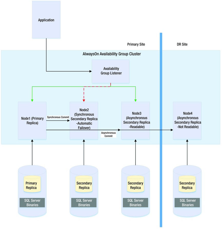
Figure 11-8. AlwaysOn Availability Group topology
![]() Note AlwaysOn Availability Groups are discussed in more detail in Chapter 13 and Chapter 16.
Note AlwaysOn Availability Groups are discussed in more detail in Chapter 13 and Chapter 16.
If a page becomes corrupt in a database configured as a replica in an AlwaysOn Availability Group topology, then SQL Server attempts to fix the corruption by obtaining a copy of the pages from one of the secondary replicas. This means that a logical corruption can be resolved without you needing to perform a restore or for you to run DBCC CHECKDB with a repair option. However, automatic page repair does not work for the following page types:
- File Header page
- Database Boot page
- Allocation pages
- GAM (Global Allocation Map)
- SGAM (Shared Global Allocation Map)
- PFS (Page Free Space)
If the primary replica fails to read a page because it is corrupt, it first logs the page in the MSDB.dbo.suspect_pages table. It then checks that at least one replica is in the SYNCHRONIZED state and that transactions are still being sent to the replica. If these conditions are met, then the primary sends a broadcast to all replicas, specifying the PageID and LSN (log sequence number) at the end of the flushed log. The page is then marked as restore pending, meaning that any attempts to access it will fail, with error code 829.
After receiving the broadcast, the secondary replicas wait, until they have redone transactions up to the LSN specified in the broadcast message. At this point, they try to access the page. If they cannot access it, they return an error. If they can access the page, they send the page back to the primary replica. The primary replica accepts the page from the first secondary to respond.
The primary replica will then replace the corrupt copy of the page with the version that it received from the secondary replica. When this process completes, it updates the page in the MSDB.dbo.suspect_pages table to reflect that it has been repaired by setting the event_type column to a value of 5 (Repaired).
If the secondary replica fails to read a page while redoing the log because it is corrupt, it places the secondary into the SUSPENDED state. It then logs the page in the MSDB.dbo.suspect_pages table and requests a copy of the page from the primary replica. The primary replica attempts to access the page. If it is inaccessible, then it returns an error and the secondary replica remains in the SUSPENDED state.
If it can access the page, then it sends it to the secondary replica that requested it. The secondary replica replaces the corrupt page with the version that it obtained from the primary replica. It then updates the MSDB.dbo.suspect_pages table with an event_id of 5. Finally, it attempts to resume the AOAG session.
![]() Note It is possible to manually resume the session, but if you do, the corrupt page is hit again during the synchronization. Make sure you repair or restore the page on the primary replica first.
Note It is possible to manually resume the session, but if you do, the corrupt page is hit again during the synchronization. Make sure you repair or restore the page on the primary replica first.
Log shipping is a technology that you can use to implement disaster recovery. It works by backing up the transaction log on the principle server, copying it to the secondary server, and then restoring it. It is most appropriate to use log shipping in DR scenarios in which you require a load delay, because this is not possible with AOAG. As an example of where a load delay may be useful, consider a scenario in which a user accidently deletes all of the data from a table. If there is a delay before the database on the DR server is updated, then it is possible to recover the data for this table, from the DR server, and then repopulate the production server. This means that you do not need to restore a backup to recover the data. Log shipping is not appropriate for high availability, since there is no automatic failover functionality. The diagram in Figure 11-9 illustrates a log shipping topology.

Figure 11-9. Log Shipping topology
Recovery Modes
In a log shipping topology, there is always exactly one principle server, which is the production server. It is possible to have multiple secondary servers, however, and these servers can be a mix of DR servers and servers used to offload reporting.
When you restore a transaction log, you can specify three recovery modes: Recovery, NoRecovery, and Standby. The Recovery mode brings the database online, which is not supported with Log Shipping. The NoRecovery mode keeps the database offline so that more backups can be restored. This is the normal configuration for log shipping and is the appropriate choice for DR scenarios.
The Standby option brings the database online, but in a read-only state so that you can restore further backups. This functionality works by maintaining a TUF (Transaction Undo File). The TUF file records any uncommitted transactions in the transaction log. This means that you can roll back these uncommitted transactions in the transaction log, which allows the database to be more accessible (although it is read-only). The next time a restore needs to be applied, you can reapply the uncommitted transaction in the TUF file to the log before the redo phase of the next log restore begins.
Figure 11-10 illustrates a log shipping topology that uses both a DR server and a reporting server.

Figure 11-10. Log shipping with DR and reporting servers
Remote Monitor Server
Optionally, you can configure a monitor server in your log shipping topology. This helps you centralize monitoring and alerting. When you implement a monitor server, the history and status of all backup, copy, and restore operations are stored on the monitor server. A monitor server also allows you to have a single alert job, which is configured to monitor the backup, copy, and restore operations on all servers, as opposed to it needing separate alerts on each server in the topology.
![]() Caution If you wish to use a monitor server, it is important to configure it when you set up log shipping. After log shipping has been configured, the only way to add a monitor server is to tear down and reconfigure log shipping.
Caution If you wish to use a monitor server, it is important to configure it when you set up log shipping. After log shipping has been configured, the only way to add a monitor server is to tear down and reconfigure log shipping.
Failover
Unlike other high availability and disaster recovery technologies, an amount of administrative effort is associated with failing over log shipping. To fail over log shipping, you must back up the tail-end of the transaction log, and copy it, along with any other uncopied backup files, to the secondary server.
You now need to apply the remaining transaction log backups to the secondary server in sequence, finishing with the tail-log backup. You apply the final restore using the WITH RECOVERY option to bring the database back online in a consistent state. If you are not planning to fail back, you can reconfigure log shipping with the secondary server as the new primary server.
![]() Note Log shipping is discussed in further detail in Chapter 14. Backups and restores are discussed in further detail in Chapter 15.
Note Log shipping is discussed in further detail in Chapter 14. Backups and restores are discussed in further detail in Chapter 15.
To meet your business objectives and non-functional requirements (NFRs), you need to combine multiple high availability and disaster recovery technologies together to create a reliable, scalable platform. A classic example of this is the requirement to combine an AlwaysOn Failover Cluster with AlwaysOn Availability Groups.
The reason you may need to combine these technologies is that when you use AlwaysOn Availability Groups in synchronous mode, which you must do for automatic failover, it can cause a performance impediment. As discussed earlier in this chapter, the performance issue is caused by the transaction being committed on the secondary server before being committed on the primary server. Clustering does not suffer from this issue, however, because it relies on a shared disk resource, and therefore the transaction is only committed once.
Therefore, it is common practice to first use a cluster to achieve high availability and then use AlwaysOn Availability Groups to perform DR and/or offload reporting. The diagram in Figure 11-11 illustrates a HA/DR topology that combines clustering and AOAG to achieve high availability and disaster recovery, respectively.

Figure 11-11. Clustering and AlwaysOn Availability Groups combined
The diagram in Figure 11-11 shows that the primary replica of the database is hosted on a two-node active/passive cluster. If the active node fails, the rules of clustering apply, and the shared storage, network name, and IP address are reattached to the passive node, which then becomes the active node. If both nodes are inaccessible, however, the availability group listener points the traffic to the third node of the cluster, which is situated in the DR site and is synchronized using log stream replication. Of course, when asynchronous mode is used, the database must be failed over manually by a DBA.
Another common scenario is the combination of a cluster and log shipping to achieve high availability and disaster recovery, respectively. This combination works in much the same way as clustering combined with AlwaysOn Availability Groups and is illustrated in Figure 11-12.

Figure 11-12. Clustering combined with log shipping
The diagram shows that a two-node active/passive cluster has been configured in the primary data center. The transaction log(s) of the database(s) hosted on this instance are then shipped to a stand-alone server in the DR data center. Because the cluster uses shared storage, you should also use shared storage for the backup volume and add the backup volume as a resource in the role. This means that when the instance fails over to the other node, the backup share also fails over, and log shipping continues to synchronize, uninterrupted.
![]() Caution If failover occurs while the log shipping backup or copy jobs are in progress, then log shipping may become unsynchronized and require manual intervention. This means that after a failover, you should check the health of your log shipping jobs.
Caution If failover occurs while the log shipping backup or copy jobs are in progress, then log shipping may become unsynchronized and require manual intervention. This means that after a failover, you should check the health of your log shipping jobs.
Summary
Understanding the concepts of availability is key to making the correct implementation choices for your applications that require high availability and disaster recovery. You should calculate the cost of downtime and compare this to the cost of implementing choices of HA/DR solutions to help the business understand the cost/benefit profile of each option. You should also be mindful of SLAs when choosing the technology implementation, since there could be financial penalties if SLAs are not met.
SQL Server provides a full suite of high availability and disaster recovery technologies, giving you the flexibility to implement a solution that best fits the needs of your data-tier applications. For high availability, you can implement either clustering or AlwaysOn Availability Groups (AOAG). Clustering uses a shared disk resource and failover occurs at the instance level. AOAG, on the other hand, synchronizes data at the database level by maintaining a redundant copy of the database with a synchronous log stream. Database mirroring is also available in SQL Server 2014, but it is a deprecated feature and will be removed in a future version of SQL Server.
To implement disaster recovery, you can choose to implement AOAG or log shipping. Log shipping works by backing up, copying, and restoring the transaction logs of the databases, whereas AOAG synchronizes the data using an asynchronous log stream.
It is also possible to combine multiple HA and DR technologies together in order to implement the most appropriate availability strategy. Common examples of this are combining clustering for high availability with AOAG or log shipping to provide DR.