
Chapter 18. Transfer Learning in JavaScript
In Chapter 17 you explored two methods for getting models into JavaScript: converting a Python-based model and using a preexisting model provided by the TensorFlow team. Aside from training from scratch, there’s one more option: transfer learning, where a model that was previously trained for one scenario has some of its layers reused for another. For example, a convolutional neural network for computer vision might have learned several layers of filters. If it was trained on a large dataset to recognize many classes, it may have very general filters that can be used for other scenarios.
To do transfer learning with TensorFlow.js, there are a number of options, depending on how the preexisting model is distributed. The possibilities fall into three main categories:
-
If the model has a model.json file, created by using the TensorFlow.js converter to convert it into a layers-based model, you can explore the layers, choose one of them, and have that become the input to a new model that you train.
-
If the model has been converted to a graph-based model, as are commonly found on TensorFlow Hub, you can connect feature vectors from it to another model to take advantage of its learned features.
-
If the model has been wrapped in a JavaScript file for easy distribution, this file will give you some handy shortcuts for prediction or transfer learning by accessing embeddings or other feature vectors.
In this chapter, you’ll explore all three. We’ll start by examining how you can access the prelearned layers in MobileNet, which you used as an image classifier in Chapter 17, and add them to your own model.
Transfer Learning from MobileNet
The MobileNet architecture defines a family of models trained primarily for on-device image recognition. They’re trained on the ImageNet dataset of over 10 million images, with 1,000 classes. With transfer learning, you can use their prelearned filters and change the bottom dense layers to match your classes instead of the 1,000 that the model was originally trained for.
To build an app that uses transfer learning, there are a number of steps that you’ll have to follow:
-
Download the MobileNet model and identify which layers to use.
-
Create your own model architecture with the outputs from MobileNet as its input.
-
Gather data into a dataset that can be used for training.
-
Train the model.
-
Run inference.
You’ll go through all of these here by building a browser application that captures images from the webcam of a hand making Rock/Paper/Scissors gestures, and then uses these to train a new model. The model will use the prelearned layers from MobileNet and add a new set of dense layers for your classes underneath.
Step 1. Download MobileNet and Identify the Layers to Use
The TensorFlow.js team hosts a number of preconverted models in Google Cloud Storage. You can find a list of URLs in the GitHub repo for this book, if you want to try them for yourself. There are several MobileNet models, including the one you’ll use in this chapter (mobilenet_v1_0.25_224/model.json).
To explore the model, create a new HTML file and call it mobilenet-transfer.html. In this file, you’ll load TensorFlow.js and an external file called index.js that you’ll create in a moment:
<html>
  <head>
    <script src="https://cdn.jsdelivr.net/npm/@tensorflow/tfjs@latest">
    </script>
  </head>
  <body></body>
  <script src="index.js"></script>
</html>
Next, create the index.js file that the preceding HTML is referring to. This will contain an asynchronous method that downloads the model and prints its summary:
async function init(){
  const url = 'https://storage.googleapis.com/tfjs-
models/tfjs/mobilenet_v1_0.25_224/model.json'

  const mobilenet = await tf.loadLayersModel(url);
  console.log(mobilenet.summary())
}

init()
If you look at the model.summary output in the console and scroll to the bottom, you’ll see something like Figure 18-1.
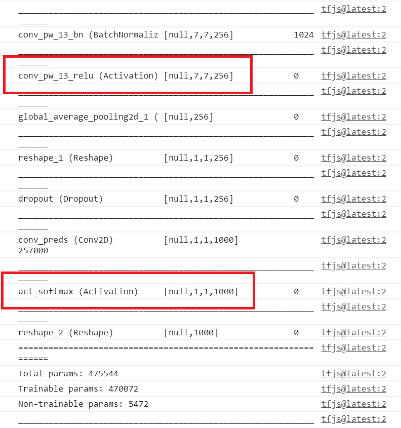
Figure 18-1. Output of model.summary for the MobileNet JSON model
The key to transfer learning with MobileNet is to look for the activation layers. As you can see, there are two right at the bottom. The last one has 1,000 outputs, which corresponds to the 1,000 classes that MobileNet supports. So, if you want the learned activation layers—in particular, the learned convolutional filters—look for activation layers above this, and note their names. As you can see in Figure 18-1, the last activation layer in the model, before the final one, is called conv_pw_13_relu. You can use that (or indeed, any activation layers before it) as your outputs from the model if you want to do transfer learning.
Step 2. Create Your Own Model Architecture with the Outputs from MobileNet as Its Input
When designing a model, you typically design all your layers, starting with the input layer and ending with the output one. With transfer learning, you will pass input to the model that you are transferring from, and you will create new output layers. Consider Figure 18-2—this is the rough, high-level architecture of MobileNet. It takes in images of dimension 224✕224✕3 and passes them through a neural network architecture, giving you an output of 1,000 values, each of which is the probability that the image contains the relevant class.

Figure 18-2. High-level MobileNet architecture
Earlier you looked at the innards of that architecture and identified the last activation convolutional layer, called conv_pw_13_relu. You can see what the architecture looks like with this layer included in Figure 18-3.
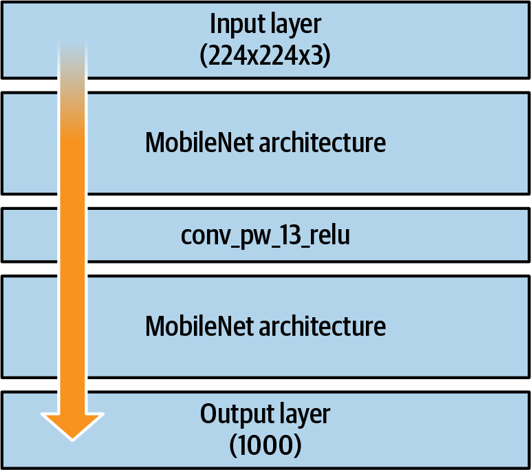
Figure 18-3. High-level MobileNet architecture showing conv_pw_13_relu
The MobileNet architecture still has 1,000 classes that it recognizes, none of which are the ones you want to implement (a hand making gestures for the game Rock Paper Scissors). You’ll need a new model that is trained on these three classes. You could train it from scratch and learn all the filters that will give you the features to distinguish them, as seen in earlier chapters, or you can take the prelearned filters from MobileNet, using the architecture all the way up to conv_pw_13_relu, and feed that to a new model that classifies only three classes. See Figure 18-4 for an abstraction of this.
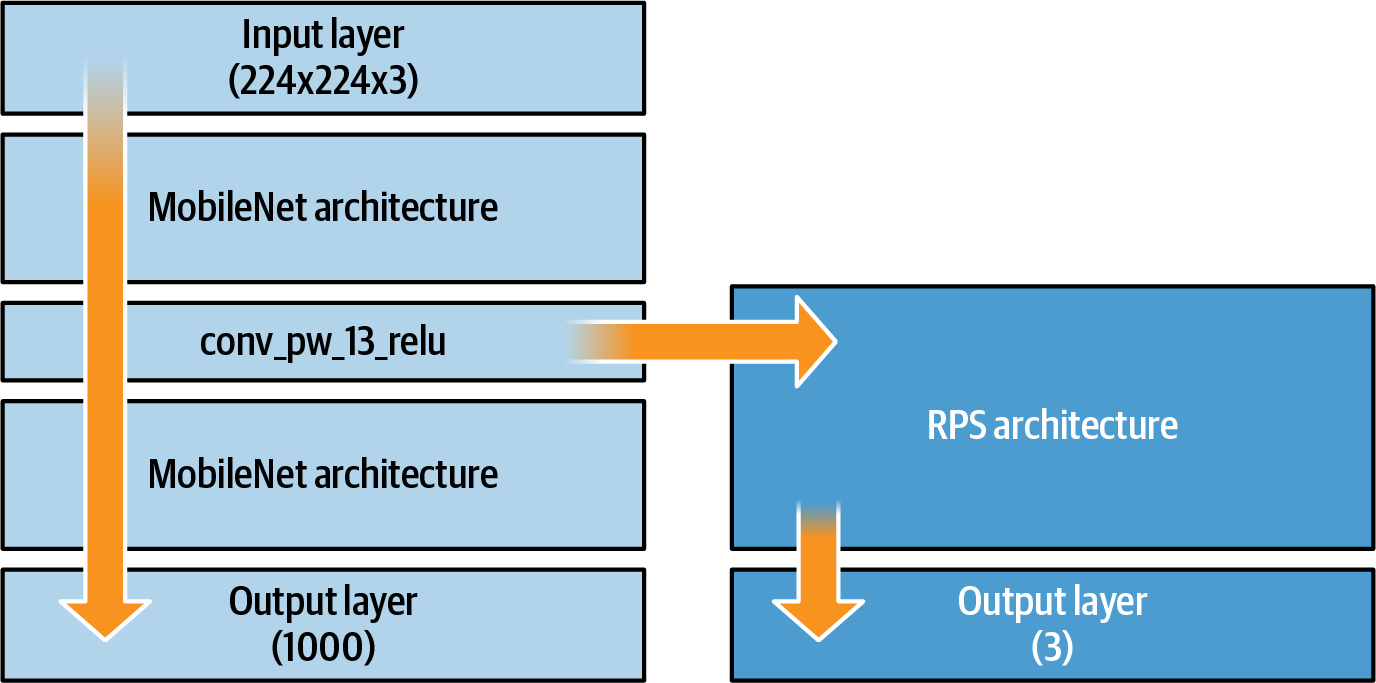
Figure 18-4. Transfer learning from conv_pw_13_relu to a new architecture
To implement this in code, you can update your index.js to the following:
let mobilenet

async function loadMobilenet() {
  const mobilenet = await tf.loadLayersModel(url);
  const layer = mobilenet.getLayer('conv_pw_13_relu');
  return tf.model({inputs: mobilenet.inputs, outputs: layer.output});
}

async function init(){
  mobilenet = await loadMobilenet()
  model = tf.sequential({
  layers: [
    tf.layers.flatten({inputShape: mobilenet.outputs[0].shape.slice(1)}),
    tf.layers.dense({ units: 100, activation: 'relu'}),
    tf.layers.dense({ units: 3, activation: 'softmax'})
  ]
  });
  console.log(model.summary())
}

init()
The loading of mobilenet has been put into its own async function. Once the model has finished loading, the conv_pw_13_relu layer can be extracted from it using the getLayer method. The function will then return a model with its inputs set to mobilenet’s inputs and its outputs set to conv_pw_13_relu’s outputs. This is visualized by the right-pointing arrow in Figure 18-4.
Once this function returns, you can create a new sequential model. Note the first layer in it—it’s a flatten of the mobilenet outputs (i.e., the conv_pw_13_relu outputs), which then feeds into a dense layer of 100 neurons, which feeds into a dense layer of 3 neurons (1 each for Rock, Paper, and Scissors).
If you now do a model.fit on this model, you’ll train it to recognize three classes—but instead of learning all the filters to identify features in the image from scratch, you’ll be able to use the ones that were previously learned by MobileNet. Before you can do that, though, you’ll need some data. You’ll see how to gather that in the next step.
Step 3. Gather and Format the Data
For this example, you’ll use the webcam in the browser to capture images of a hand making Rock/Paper/Scissors gestures. Capturing data from the webcam is beyond the scope of this book, so I won’t go into detail on it here, but there’s a webcam.js file in the GitHub repo for this book (created by the TensorFlow team) that can handle everything for you. This captures images from the webcam and returns them in a TensorFlow-friendly format as batched images. It also handles all the tidying-up code from TensorFlow.js that the browser will need to avoid memory leaks. Here’s a snippet from the file:
capture() {
  return tf.tidy(() => {
    // Read the image as a tensor from the webcam <video> element.
    const webcamImage = tf.browser.fromPixels(this.webcamElement);
    const reversedImage = webcamImage.reverse(1);
    // Crop the image so we're using the center square of the rectangle.
    const croppedImage = this.cropImage(reversedImage);
    // Expand the outermost dimension so we have a batch size of 1.
    const batchedImage = croppedImage.expandDims(0);
    // Normalize the image between -1 and 1. The image comes in between
    // 0-255, so we divide by 127 and subtract 1.
    return batchedImage.toFloat().div(tf.scalar(127)).sub(tf.scalar(1));
  });
}
You can include this .js file in your HTML with a simple <script> tag:
<script src="webcam.js"></script>
You can then update the HTML with a <div> to hold the video preview from the webcam, buttons that the user will select to capture samples of Rock/Paper/Scissors gestures, and <div>s to output the number of samples captured. Here’s what it should look like:
<html>
  <head>
    <script src="https://cdn.jsdelivr.net/npm/@tensorflow/tfjs@latest">
    </script>
    <script src="webcam.js"></script>
  </head>
  <body>
    <div>
      <video autoplay playsinline muted id="wc" width="224" height="224"/>
    </div>
    <button type="button" id="0" onclick="handleButton(this)">Rock</button>
    <button type="button" id="1" onclick="handleButton(this)">Paper</button>
    <button type="button" id="2" onclick="handleButton(this)">Scissors</button>
      <div id="rocksamples">Rock Samples:</div>
      <div id="papersamples">Paper Samples:</div>
      <div id="scissorssamples">Scissors Samples:</div>
  </body>
  <script src="index.js"></script>
</html>
Then all you need to do is add a const to the top of your index.js file that initializes the webcam with the ID of the <video> tag in your HTML:
const webcam = new Webcam(document.getElementById('wc'));
You can then initialize the webcam within your init function:
await webcam.setup();
Running the page will now give you a webcam preview along with the three buttons (see Figure 18-5).

Figure 18-5. Getting the webcam preview to work
Note that if you don’t see the preview, you should see an icon like the one highlighted at the top of this figure in the Chrome status bar. If it has a red line through it, you need to give the browser permission to use the webcam, after which you should see the preview. The next thing you need to do is capture the images and put them in a format that makes it easy for you to train the model you created in step 2.
As TensorFlow.js cannot take advantage of built in datasets like Python, you’ll have to roll your own dataset class. Fortunately, it’s not as difficult as it sounds. In JavaScript, create a new file called rps-dataset.js. Construct it with an array for the labels, as follows:
class RPSDataset {
  constructor() {
    this.labels = []
  }
}
Every time you capture a new example of a Rock/Paper/Scissors gesture from the webcam, you’ll want to add it to the dataset. This can be achieved with an addExample method. The examples will be added as xs. Note that this will not add the raw image, but the classification of the image by the truncated mobilenet. You’ll see this in a moment.
The first time you call this, the xs will be null, so you’ll create the xs using the tf.keep method. This, as its name suggests, prevents a tensor from being destroyed in a tf.tidy call. It also pushes the label to the labels array created in the constructor. For subsequent calls, the xs will not be null, so you’ll copy the xs into an oldX and then concat the example to that, making that the new xs. You’ll then push the label to the labels array and dispose of the old xs:
addExample(example, label) {
  if (this.xs == null) {
    this.xs = tf.keep(example);
    this.labels.push(label);
  } else {
    const oldX = this.xs;
    this.xs = tf.keep(oldX.concat(example, 0));
    this.labels.push(label);
    oldX.dispose();
  }
}
Following this approach, your labels will be an array of values. But to train the model you need them as a one-hot encoded array, so you’ll need to add a helper function to your dataset class. This JavaScript will encode the labels array into a number of classes specified by the numClasses parameter:
encodeLabels(numClasses) {
  for (var i = 0; i < this.labels.length; i++) {
    if (this.ys == null) {
      this.ys = tf.keep(tf.tidy(
          () => {return tf.oneHot(
              tf.tensor1d([this.labels[i]]).toInt(), numClasses)}));
    } else {
      const y = tf.tidy(
          () => {return tf.oneHot(
              tf.tensor1d([this.labels[i]]).toInt(), numClasses)});
      const oldY = this.ys;
      this.ys = tf.keep(oldY.concat(y, 0));
      oldY.dispose();
      y.dispose();
    }
  }
}
The key is the tf.oneHot method, which, as its name suggests, encodes its given parameters into a one-hot encoding.
In your HTML you added the three buttons and specified their onclick to call a function called handleButton, like this:
<button type="button" id="0" onclick="handleButton(this)">Rock</button>
<button type="button" id="1" onclick="handleButton(this)">Paper</button>
<button type="button" id="2" onclick="handleButton(this)">Scissors</button>
You can implement this in your index.js script by switching on the element ID (which is 0, 1, or 2 for Rock, Paper, and Scissors, respectively), turning that into a label, capturing the webcam image, calling the predict method on mobilenet, and adding the result as an example to the dataset using the method you created earlier:
function handleButton(elem){
  label = parseInt(elem.id);
  const img = webcam.capture();
  dataset.addExample(mobilenet.predict(img), label);
}
It’s worth making sure you understand the addExample method before going further. While you could create a dataset that captures the raw images and adds them to a dataset, recall Figure 18-4. You created the mobilenet object with the output of conv_pw_13_relu. By calling predict, you’ll get the output of that layer. And if you look back to Figure 18-1, you’ll see that the output was [?, 7, 7, 256]. This is summarized in Figure 18-6.
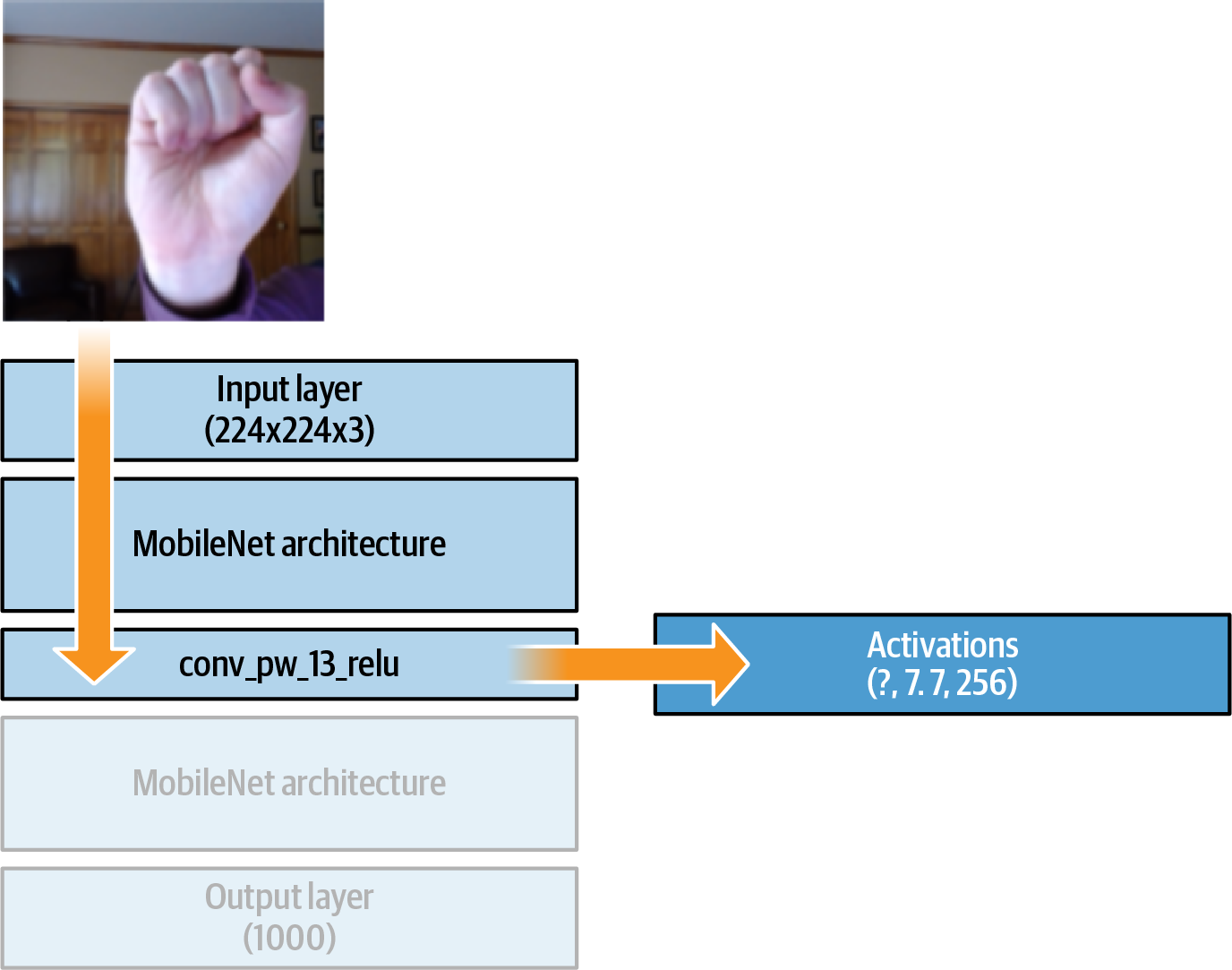
Figure 18-6. Results of mobilenet.predict
Recall that with a CNN, as the image progresses through the network a number of filters are learned, and the results of these filters are multiplied into the image. They usually get pooled and passed to the next layer. With this architecture, by the time the image reaches the output layer, instead of a single color image you’ll have 256 7×7 images, which are the results of all the filter applications. These can then be fed into a dense network for classification.
You can also add code to this to update the user interface, counting the number of samples added. I’ve omitted it here for brevity, but it’s all in the GitHub repo.
Don’t forget to add the rps-dataset.js file to your HTML using a <script> tag:
<script src="rps-dataset.js"></script>
In the Chrome developer tools you can add breakpoints and watch variables. Run your code, and add a watch to the dataset variable and a breakpoint to the dataset.addExample method. Click one of the Rock/Paper/Scissors buttons and you’ll see the dataset get updated. In Figure 18-7 you can see the results after I clicked each of the three buttons.
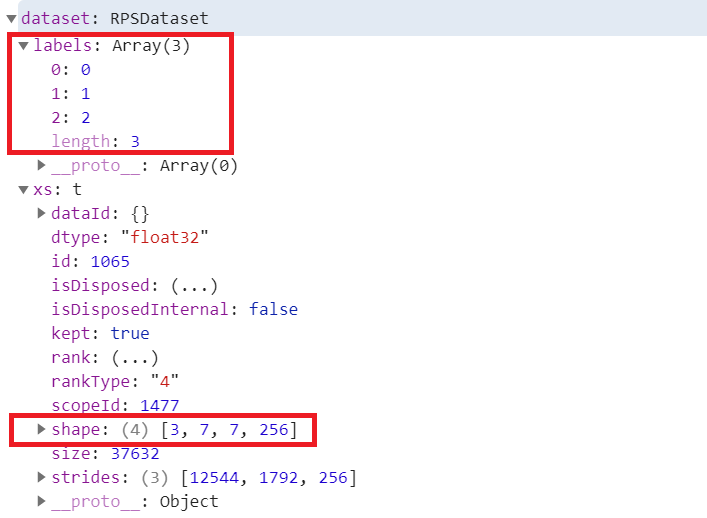
Figure 18-7. Exploring the dataset
Note that the labels array is set up with 0, 1, 2 for the three labels. It hasn’t been one-hot encoded yet. Also, within the dataset you can see a 4D tensor with all of the gathered data. The first dimension (3) is the number of samples gathered. The subsequent dimensions (7, 7, 256) are the activations from mobilenet.
You now have a dataset that can be used to train your model. At runtime you can have your users click each of the buttons to gather a number of samples of each type, which will then be fed into the dense layers that you specified for classification.
Step 4. Train the Model
This app will work by having a button to train the model. Once the training is complete, you can then press a button to start the model predicting what it sees in the webcam, and another to stop predicting.
Add the following HTML to your page to add these three buttons, and some <div> tags to hold the output. Note that the buttons call methods called doTraining, startPredicting, and stopPredicting:
<button type="button" id="train" onclick="doTraining()">
  Train Network
</button>
<div id="dummy">
  Once training is complete, click 'Start Predicting' to see predictions
  and 'Stop Predicting' to end
</div>
<button type="button" id="startPredicting" onclick="startPredicting()">
  Start Predicting
</button>
<button type="button" id="stopPredicting" onclick="stopPredicting()">
  Stop Predicting
</button>
<div id="prediction"></div>
WIthin your index.js, you can then add a doTraining method and populate it:
function doTraining(){
  train();
}
WIthin the train method you can then define your model architecture, one-hot encode the labels, and train the model. Note the first layer in the model has its inputShape defined as the output shape of mobilenet, and you previously specified the mobilenet object’s output to be the conv_pw_13_relu:
async function train() {
  dataset.ys = null;
  dataset.encodeLabels(3);
  model = tf.sequential({
    layers: [
      tf.layers.flatten({inputShape: mobilenet.outputs[0].shape.slice(1)}),
      tf.layers.dense({ units: 100, activation: 'relu'}),
      tf.layers.dense({ units: 3, activation: 'softmax'})
    ]
  });
  const optimizer = tf.train.adam(0.0001);
  model.compile({optimizer: optimizer, loss: 'categoricalCrossentropy'});
  let loss = 0;
  model.fit(dataset.xs, dataset.ys, {
    epochs: 10,
    callbacks: {
      onBatchEnd: async (batch, logs) => {
        loss = logs.loss.toFixed(5);
        console.log('LOSS: ' + loss);
      }
    }
  });
}
This will train the model for 10 epochs. You can adjust this as you see fit depending on the loss in the model.
Earlier you defined the model in init.js, but it’s a good idea to move it here instead and keep the init function just for initialization. So, your init should look like this:
async function init(){
  await webcam.setup();
  mobilenet = await loadMobilenet()
}
At this point you can practice making Rock/Paper/Scissors gestures in front of the webcam. Press the appropriate button to capture an example of a given class. Repeat this about 50 times for each of the classes, and then press Train Network. After a few moments, the training will complete, and in the console you’ll see the loss values. In my case the loss started at about 2.5 and ended at .0004, indicating that the model was learning well.
Note that 50 samples is more than enough for each class, because when we add the examples to the dataset, we add the activated examples. Each image gives us 256 7✕7 images to feed into the dense layers, so 150 samples gives us 38,400 overall items for training.
Now that you have a trained model, you can try doing predictions with it!
Step 5. Run Inference with the Model
Having completed step 4, you should have code that gives you a fully trained model. You also created HTML buttons to start and stop predicting. These were configured to call the startPredicting and stopPredicting methods, so you should create them now. Each one should just set an isPredicting Boolean to true/false, respectively, for whether you want to predict or not. After that they call the predict method:
function startPredicting(){
  isPredicting = true;
  predict();
}

function stopPredicting(){
  isPredicting = false;
  predict();
}
The predict method then can use your trained model. It will capture the webcam input and get the activations by calling mobilenet.predict with the image. Then, once it has the activations, it can pass them to the model to get a prediction. As the labels were one-hot encoded, you can call argMax on the predictions to get the likely output:
async function predict() {
  while (isPredicting) {
    const predictedClass = tf.tidy(() => {
      const img = webcam.capture();
      const activation = mobilenet.predict(img);
      const predictions = model.predict(activation);
      return predictions.as1D().argMax();
    });
    const classId = (await predictedClass.data())[0];
    var predictionText = "";
    switch(classId){
      case 0:
        predictionText = "I see Rock";
        break;
      case 1:
        predictionText = "I see Paper";
        break;
      case 2:
        predictionText = "I see Scissors";
        break;
    }
    document.getElementById("prediction").innerText = predictionText;


    predictedClass.dispose();
    await tf.nextFrame();
  }
}
With 0, 1, or 2 as the result, you can then write the value to the prediction <div> and clean up.
Note that this is gated on the isPredicting Boolean, so you can turn predictions on or off with the relevant buttons. Now when you run the page you can collect samples, train the model, and run inference. See Figure 18-8 for an example, where it classified my hand gesture as Scissors!

Figure 18-8. Running inference in the browser with the trained model
From this example, you saw how to build your own model for transfer learning. Next you’ll explore an alternative approach using graph-based models stored in TensorFlow Hub.
Transfer Learning from TensorFlow Hub
TensorFlow Hub is an online library of reusable TensorFlow models. Many of the models have already been converted into JavaScript for you—but when it comes to transfer learning, you should look for “image feature vector” model types, and not the full models themselves. These are models that have already been pruned to output the learned features. The approach here is a little different from the example in the previous section, where you had activations output from MobileNet that you could then transfer to your custom model. Instead, a feature vector is a 1D tensor that represents the entire image.
To find a MobileNet model to experiment with, visit TFHub.dev, choose TF.js as the model format you want, and select the MobileNet architecture. You’ll see lots of options of models that are available to you, as shown in Figure 18-9.
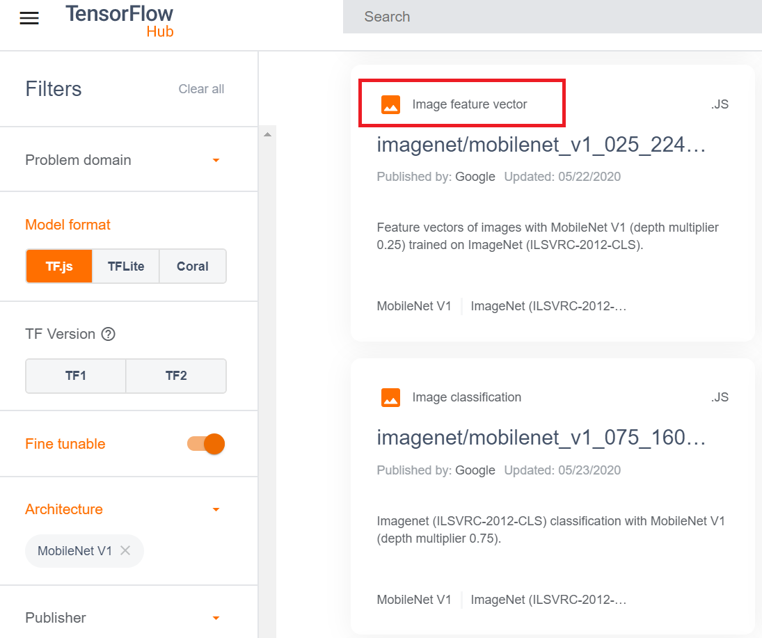
Figure 18-9. Using TFHub.dev to find JavaScript models
Find an image feature vector model (I’m using 025_224), and select it. In the “Example use” section on the model’s details page you’ll find code indicating how to download the image—for example:
tf.loadGraphModel("https://tfhub.dev/google/tfjs-model/imagenet/
    mobilenet_v1_025_224/feature_vector/3/default/1", { fromTFHub: true })
You can use this to download the model so you can inspect the dimensions of the feature vector. Here’s a simple HTML file with this code in it that classifies an image called dog.jpg, which should be in the same directory:
<html>
<head>
<script src="https://cdn.jsdelivr.net/npm/@tensorflow/tfjs@latest"> </script>
</head>
<body>
  <img id="img" src="dog.jpg"/>
</body>
</html>
<script>
async function run(){
  const img = document.getElementById('img');
  model = await tf.loadGraphModel('https://tfhub.dev/google/tfjs-model/imagenet/
      mobilenet_v1_025_224/feature_vector/3/default/1', {fromTFHub: true});
  var raw = tf.browser.fromPixels(img).toFloat();
  var resized = tf.image.resizeBilinear(raw, [224, 224]);
  var tensor = resized.expandDims(0);
  var result = await model.predict(tensor).data();
  console.log(result)
}

run();

</script>
When you run this and look in the console, you’ll see the output from this classifier (Figure 18-10). If you are using the same model as me, you should see a Float32Array with 256 elements in it. Other MobileNet versions may have output of different sizes.
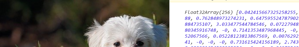
Figure 18-10. Exploring the console output
Once you know the output shape of the image feature vector model, you can use it for transfer learning. So, for example, for the Rock Paper Scissors example you could use an architecture like that in Figure 18-11.
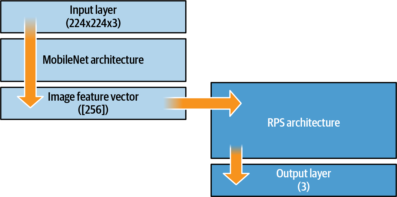
Figure 18-11. Transfer learning using image feature vectors
Now you can edit the code for your transfer learning Rock Paper Scissors app by changing how and where you load the model from, and by amending the classifier to accept the image feature vector instead of the activated features, as earlier.
If you want to load your model from TensorFlow Hub, you just update the loadMobilenet function like this:
async function loadMobilenet() {
  const mobilenet =
    await tf.loadGraphModel("https://tfhub.dev/google/tfjs-model/imagenet/
    mobilenet_v1_050_160/feature_vector/3/default/1", {fromTFHub: true})
  return mobilenet
}
And then, in your train method, where you define the model for the classification, you update it to receive the output from the image feature vector ([256]) to the first layer. Here’s the code:
model = tf.sequential({
  layers: [
    tf.layers.dense({ inputShape: [256], units: 100, activation: 'relu'}),
    tf.layers.dense({ units: 3, activation: 'softmax'})
  ]
});
Note that this shape will be different for different models. You can use code like the HTML shown earlier to find it if it isn’t published for you.
Once this is done, you can do transfer learning from the model in TensorFlow Hub using JavaScript!
Using Models from TensorFlow.org
Another source for models for JavaScript developers is TensorFlow.org (see Figure 18-12). The models provided here, for image classification, object detection, and more, are ready for immediate use. Clicking on any of the links will take you to a GitHub repository of JavaScript classes which wrap the graph-based models with logic to make using them much easier.

Figure 18-12. Browsing models on TensorFlow.org
In the case of MobileNet, you can use the model with a <script> include like this:
<script src="https://cdn.jsdelivr.net/npm/@tensorflow-models/[email protected]">
</script>
If you take a look at the code you’ll notice two things. First, the set of labels is encoded within the JavaScript, giving you a handy way of seeing the inference results without a secondary lookup. You can see a snippet of the code here:
var i={
 0:"tench, Tinca tinca",
 1:"goldfish, Carassius auratus",
 2:"great white shark, white shark, man-eater, man-eating shark, Carcharodon
 carcharias",
 3:"tiger shark, Galeocerdo cuvieri"
...
Additionally, toward the bottom of this file you’ll see a number of models, layers, and activations from TensorFlow Hub that you can load into JavaScript variables. For example, for version 1 of MobileNet you may see an entry like this:
n={"1.00":
{.25:"https://tfhub.dev/google/imagenet/mobilenet_v1_025_224/classification/1",
 "0.50":"https://tfhub.dev/google/imagenet/mobilenet_v1_050_224/classification/1",
.75:"https://tfhub.dev/google/imagenet/mobilenet_v1_075_224/classification/1",
"1.00":"https://tfhub.dev/google/imagenet/mobilenet_v1_100_224/classification/1"
}
The values .25, .50, .75, etc. are “width multiplier” values. These are used to construct smaller, less computationally expensive models; you can find details in the original paper introducing the architecture.
The code offers many handy shortcuts. For example, when running inference on an image, compare the following listing to the one shown a little earlier, where you used MobileNet to get an inference for the dog image. Here’s the full HTML:
<html>
<head>
<script src="https://cdn.jsdelivr.net/npm/@tensorflow/tfjs@latest">
</script>
<script src="https://cdn.jsdelivr.net/npm/@tensorflow-models/[email protected]"> </script>
</head>
<body>
  <img id="img" src="dog.jpg"/>
</body>
</html>
<script>
async function run(){
  const img = document.getElementById('img');
  mobilenet.load().then(model => {
    model.classify(img).then(predictions => {
      console.log('Predictions: ');
      console.log(predictions);
    });

  });
}

run();

</script>
Note how you don’t have to preconvert the image into tensors in order to do the classification. This code is much cleaner, and allows you to just focus on your predictions. To get embeddings, you can use model.infer instead of model.classify like this:
embeddings = model.infer(img, embedding=true);
console.log(embeddings);
So, if you wish, you could create a transfer learning scenario from MobileNet using these embeddings.
Summary
In this chapter you took a look at a variety of options for transfer learning from preexisting JavaScript-based models. As there’s a range of different model implementation types, there are also a number of options for accessing them for transfer learning. First, you saw how to use the JSON files created by the TensorFlow.js converter to explore the layers of the model and choose one to transfer from. The second option is to use graph-based models. This is the favored type of model on TensorFlow Hub (because they generally give faster inference), but you lose a little of the flexibility of being able to choose the layer to do the transfer learning from. When using this method, the JavaScript bundle that you download doesn’t contain the full model, but instead truncates it as the feature vector output. You transfer from this to your own model. Finally, you saw how to work with the prewrapped JavaScript models made available by the TensorFlow team on TensorFlow.org, which include helper functions for accessing the data, inspecting the classes, as well as getting the embeddings or other feature vectors from the model so they can be used for transfer learning.
In general, I would recommend taking the TensorFlow Hub approach and using models with prebuilt feature vector outputs when they’re available—but if they aren’t, it’s good to know that TensorFlow.js has a flexible enough ecosystem to allow for transfer learning in a variety of ways!