Chapter 6
Controlling Formulas

Although you can go a long way with simple formulas, it is also possible to build extremely powerful formulas. The topics in this chapter explain the finer points of formula operators, date math, and how Excel distinguishes between cutting and copying cells referenced in formulas.

Formula Operators

Excel offers the mathematical operators shown in Table 6.1.

Order of Operations

When a formula contains many calculations, Excel evaluates the formula in a certain order. Rather than calculating from left to right as a calculator might, Excel performs certain types of calculations, such as multiplication, before calculations such as addition.

You can override the default order of operations with parentheses. If you do not use parentheses, Excel uses the following order of operations:

1. Unary minus is evaluated first.

2. Exponents are evaluated next.

3. Multiplication and division are handled next, in a left-to-right manner.

4. Addition and subtraction are handled next, in a left-to-right manner.

The following sections provide some examples of order of operations.

Unary Minus Example

The unary minus is always evaluated first. Think about when you use exponents to raise a number to a power. If you raise –2 to the second power, Excel calculates (–2) × (–2), which is +4. Therefore, the formula =–2^2 evaluates to 4.

If you raise –2 to the third power, Excel calculates (–2) × (–2) × (–2). Multiplying –2 by –2 results in +4, and multiplying +4 by –2 results in –8. Therefore, the simple formula =–2^3 generates –8.

You need to understand a subtle but important distinction. When Excel encounters the formula =–2^3, it evaluates the unary minus first. If you want the exponent to happen first and then have the unary minus applied, you have to write the formula as =–(2^3). However, in a formula such as =100–2^3, the minus sign is considered to be a subtraction operator and not a unary minus sign. In this case, 2^3 is evaluated as 8, and then 8 is subtracted from 100. To indicate a unary minus, use =100–(–2^3).

Addition and Multiplication Example

The order of operations is important when you are mixing addition/subtraction with multiplication/division. For example, if you want to add 20 to 30 and then multiply by 1.06 to calculate a total with tax, the following formula leads to the wrong result:

=20+30*1.06

The result you are looking for is 53. However, the Evaluate Formula dialog box shows that Excel calculates the formula =20+30*1.06 like so (see Figure 6.1):

1.06 × 30 = 31.8
31.8 + 20 = 51.8

Excel’s answer is $1.20 less than expected because the formula is not written with the default order of operations in mind.

To force Excel to do the addition first, you need to enclose the addition in parentheses:

=(20+30)*1.06

The addition in parentheses is done first, and then 50 is multiplied by 1.06 to get the correct answer of $53.

Stacking Multiple Parentheses

If you need to use multiple sets of parentheses when doing math by hand, you might write math formulas with square brackets and curly braces, like this:

{3-[6*4*3-(3-6)+2]/27}*14

In Excel, you use multiple sets of parentheses, as follows:

=(3-(6*4*3-(3-6)+2)/27)*14

Formulas with multiple parentheses in Excel are confusing. Excel does two things to try to improve this situation:

• As you type a formula, Excel colors the parentheses in a set order: black, red, purple, green, violet, topaz, aquamarine, blue. The colors then repeat starting with red. By far, the most common problem is having one too few or one too many parentheses. By using red as the second color, the last parenthesis in most unbalanced equations is red. Excel uses black only for the first parenthesis and for the closing match to that parenthesis. This means if your last parenthesis in the formula is not black, you have the wrong number of parentheses.

• When you type a closing parenthesis, Excel shows the opening parenthesis in bold for a fraction of a second. This would be more helpful if Excel kept the opening parenthesis in bold for 5 seconds or 20 seconds.

Understanding Error Messages in Formulas

Don’t be frustrated when a formula returns an error result. This eventually happens to everyone. The key is to understand the difference between the various error values so that you can begin to troubleshoot the problem.

As you enter formulas, you might encounter some errors, including those listed next:

• #VALUE!—This error indicates that you are trying to do math with nonnumeric data. For example, the formula =4+"apple" returns a #VALUE! error. This error also occurs if you try to enter an array formula but fail to use Ctrl+Shift+Enter, as described in Chapter 12, “Array Formulas and Names in Excel.”

• #DIV/0!—This error occurs when a number is divided by zero—that is, when a fraction’s denominator evaluates to zero.

• #REF!—This error occurs when a cell reference is not valid. For example, this error can occur if one of the cells referenced in the formula has been deleted. It can also occur if you cut and paste another cell over a cell referenced in this formula. You may also get this error if you are using Dynamic Data Exchange (DDE) formulas to link to external systems and those systems are not running.

• #N/A!—This error occurs when a value is not available to a function or a formula. #N/A! errors most often occur because of key values not being found during lookup functions. They can occur as a result of HLOOKUP, LOOKUP, MATCH, or VLOOKUP. They can also result when an array formula has one argument that is not the same shape as the other arguments or when a function omits one or more required arguments. Interestingly, when an #N/A! error enters a range, all subsequent calculations that refer to the range have a value of #N/A!.

• NULL!—This error usually indicates that two cell references by a formula are separated by a space instead of a colon or comma. The space operator is the intersection operator. If there are no cells in common between the two references, a NULL! error appears.

• SPILL!—This error is new in Office 365 after the summer of 2018. If you use one of the new =A1:A100 formulas in cell C1 and some non-blank cells appear in the 100 cells needed for the response, you will see a SPILL! error in all cells. Other causes of the SPILL error include the formula spilling beyond the edge of the worksheet or running out of memory.

• #FIELD!—This error is new in 2018 and indicates a problem with a Linked Data Type. The error occurs if the referenced field is not available in a linked data type or if the formula is referencing a cell that does not contain a linked data type. Here is an example: Type Florida in cell A1 and use the Data Types gallery on the Data tab to mark that cell as geography. You can use =A1.Population to retrieve the population. However, if you change cell A1 to Apple, the #FIELD! error will appear because Excel does not have a geography definition for Apple.

• #CALC—New as of late 2018 or early 2019 for Office 365 customers. The calculation engine can’t resolve the formula yet, but the syntax might be supported in the future. The Excel team has plans for a series of new functions that will roll out over several releases, and the #CALC error is needed if they plan on rolling out part of a two-function solution.

• ######—This is not really an error. Instead, it means that the result is too wide to display in the current column width, so you need to make the column wider to see the actual result. Although ###### usually means the column is not wide enough, it can also appear if you are subtracting one date or time from another and end up with a negative amount. Excel does not allow negative dates or times unless you switch to the 1904 Date System.

In Figure 6.2, cell E17 is a simple SUM function. It is returning an #N/A error because cell E11 contains the same error. Cell E11 contains the formula =D11*C11. The root cause of the problem is the VLOOKUP function in cell D11. Because Fig cannot be found in the product table in $G$7:$H$9, the VLOOKUP function returns #N/A.

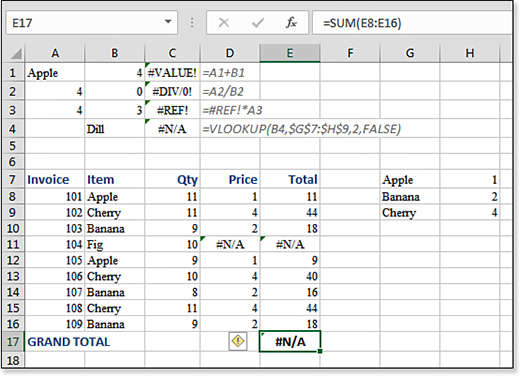
Figure 6.2 shows only a small table, so it is relatively easy to find the earlier #N/A errors. However, when you’re totaling 100,000 rows, it can be difficult to find the one offending cell. To track down errors, follow these steps:

1. Select the cell that shows the final error. To the left of that cell, you should see an exclamation point in a yellow diamond.

2. Hover the cursor over the yellow diamond to reveal a drop-down menu arrow.

3. From the drop-down menu, select Trace Error. Excel draws in red arrows pointing back to the source of the error, as shown in Figure 6.3. For example, from the original #N/A! error in cell D11, blue arrows demonstrate what cells were causing the error. To remove the arrows, use the Remove Arrows command on the Formulas tab.

   

Using Formulas to Join Text

You use the ampersand (&) operator when you need to join text. In Excel, the & operator is known as the concatenation operator.

When using the & operator, you often need to include a space between the two items that are combined to improve the appearance of the output. For example, if the cells contain first name and last name, you want to have a space between the names. To include a space between cells, you follow the & with a space enclosed in quotes, as in &" ". As shown in Figure 6.4, the formula =A2&" "&B2 joins the first name and last name with a space in between.

Joining Text and a Number

In many cases, you can use the & operator to join text with a number or a date. In Figure 6.5, the formula in cell E2 joins the words “The price is $” with the result of the calculation in cell D2. Although D2 is formatted to show only two decimal places, the underlying answer has more decimal places. The regular concatenation formula in E2 shows the extra decimal places. To fix the problem, use the TEXT() function around D2 in the formula. Specify any valid numeric formatting code in quotes as the second argument. The corrected formula in E6 uses TEXT(D6,"#,##0.00").

When you join text to a date or time, you see the serial number that Excel stores behind the scenes instead of the date. Cell E3 in Figure 6.5 shows the result of joining text with a date. Use the TEXT() function around the date to format it as shown in cell E7.

Copying Versus Cutting a Formula

In Figure 6.6, the formula in cell C4 references A4+B4. Because there are no dollar signs within the formula, those are relative references.

If you copy cell C4 and paste it to cell G2, the formula works perfectly, adding the two numbers to the left of G2. However, if you cut C4 and paste to F6, the formula continues to point to cells A4+B4, as shown in Figure 6.7. Whereas cutting and copying are relatively similar in applications such as Word, they are very different in Excel. It is important to understand the effect of cutting a formula in Excel in contrast to copying the formula. When you cut a formula, the formula continues to point to the original precedents, no matter where you paste it.

A similar rule applies to the references mentioned in a formula. For example, in Figure 6.6, the formula in cell C4 points to A4 and B4. As long as you copy cell A4, you can paste it anywhere without changing the formula in C4. But if you would cut A4 and paste it elsewhere, the formula in C4 would update to reflect the new location.

Automatically Formatting Formula Cells

The rules for formatting the result of a formula seem to be inconsistent. Suppose that you have $1.23 in cell A1. All cells in the worksheet have the general format except cell A1.

If you enter =A1+3 in another cell with general format, the result automatically inherits the currency format of cell A1.

When you are referring to multiple cells in a formula, the resulting automatic format does not appear to follow a pattern. When you start the formula with an equal sign, either the format is copied from the first or the last cell referenced. When you use a plus sign, the format sometimes comes from the second, first, or last reference, and sometimes the format is a mix of two references.

If your formula is going to refer to multiple cells with different formatting, start the formula with an equal sign. Refer to the cell with the desired cell format first, but accept that you might have to explicitly format the resulting cell.

Using Date Math

Dates in Excel are stored as the number of days since January 1, 1900. For example, Excel stores the date Feb-17-2021 as 44244. In Figure 6.8, cell E1 contains the date. Cell E2 contains the formula =E1 and has been formatted to show a number.

This convenient system enables you to do some pretty simple math. For example, Figure 6.9 shows a range of invoice dates in column B. The payment terms for the invoice are in column D. You can calculate the due date by adding cells B2 and D2. Here is what actually happens in Excel’s calculation engine:

1. The date in cell B2—2/1/2018—is stored as 43132.

2. Excel adds 10 to that number to get the answer 43142.

3. Excel formats this number as a date, to yield 2/11/2018.

   

However, a frustrating problem can occur if the cell containing the formula has the wrong numeric format. For example, in Figure 6.10, the WORKDAY function in column D did not automatically convert the result to a date. It is important to recognize that dates in 2019–2021 fall in the range of 43,466 to 44,561. So, if you are expecting a date answer as the result of a formula and get a number in this range, the answer probably needs to have a date format applied.

To apply a date format, on the Home tab use the Number drop-down menu to choose the Date format. The answer in column D now appears correctly.

In general, most formulas that refer to a date cell are automatically formatted as a date. Most formulas that contain functions from the Date category are formatted as a date. (The WORKDAY function is one annoying exception.)

Troubleshooting Formulas

It is difficult to figure out worksheets that were set up by other people. When you receive a worksheet from a co-worker, use the information in the following sections to find and examine the formulas.

Seeing All Formulas

For a long time, Excel has given customers the capability to see all the formulas in a worksheet. The mode that provides this functionality is called Show Formulas mode.

To toggle into Show Formulas mode for a worksheet, select the Formulas tab, and then choose the Show Formulas icon in the Formula Auditing group. Alternatively, you can press Ctrl+` (the acute accent) to toggle into this mode. On U.S. keyboards, the acute accent is usually just below the Esc key, on the same key with the tilde (~).

To hide the formulas and return to normal mode, choose the Show Formulas icon again.

Highlighting All Formula Cells

These steps apply a cell color to all formula cells in the worksheet:

1. Ensure that you have a single cell selected.

2. Select Home, Find & Select, Formulas.

3. Use the Paint Bucket icon in the Home tab to apply a color to all the formula cells.

Editing a Single Formula to Show Direct Precedents

It is helpful to identify cells that are used to calculate a formula. These cells are called the precedents of the cell.

A cell can have several levels of precedents. In a formula such as =D5+D7, there are two direct precedents: D5 and D7. However, all the direct precedents of D5 and D7 are second-level precedents of the original formula.

If you are interested in visually examining the direct precedents of a cell, follow these steps:

1. Select a cell that has a formula.

2. Press F2 to put the cell in Edit mode. In this mode, each reference of the formula is displayed in a different color. For example, the formula in cell H5 in Figure 6.11 refers to three cells. The characters F5 in the formula appear in blue and correspond to the blue box around cell F5.

   

3. Visually check the formula to ensure that it is correct.

Using Formula Auditing Arrows

If you have a complicated formula, you might want to identify direct precedents and then possibly second- or third-level precedents. You can have Excel draw arrows from the current cells to all cells that make up the precedents for the current cell. To have Excel draw arrows, follow these steps:

1. From the Formula Auditing group on the Formulas tab, click Trace Precedents. Excel draws arrows from the current cell to all the cells that are directly referenced in the formula. For example, in Figure 6.12, an arrow is drawn to a worksheet icon near cell B30. This indicates that at least one of the precedents for this cell is on another worksheet.

   

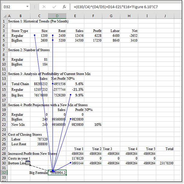
2. Click Trace Precedents again. Excel draws arrows from the precedent cells to the precedents of those cells. These are the second-level precedents of the original cell. Continue clicking Trace Precedents to see additional levels. In this case, practically every cell on the worksheet is a precedent of cell D32.

3. To remove the arrows, use the Remove Arrows icon in the Formula Auditing group.

Tracing Dependents

The Formula Auditing section provides another interesting option besides the ones discussed so far in this chapter. You can use the Formula Auditing section to trace dependents, so you can find all the cells on the current worksheet that depend on the active cell. Before deleting a cell, consider clicking Trace Dependents to determine whether any cells on the current sheet refer to this cell. This prevents many #REF! errors from occurring.

Using the Watch Window

If you have a large spreadsheet, you might want to watch the results of some distant cells. You can use the Watch Window icon in the Formula Auditing section of the Formulas tab to open a floating box called the Watch Window screen. To use the Watch Window screen, follow these steps:

1. Click the Add Watch icon. The Add Watch dialog box appears.

2. In the Add Watch dialog box, specify a cell to watch, as shown in Figure 6.13. After you add several cells, the Watch Window screen floats above your worksheet, showing the current value of each cell that was added to it. The Watch Window screen identifies the current value and the current formula of each watched cell.

   

In theory, this feature can be used to watch a value in a far-off section of the worksheet.

Evaluate a Formula in Slow Motion

Most of the time, Excel calculates formulas in an instant. It can help your understanding of the formula to watch it being calculated in slow motion. If you need to see exactly how a formula is being calculated, follow these steps:

1. Select the cell that contains the formula in which you are interested.

2. On the Formulas tab, in the Formula Auditing group, select Evaluate Formula. The Evaluate Formula dialog box appears, showing the formula. The following component of the formula is highlighted: It is the next section of the formula to be calculated.

3. If desired, click Evaluate to calculate the highlighted portion of the formula.

4. Click Step In to begin a new Evaluate section for the cell references in the underlined portion of the formula. Figure 6.14 shows the Evaluate Formula dialog box after stepping in to the E30 portion of the formula.

   

Evaluating Part of a Formula

When you do not need to evaluate an entire formula, use the F9 feature. Follow these steps to evaluate part of a formula:

1. Use the mouse to select just the desired portion of the formula in the formula bar, as shown in Figure 6.15.

   

2. Press F9. Excel calculates just the highlighted portion of the formula, as shown in Figure 6.16.

   

Be sure to press the Esc key to exit the formula after you use this method. If you press Enter instead to accept the formula, that portion of the formula permanently stays in its calculated form, such as 0.407407.