Chapter 12
Array Formulas and Names in Excel

Long before Microsoft introduced tables and formulas such as =[@Revenue]–[@Cost], spreadsheets have offered the capability to assign a name to a cell, a range of cells, or a formula. The theory is that using a name for a range is easier to understand when used in a formula. For instance, =SUM(MyExpenses) makes formulas more self-documenting than =SUM(Sheet5!AB2:AB99). In Excel 2019, you use the Name Manager interface to assign and use names effectively.

Advantages of Using Names

Names have a variety of uses in a workbook. A name can be applied to any cell or range. Names are also useful for the following:

• Making formulas easier to understand and write. Defined names are offered in the Formula AutoComplete drop-down menu as you start to type a formula.

• Quick navigation.

• Forcing a formula reference to remain absolute—without having to use the dollar sign.

• Doing a two-way lookup with the intersection operator.

• Improving report results from Solver and Scenario Manager.

• Storing a value that will be used repeatedly but that might occasionally need to change, such as a sales tax rate.

• Storing formulas.

• Defining a dynamic range.

You have various ways to name a cell. The easiest way to define a name for a cell is to use the name box. To do so, select any cell in your worksheet. To the left of the formula bar is a box with the address of that cell. This box is known as the name box (see Figure 12.1). The quick way to assign a name is to click inside the name box and type the name, such as Revenue.

When you press Enter, Excel tries to assign the name. If you get no message, the name is valid. If you get the message, “You must enter a valid reference you want to go to, or type a valid name for the selection,” then the name is invalid. If you are taken to a new range, that name already exists.

The following are some basic rules for valid names:

• Names can be up to 255 characters long.

• Names can start with a letter, an underscore, or a backslash. Numbers can be used in a name, but they can’t be the first character in the name.

• Names cannot contain spaces. However, you can use an underscore or a period in a name. For example, the names Gross_Profit and Gross.Profit are valid.

• Names cannot look like cell addresses. ROI2015 is already a cell address. The names R, r, C, and c cannot be used because these are the shorthand for selecting an entire row or column.

• Names cannot contain operator characters such as these:

  + - * / ( ) ^ & < > = %

• Names cannot contain special characters such as these:

  ! " # $ ' , ; : @ [ ] { } ` | ~

• Names cannot start with “c” or “r” followed by numbers and text. For example, r82hello or c123test are not valid. There is no longer a valid reason for this anomaly.

Table 12.1 provides some examples of valid and invalid names.

Naming a Cell by Using the Name Dialog Box

The Formulas tab contains a group called Defined Names. The following example introduces the Name dialog box:

1. Select a cell that you would like to name. Click the Define Name icon from the Formulas tab. The New Name dialog box appears. In Figure 12.2, cell B8 is being assigned a name.

   

2. The New Name box uses IntelliSense to propose a name. Notice that in this particular example, Excel’s IntelliSense was able to ascertain that this cell contains the text Cost of Good Sold. Because that is not a valid name, Excel instead proposed naming the cell Cost_of_Good_Sold. You can either keep that name or override it with a name you prefer. In this case, override that name with the name COGS.

3. For now, leave the scope as Workbook. For a discussion of when to use a worksheet-level scope, see “Avoiding Problems by Using Worksheet-Level Scope,” later in this chapter.

As you can see in Figure 12.3, the name was applied because the name box now shows COGS instead of B8.

Using the Name Box for Quick Navigation

One advantage of using names is that you can use the drop-down menu in the name box to jump to any named cell. This includes cells that might be in distant sections of the worksheet or even on other sheets in the workbook.

If you plan to use the name box for navigation, assign a name to the upper-left corner of each section of your workbook. The name box drop-down menu then provides a mini table of contents, and people can use the name box to jump to any section of the workbook.

To illustrate this concept, follow these steps:

1. Click the New Sheet icon (next to the right-most sheet tab) to add a new sheet to the workbook.

2. On the new sheet, go to a distant cell. Give that cell a name, such as SectionTwo. Return to the original sheet in the workbook.

3. Click the name box’s drop-down menu arrow to access a list of all names in the workbook, as shown in Figure 12.4.

   

4. Choose a name from the list to navigate quickly to that cell, even if it is on another worksheet.

As you can see, named ranges are a great tool for quickly navigating a workbook. Note that names are presented in the name box alphabetically. If you want the names to appear sequentially, you can add names, such as Section1, Section2, Section3, and so on. You can also prefix the section names with letters, such as A-Income, B-Costs, C-Expense, D-Tax, E-Income. Then, you can jump to a section by choosing it from the alphabetical list in the name box. When used in this way, names in Excel are almost like bookmarks in Word.

Avoiding Problems by Using Worksheet-Level Scope

Most names have a workbook-level scope. There are two specific reasons why you might want to use worksheet-level scope instead:

• You have many similar worksheets in a workbook, and you want to define the same names on each sheet. For example, you might want Revenue and COGS on each sheet from January through December.

• You routinely copy a worksheet from one workbook, and you want to avoid having phantom names with #REF! errors appear in the copied sheet. Note that this problem was prevalent before Excel 2013 but has now been corrected.

Defining a Worksheet-Level Name

To declare a name with worksheet-level scope, you can use one of these methods:

• Use Insert, Define Name. In the New Name dialog box, choose Worksheet from the Scope drop-down menu.

• Click in the name box and type Jan!Rev, as shown in Figure 12.5. If the sheet name contains a space, wrap the sheet name in apostrophes: ‘Budget 2018’!Rev.

  

• You will often inadvertently create a worksheet-level name by using a duplicate name. If you define Revenue on the January worksheet without declaring a scope, the name will have a workbook-level scope. If you then define Revenue on the February worksheet, it will automatically have a worksheet-level scope.

Referring to Worksheet-Level Names

If you want to refer to the Rev cell on the January worksheet from anywhere else on the January worksheet, simply use =Rev.

If you want to refer to the Revenue cell on the January worksheet from anywhere else in the workbook, use =Jan!Rev.

Using Named Ranges to Simplify Formulas

As introduced at the start of this chapter, the original reason for having named ranges was to simplify formulas. In theory, it is easier to understand a formula such as =(Revenue-COGS)/Revenue.

Be sure to define the names before entering formulas that refer to those cells. When you create a formula using the mouse or arrow-key method, Excel automatically uses the names in the formula.

In the following example, the worksheet in Figure 12.6 has a name of Revenue assigned to B6 and a name of COGS assigned to B8. Rather than typing =B6-B8 in cell B9, follow these steps to have Excel create a formula using names:

1. Select the cell where the formula should go. In this example, it is cell B9.

2. Type =.

3. Using the mouse, click the first cell in your formula. In this case, it is cell B6.

4. Type -.

5. Using the mouse, click the next cell in your formula. In this case, it is cell B8.

6. Press Enter.

7. Move the cell pointer back to the formula cell and look in the formula bar. You can see that Excel has built the formula =Revenues-COGS, as shown in Figure 12.6. In theory, this formula is self-documenting and easier to understand than =B6-B8.

   

If you prefer to type your formulas, named ranges can also be a timesaver. Say that you start to type =R. Excel displays a drop-down menu offering many functions that start with R, such as RADIANS, RAND, and RANDBETWEEN. Your defined name of Revenue will be in this list of 20 items.

Keep typing. After you type E, the list shortens to four items: RECEIVED, REPLACE, REPT, and Revenue (see Figure 12.7). As you continue typing and type V, the only item in the list is your defined name of Revenue. You can now click Tab to insert this named range into your formula.

Type the minus sign, type COG, and then press Tab to select COGS from the list.

Retroactively Applying Names to Formulas

When you learn the trick that was discussed in the “Using Named Ranges to Simplify Formulas” section, you might start naming all the input cells in your workbook, hoping that all the preexisting formulas will take on the new names. Unfortunately, this does not work automatically.

To make the names become part of existing formulas, you have to use the Apply command. To do this, follow these steps:

1. On the Formulas tab, select the drop-down menu next to Define Name and select Apply Names. The Apply Names dialog box appears.

2. Choose as many names as you want in the Apply Names box. In this example, you should choose at least GrossProfit and TotalExpenses and then click OK. Existing formulas that point to these named cells change to include the cell names in the formula.

Using Names to Refer to Ranges

It is possible to define a name that refers to a larger range of cells. For example, you can select B11:B13 in Figure 12.8 and type a name such as Expenses into the name box.

If you later select Expenses from the name box, your cursor moves to cell B11, and the entire range is selected. Having a name apply to a range allows formulas such as =Sum(Expenses).

Adding Many Names at Once from Existing Labels and Headings

With Excel 2019, you can add many names in a single command, particularly if the names exist as labels or headings adjacent to the cells.

Suppose you have a worksheet with a series of labels in column A and values in column B. One example is shown in Figure 12.9. To do a wholesale assignment of names to the cells in column B, follow these steps:

1. Select the range of labels and the cells to which they refer. In this example, that range is A4:B16.

2. Select Formulas, Defined Names, Create From Selection. Excel displays the Create Names from Selected Range dialog box.

3. Because the row labels are in the left column of the selected range, select Left Column and then click OK, as shown in Figure 12.9.

   

Excel does a fairly good job of assigning the names. Spaces are replaced with underscores to make the names valid. In this example, cell B4 is assigned the name Net_Sales. Cell C8 is assigned the name Cost_of_Good_Sold. In row 12, where the label contains an ampersand (&), Excel replaces the ampersand with an underscore, to form the name G_A_Expenses. Although this is not as meaningful as it could be if you wrote the name yourself, it is still pretty good.

In Excel 2019, you can apply names by using both the row labels and column headings at the same time. In Figure 12.10, the selections in the Create Names From Selected Ranges dialog box mean that nine new names will be added to the workbook. For example, Northeast refers to B2:F2, and Week5 refers to F2:F5.

Using Intersection to Do a Two-Way Lookup

After using Create from Selection in Figure 12.10, the name Southeast applies to the range B3:F3. The name Week5 applies to F2:F5. You can do a two-way lookup by using the intersection operator within the SUM function. The intersection operator is a space. A formula such as =SUM(Week5 Southeast) looks for the intersection of the two ranges and returns the value 1001 from cell F3 (see Figure 12.11). You can leave out the SUM() and simply type =Week5 Southeast.

The formula in Figure 12.11 is significantly easier than a traditional two-way lookup with the following:

Click here to view code image

=INDEX(B2:F5,MATCH("Southeast",$A$2:$A$5,0),MATCH("Week5",$B$1:$F$1,0))

Using Implicit Intersection

In Figures 12.10 through 12.12, the name “Northeast” applies to B2:F2. If you type =Northeast anywhere in columns B:F, Excel uses implicit intersection. Excel assumes that you want to refer only to the portion of the Northeast range that intersects the current column. Typing =Northeast in D7 returns 1031 because of the five values in the Northeast region: The 1031 in D2 intersects with the formula in D7. This is a cool shortcut method.

In Figure 12.12, an identical formula of =Southeast+Northeast is used in B8:F8.

Implicit intersections also work with vertical ranges. Week4 is defined as E2:E5. If you enter =Week4 anywhere in rows 2 through 5, Excel returns the value from the Week4 range that intersects with the row that contains the formula. This allows identical formulas of =Week4+Week5, as shown in H2:H5 of Figure 12.12.

Using a Name to Avoid an Absolute Reference

A common scenario is when a formula such as VLOOKUP is used in a data set to look up data on another worksheet. You might enter a VLOOKUP formula in cell B2 and copy it to hundreds of records. The formula in cell B2 might be =VLOOKUP(A2,'Lookup Table'!A2:B25,2,False). As you copy this formula to row 3, the reference in the second argument incorrectly changes to 'Lookup Table'!A3:B26. When you need the reference to always point to A2:B25, you can add dollar signs to the reference: $A$2:$B$25.

If you will be frequently adding VLOOKUP formulas that will point to 'Lookup Table'!$A$2:$B$25, it can get tedious to continually use the syntax. After all, it is a confusing mix of dollar signs, apostrophes, and exclamation points.

To simplify the VLOOKUP formula, give A2:B25 a name such as ItemLookup. Then, the formula simply becomes =VLOOKUP(A2,ItemLookup,2,False). As you copy the formula down, it continues to point to A2:B25 on the Lookup Table worksheet. Figure 12.13 compares the formula without a name in B2 and the formula with a name in B3.

Using a Name to Hold a Value

So far, all the names defined in this chapter have referred to a cell or a range of cells. It is possible to assign a constant value to a name by using the New Name dialog box. You might do this to hold a value that could possibly change but would likely rarely change, such as a sales tax rate.

To use a name to hold a value, follow these steps:

1. Either click the Define Name icon or the Name Manager icon, and then click New. The New Name dialog box appears.

2. In the Name field of the New Name dialog box, type a name such as Sales_Tax.

3. In the Refers To box, remove any existing cell reference and type the new value, such as =6.5%.

4. Write formulas that refer to the new name, such as Sales_Tax. The formula might be something like =C2*Sales_Tax.

The advantage of using a name to refer to a constant is that if your tax rate changes, you can edit the value defined in the name, and all the formulas in the workbook recalculate. To edit an existing name, click the Name Manager, click the name, and then select Edit Name.

Assigning a Formula to a Name

Although names are traditionally used to refer to cells or constant values, you can use a name to refer to a formula. Look at any name in the Name Manager. The Refers To column starts with an equal sign, which means that named ranges always contain a formula.

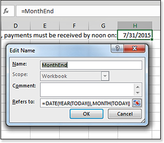
A named formula enables you to replace a complicated formula with an easy-to-remember name. In this basic case, the formula does not contain cell references. For example, suppose you have discovered a fairly complex formula that would be difficult to remember, such as a formula to show the end of this month:

=EOMONTH(TODAY(),0)

In this case, you could assign the formula =EOMONTH(TODAY(),0) to a name such as MonthEnd, as shown in Figure 12.14. You could then use =MonthEnd in any cell to calculate the end of the current month.

Using Power Formula Techniques

Excel offers an amazing variety of formulas. This chapter covers some of the unorthodox formulas you can build in Excel. In this chapter, you discover the following:

• Using a formula to add the same cell across many sheets

• Using a formula to reference the previous sheet

• Editing multiple formulas into one

• Letting data determine the cell reference to use with the INDIRECT function

• Transposing relative column references to rows

• Using ROW() or COLUMN() to return an array of numbers

• Replacing thousands of formulas with one Ctrl+Shift+Enter (CSE) array formula

• Using one formula to return a whole range of answers

Using 3D Formulas to Spear Through Many Worksheets

It is common to have a workbook composed of identical worksheets for each month or quarter of the year. Every worksheet needs to have the same arrangement of rows.

If you want to total a particular cell across all the worksheets, you might try to write a formula with one term for each sheet—for example, =Sheet1!A1+Sheet2!A1+Sheet3!A1.... However, Excel supports a special type of formula that spears through several worksheets to add a particular cell from each worksheet. The syntax of the formula is =SUM(Sheet1:Sheetn!A1). If you use spaces in your worksheet names, add apostrophes around the pair of sheet names =SUM('Jan 2021:Dec2021'!A1).

As shown in Figure 12.15, Net Revenue is in row 4 on the January worksheet and is in the same row on the February worksheet. You cannot see this in Figure 12.15, but the arrangement of rows is identical on every worksheet.

When creating a worksheet, you might be tempted to write a formula such as =Jan!B4+Feb!B4+Mar!B4+Apr!B4, but doing so would be rather tedious.

Instead, you can write a formula that totals cell B4 from each worksheet, Jan through Dec. An example of the formula is =SUM(Jan:Dec!B4). After you enter this formula in cell B4, you can easily copy it to all the other relevant cells in the worksheet, as shown in Figure 12.16.

Excel 2013 introduced a new worksheet function called SHEETS(). You can use =SHEETS(Jan:Dec!A1) to learn that there are 12 sheets in the reference.

=SUM(CostQ1!B4,CostQ2!B4,CostQ3!B4,CostQ4!B4)

Referring to the Previous Worksheet

When you have an arrangement of several sequential worksheets, you might want to keep a running total. This total would be calculated as the total on this sheet plus the running total from the previous sheet.

It is somewhat difficult to build a formula that always points to the previous sheet. Maybe you’ve tried the wrong approach shown in Figure 12.17: On the Feb worksheet, a formula refers to =Jan!B4. However, if you copy the formula to Mar or Apr, the formula still points to the Jan worksheet, which is not what you want.

Excel offers a very cool solution to this problem. The solution requires a few lines of VBA macro code. Don’t be afraid. I can get you there and back without any problems. Here’s what you do:

1. Press Alt+F11 to launch the VBA editor.

2. In the VBA editor, select Insert, Module.

3. Type the following lines into the blank module:

   Click here to view code image

   Function PrevSheet(ByVal MyCell As Range)
    Application.Volatile
    On Error Resume Next
    PrevSheet = Sheets(MyCell.Parent.Index - 1).Range(MyCell.Address)
   End Function

4. Your screen should look similar to Figure 12.18.

   

5. Select File, Close, and Return to Microsoft Excel to return to Excel.

To realize the power of this function, you can put the workbook in Group mode and enter the function in 11 worksheets at once:

1. Select the Feb worksheet.

2. Hold down the Shift key while clicking the Dec worksheet tab. This highlights all 11 worksheets. Although you see the Feb worksheet, anything you do on that worksheet is also done to all 11 selected worksheets.

3. In cell E4, enter =PrevSheet(B4). Press Enter to accept the formula. The Feb worksheet picks up the value from Jan, but each additional worksheet picks up the value from the previous sheet, as shown in Figure 12.19.

   

4. With the worksheets still in Group mode, copy cell B4 from the Feb worksheet to cells B5, B7, and so on.

5. Right-click any sheet tab and select Ungroup.

Combining Multiple Formulas into One Formula

With more than 460 functions available in Excel, it is possible to perform just about any calculation. Many times, however, it is easier to break the task down into many subformulas as you try to solve the problem.

For example, fellow Excel MVP and guru Bob Umlas taught me that I could use the Substitute function to locate the last space in a word. This is handy for finding the last word in a sentence or name. However, unlike Bob, I always need to build this formula over the course of several columns. It takes me seven columns to do a trick that Bob can do in one. Figure 12.20 shows all the formulas used to replicate the trick.

If you’ve ever built a formula in small steps as shown previously, you can begin consolidating the formulas into one monster formula.

However, there’s an easier way to combine many formulas into one formula. As an example, follow these steps:

1. Examine the final formula. It references cells that contain one or more subformulas. In Figure 12.21, cell H2 has a formula that references the value in A2 and subformulas in G2, C2, and G2. You remove the reference to G2 first.

   

2. Move the cell pointer to the subformula in G2.

3. Press F2 to put the formula in edit mode.

4. With the mouse, highlight the formula in the formula bar, but do not highlight the equal sign in the subformula (see Figure 12.22).

   

5. Press Ctrl+C to copy this portion of the subformula to the Clipboard.

6. Go back to the final formula. Press F2 to put the formula in edit mode.

7. In the formula bar, using the mouse, highlight the first instance of G2, as shown in Figure 12.23.

   

8. Press Ctrl+V to paste the subformula from cell G2 in place of the letters G2. The formula appears as shown in Figure 12.24. Note that you just added a new reference to the F2 subformula.

   

9. Because G2 appears again in this formula, repeat steps 7 and 8 for the second instance of G2.

10. Press Enter to accept this intermediate formula of =MID(A2,FIND("!",F2)+1, C2-FIND("!",F2)).

11. If there are additional references to a cell with a subformula in the new formula, repeat steps 1–10 for the next reference. In this case, you would replace the characters F2 with SUBSTITUTE(A2," ","!",E2). Continue working through the formula, replacing E2, then D2, then C2, then B2. Eventually, you end up with a monster formula, as shown in Figure 12.25. Your co-workers will look at that formula and assume you must be a spreadsheet wizard like Excel MVP Bob Umlas.

    

Turning a Range of Formulas on Its Side

The Transpose option in the Paste Options dialog box is great for changing values that span across several columns into values that go down a column. Here’s an example:

1. In Figure 12.26, you select B1:M1 and then press Ctrl+C.

   

2. Select the top-left cell where the range should be copied. In this example, select cell A7.

3. Right-click in the Paste Options section and select Transpose, as shown in Figure 12.26. The month names now go down the row. However, there’s no good way to copy the calculation for profit from row 4 to the new table. You normally have to enter 12 different formulas in the range B7:B17, as shown in Figure 12.27.

   

However, there are two ways to easily enter a single formula that turns those results on their side.

First, you can use the INDEX function in conjunction with ROW. Try it:

1. In cell B7, enter =ROW(1:1). The result is the number 1.

2. Copy the formula from cell B7 down to B7:B18. The result returns a string of integers from 1 through 12.

3. Use the formula =ROW(A1) as the second argument in the INDEX function. A formula of =INDEX($B$4:$M$4,0,ROW(1:1)) achieves the perfect result, as shown in Figure 12.28.

   

One danger exists with just about every method described in this chapter: They produce results that the average person does not understand. So if you want to end up with straightforward formulas in B7:B18, you can use the following method:

1. Enter a formula, such as =B4, in cell B5.

2. Copy the first formula across row 5 for each month.

3. Highlight the formulas in B5:M5.

4. Use Home, Editing, Find & Select, Replace to display the Find And Replace dialog box. In the Find What box, enter an equal sign. In the Replace With box, enter an exclamation point. Click Replace All to change every occurrence of = to !. This converts the formulas to text, as shown in row 5 of Figure 12.29.

   

5. Copy the range and highlight a new cell (in this example, cell B7).

6. Right-click and select Transpose. Because the cells are all text, they transpose perfectly, as shown in B7:B18 of Figure 12.29.

7. Use Ctrl+H or Home, Editing, Find & Select, Replace to display the Find And Replace dialog box. Type an exclamation point in Find What and an equal sign in Replace With. Click Replace All to change every ! back to =. It now looks as if you actually typed all 12 formulas individually.

Coercing a Range of Dates Using an Array Formula

A wildly powerful type of formula exists that most Excel users have never experienced. This single formula can do thousands of calculations. The formula is known as an array formula. You must use Ctrl+Shift+Enter when entering an array formula to tell Excel to evaluate the formula as an array.

Note: The Ctrl+Shift+Enter formula discussed in this section applies only to Excel 2019. Customers using Office 365 can use dynamic arrays to replace this formula. In a dynamic array, using SEQUENCE((C2-C1+1),1,C1,2) will replace using ROW(INDIRECT(C1&" "&C2)) in the following example. Ctrl+Shift+Enter will not be required.

Suppose you want to find out how many Wednesdays occurred between two dates. Enter the starting and ending dates in cells in an Excel worksheet, as shown in Figure 12.30.

To start, the WEEKDAY function returns a number from 1 to 7 corresponding to the day of the week. =WEEKDAY(C1) returns the number 4 if the day is a Wednesday.

To check to see whether a particular day is a Wednesday, use the IF function:

=IF(WEEKDAY(C1)=4,1,0)

Using that formula, you could build a table showing all dates from the beginning date to the ending date as rows. The second column uses the IF/WEEKDAY function to test whether each date is a Wednesday. Sum that column to count the Wednesdays in the range. However, this table will contain hundreds of rows for every year in the data range.

Instead, use ROW(INDIRECT(C1&":"&C2)) to build an array in memory of all the dates. Although cell C1 is displaying 6/30/2015, it actually contains the number 42185. Similarly, cell C2 contains the number 43358. Concatenating C1 with a colon and C2 builds a text string of “42185:43358”. This text is a valid reference, pointing to all the rows from 42185 to 43358. Asking for the ROW of that reference returns an array with the numbers 42185 to 43358.

To build the array formula, replace “C1” in the original IF/WEEKDAY function with the ROW/INDIRECT functions:

Click here to view code image

=IF(WEEKDAY(ROW(INDIRECT(C1&":"&C2)))=4,1,0)

That formula returns a series of zeroes and ones. Because you want to add up the ones in the resulting array, wrap the formula in a SUM function:

Click here to view code image

=SUM(IF(WEEKDAY(ROW(INDIRECT(C1&":"&C2)))=4,1,0))

After you type that formula, press Ctrl+Shift+Enter. Excel calculates hundreds of intermediate results and shows the answer in a single cell.

To learn more about Array formulas, check out Mike Girvin’s Ctrl+Shift+Enter book (ISBN 978-1-61547-007-5). Office 365 customers will have access to new modern array functions such as SEQUENCE. You can simplify the above formula with =SUM(IF(WEEKDAY(SEQUENCE(C1,(C2-C1+1)))=4,1,0)), and this will require no Ctrl+Shift+Enter. Read about these in Chapter 1, under “New Array Functions in Office 365.”

Troubleshooting

Array formulas are difficult to paste. The paste area cannot overlap with the copy area.

In the following figure, the array formula in D5 needs to be copied to D5:J35.

Normally, you would copy Cell D5 and then paste to cells D5:J35. With array formulas, this leads to an error. If you attempt to do this, you are told that you cannot move or change part of an array. The solution is to do the copy in two pieces:

1. Copy Cell D5 to D6:D35.

2. Copy D5:D35 and paste it to E5:J35.