
Geometry Representation and Modeling
Two principal tasks are required to create an image of a three-dimensional scene: modeling and rendering. The modeling task generates a model, which is the description of an object that is going to be used by the graphics system. Models must be created for every object in a scene; they should accurately capture the geometric shape and appearance of the object. Some or all of this task commonly occurs when the application is being developed, by creating and storing model descriptions as part of the application’s data.
The second task, rendering, takes models as input and generates pixel values for the final image. OpenGL is principally concerned with object rendering; it does not provide explicit support for creating object models. The model input data is left to the application to provide. The OpenGL architecture is focused primarily on rendering polygonal models; it doesn’t directly support more complex object descriptions, such as implicit surfaces. Because polygonal models are the central manner in which to define an object with OpenGL, it is useful to review the basic ideas behind polygonal modeling and how they relate to it.
1.1 Polygonal Representation
OpenGL supports a handful of primitive types for modeling two-dimensional (2D) and three-dimensional (3D) objects: points, lines, triangles, quadrilaterals, and (convex) polygons. In addition, OpenGL includes support for rendering higher-order surface patches using evaluators. A simple object, such as a box, can be represented using a polygon for each face in the object. Part of the modeling task consists of determining the 3D coordinates of each vertex in each polygon that makes up a model. To provide accurate rendering of a model’s appearance or surface shading, the modeler may also have to determine color values, shading normals, and texture coordinates for the model’s vertices and faces.
Complex objects with curved surfaces can also be modeled using polygons. A curved surface is represented by a gridwork or mesh of polygons in which each polygon vertex is placed on a location on the surface. Even if its vertices closely follow the shape of the curved surface, the interior of the polygon won’t necessarily lie on the surface. If a larger number of smaller polygons are used, the disparity between the true surface and the polygonal representation will be reduced. As the number of polygons increases, the approximation improves, leading to a trade-off between model accuracy and rendering overhead.
When an object is modeled using polygons, adjacent polygons may share edges. To ensure that shared edges are rendered without creating gaps between them, polygons that share an edge should use identical coordinate values at the edge’s endpoints. The limited precision arithmetic used during rendering means edges will not necessarily stay aligned when their vertex coordinates are transformed unless their initial values are identical. Many data structures used in modeling ensure this (and save space) by using the same data structure to represent the coincident vertices defining the shared edges.
1.2 Decomposition and Tessellation
Tessellation refers to the process of decomposing a complex surface, such as a sphere, into simpler primitives such as triangles or quadrilaterals. Most OpenGL implementations are tuned to process triangles (strips, fans, and independents) efficiently. Triangles are desirable because they are planar and easy to rasterize unambiguously. When an OpenGL implementation is optimized for processing triangles, more complex primitives such as quad strips, quads, and polygons are decomposed into triangles early in the pipeline.
If the underlying implementation is performing this decomposition, there is a performance benefit in performing it a priori, either when the database is created or at application initialization time, rather than each time the primitive is issued. Another advantage of having the application decompose primitives is that it can be done consistently and independently of the OpenGL implementation. OpenGL does not specify a decomposition algorithm, so different implementations may decompose a given quadrilateral or polygon differently. This can result in an image that is shaded differently and has different silhouette edges when drawn on two different OpenGL implementations. Most OpenGL implementations have simple decomposition algorithms. Polygons are trivially converted to triangle fans using the same vertex order and quadrilaterals are divided into two triangles; one triangle using the first three vertices and the second using the first plus the last two vertices.
These simple decomposition algorithms are chosen to minimize computation overhead. An alternative is to choose decompositions that improve the rendering quality. Since shading computations assume that a primitive is flat, choosing a decomposition that creates triangles with the best match of the surface curvature may result in better shading. Decomposing a quad to two triangles requires introducing a new edge along one of the two diagonals.
A method to find the diagonal that results in more faithful curvature is to compare the angles formed between the surface normals at diagonally opposing vertices. The angle measures the change in surface normal from one corner to its opposite. The pair of opposites forming the smallest angle between them (closest to flat) is the best candidate diagonal; it will produce the flattest possible edge between the resulting triangles, as shown in Figure 1.1. This algorithm may be implemented by computing the dot product between normal pairs, then choosing the pair with the largest dot product (smallest angle). If surface normals are not available, then normals for a vertex may be computed by taking the cross products of the two vectors with origins at that vertex. Surface curvature isn’t the only quality metric to use when decomposing quads. Another one splits the quadrilateral into triangles that are closest to equal in size.
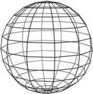
Tessellation of simple surfaces such as spheres and cylinders is not difficult. Most implementations of the OpenGL Utility (GLU) library use a straightforward latitude-longitude tessellation for a sphere. While this algorithm is easy to implement, it has the disadvantage that the quads produced from the tessellation have widely varying sizes, as shown in Figure 1.2. The different sized quads can cause noticeable artifacts, particularly if the object is lighted and rotating.
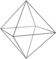
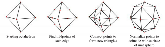
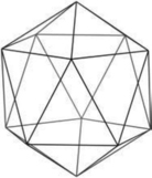
A better algorithm generates triangles with sizes that are more consistent. Octahedral and icosahedral tessellations work well and are not very difficult to implement. An octahedral tessellation starts by approximating a sphere with a single octahedron whose vertices are all on the unit sphere, as shown in Figure 1.3. Since each face of the octahedron is a triangle, they can each be easily split into four new triangles.
Each triangle is split by creating a new vertex in the middle of each of the triangle’s existing edges, then connecting them, forming three new edges. The result is that four new triangles are created from the original one; the process is shown in Figure 1.4. The coordinates of each new vertex are divided by the vertex’s distance from the origin, normalizing them. This process scales the new vertex so that it lies on the surface of the unit sphere. These two steps can be repeated as desired, recursively dividing all of the triangles generated in each iteration.
The same algorithm can be used with an icosahedron as the base object, as shown in Figure 1.5, by recursively dividing all 20 sides. With either algorithm, it may not be optimal to split the triangle edges in half when tesselating. Splitting the triangle by other amounts, such as by thirds, or even an arbitrary number, may be necessary to produce a uniform triangle size when the tessellation is complete. Both the icosahedral and octahedral algorithms can be coded so that triangle strips are generated instead of independent triangles, maximizing rendering performance. Alternatively, indexed independent triangle lists can be generated instead. This type of primitive may be processed more efficiently on some graphics hardware.
1.3 Shading Normals
OpenGL computes surface shading by evaluating lighting equations at polygon vertices. The most general form of the lighting equation uses both the vertex position and a vector that is normal to the object’s surface at that position; this is called the normal vector. Ideally, these normal vectors are captured or computed with the original model data, but in practice there are many models that do not include normal vectors.
Given an arbitrary polygonal model without precomputed normals, it is easy to generate polygon normals for faceted shading, but a bit more difficult to create correct vertex normals when smooth shading is desired. Computing the cross-product of two edges,
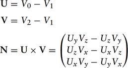
then normalizing the result,
yields a unit-length vector, N′, called a facet normal. Figure 1.6 shows the vectors to use for generating a triangle’s cross product (assuming counterclockwise winding for a front-facing surface).
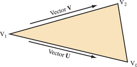
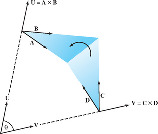
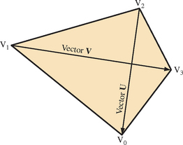
Computing the facet normal of a polygon with more than three vertices is more difficult. Often such polygons are not perfectly planar, so the result may vary depending on which three vertices are used. If the polygon is a quadrilateral, one good method is to take the cross product of the vectors between opposing vertices. The two diagonal vectors U = V0 − V2 and V = V3 − V1 used for the cross product are shown in Figure 1.7.
For polygons with more than four vertices it can be difficult to choose the best vertices to use for the cross product. One method is to to choose vertices that are the furthest apart from each other, or to average the result of several vertex cross products.
1.3.1 Smooth Shading
To smoothly shade an object, a given vertex normal should be used by all polygons that share that vertex. Ideally, this vertex normal is the same as the surface normal at the corresponding point on the original surface. However, if the true surface normal isn’t available, the simplest way to approximate one is to add all (normalized) normals from the common facets then renormalize the result (Gouraud, 1971). This provides reasonable results for surfaces that are fairly smooth, but does not look good for surfaces with sharp edges.
In general, the polygonal nature of models can be hidden by smoothing the transition between adjacent polygons. However, an object that should have hard edges, such as a cube, should not have its edges smoothed. If the model doesn’t specify which edges are hard, the angle between polygons defining an edge, called the crease angle, may be used to distinguish hard edges from soft ones.
The value of the angle that distinguishes hard edges from soft can vary from model to model. It is fairly clear that a 90-degree angle nearly always defines a hard edge, but the best edge type for a 45-degree crease angle is less clear. The transition angle can be defined by the application for tuning to a particular model; using 45 degrees as a default value usually produces good results.
The angle between polygons is determined using the dot product of the unit-length facet normals. The value of the dot product is equal to the cosine of the angle between the vectors. If the dot product of the two normals is greater than the cosine of the desired crease angle, the edge is considered soft, otherwise it is considered hard. A hard edge is created by generating separate normals for each side of the edge. Models commonly have a mixture of both hard and soft edges, and a single edge may transition from hard to soft. The remaining normals common to soft edges should not be split to ensure that those soft edges retain their smoothness.
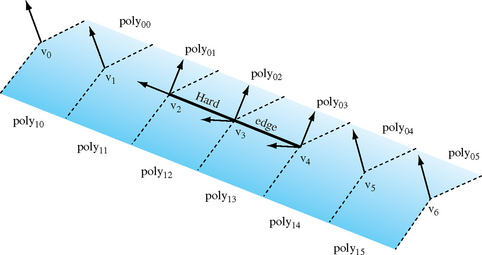
Figure 1.8 shows an example of a mesh with two hard edges in it. The three vertices making up these hard edges, v2, v3, and v4, need to be split using two separate normals. In the case of vertex v4, one normal would be applied to poly02 and poly03 while a different normal would apply to poly12 and poly13. This ensures that the edge between poly02 and poly03 looks smooth while the edge between poly03 and poly13 has a distinct crease. Since v5 is not split, the edge between poly04 and poly14 will look sharper near v4 and will become smoother as it gets closer to v5. The edge between v5 and v6 would then be completely smooth. This is the desired effect.
For an object such as a cube, three hard edges will share one common vertex. In this case the edge-splitting algorithm needs to be repeated for the third edge to achieve the correct results.
1.3.2 Vertex Winding Order
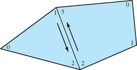
Some 3D models come with polygons that are not all wound in a clockwise or counterclockwise direction, but are a mixture of both. Since the polygon winding may be used to cull back or front-facing triangles, for performance reasons it is important that models are made consistent; a polygon wound inconsistently with its neighbors should have its vertex order reversed. A good way to accomplish this is to find all common edges and verify that neighboring polygon edges are drawn in the opposite order (Figure 1.9).
To rewind an entire model, one polygon is chosen as the seed. All neighboring polygons are then found and made consistent with it. This process is repeated recursively for each reoriented polygon until no more neighboring polygons are found. If the model is a single closed object, all polygons will now be consistent. However, if the model has multiple unconnected pieces, another polygon that has not yet been tested is chosen and the process repeats until all polygons are tested and made consistent.
To ensure that the rewound model is oriented properly (i.e., all polygons are wound so that their front faces are on the outside surface of the object), the algorithm begins by choosing and properly orienting the seed polygon. One way to do this is to find the geometric center of the object: compute the object’s bounding box, then compute its mid-point. Next, select a vertex that is the maximum distance from the center point and compute a (normalized) out vector from the center point to this vertex. One of the polygons using that vertex is chosen as the seed. Compute the normal of the seed polygon, then compute the dot product of the normal with the out vector. A positive result indicates that seed is oriented correctly. A negative result indicates the polygon’s normal is facing inward. If the seed polygon is backward, reverse its winding before using it to rewind the rest of the model.
1.4 Triangle Stripping
One of the simplest ways to speed up an OpenGL program while simultaneously saving storage space is to convert independent triangles or polygons into triangle strips. If the model is generated directly from NURBS data or from some other regular geometry, it is straightforward to connect the triangles together into longer strips. Decide whether the first triangle should have a clockwise or counterclockwise winding, then ensure all subsequent triangles in the list alternate windings (as shown in Figure 1.10). Triangle fans must also be started with the correct winding, but all subsequent triangles are wound in the same direction (Figure 1.11).
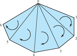
Since OpenGL does not have a way to specify generalized triangle strips, the user must choose between GL_TRIANGLE_STRIP and GL_TRIANGLE_FAN. In general, the triangle strip is the more versatile primitive. While triangle fans are ideal for large convex polygons that need to be converted to triangles or for triangulating geometry that is cone-shaped, most other cases are best converted to triangle strips.
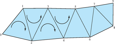
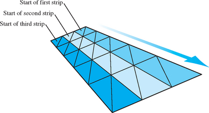
For regular meshes, triangle strips should be lined up side by side as shown in Figure 1.12. The goal here is to minimize the number of total strips and try to avoid “orphan” triangles (also known as singleton strips) that cannot be made part of a longer strip. It is possible to turn a corner in a triangle strip by using redundant vertices and degenerate triangles, as described in Evans et al. (1996).
1.4.1 Greedy Tri-stripping
A fairly simple method of converting a model into triangle strips is often known as greedy tri-stripping. One of the early greedy algorithms, developed for IRIS GL,1 allowed swapping of vertices to create direction changes to the facet with the least neighbors. In OpenGL, however, the only way to get behavior equivalent to swapping vertices is to repeat a vertex and create a degenerate triangle, which is more expensive than the original vertex swap operation was.
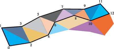
For OpenGL, a better algorithm is to choose a polygon, convert it to triangles, then move to the polygon which has an edge that is shared with the last edge of the previous polygon. A given starting polygon and starting edge determines the strip path. The strip grows until it runs off the edge of the model or reaches a polygon that is already part of another strip (Figure 1.13). To maximize the number of triangles per strip, grow the strip in both directions from starting polygon and edge as far as possible.
A triangle strip should not cross a hard edge, since the vertices on that edge must be repeated redundantly. A hard edge requires different normals for the two triangles on either side of that edge. Once one strip is complete, the best polygon to choose for the next strip is often a neighbor to the polygon at one end or the other of the previous strip. More advanced triangulation methods do not try to keep all triangles of a polygon together. For more information on such a method refer to Evans et al. (1996).
1.5 Vertices and Vertex Arrays
In addition to providing several different modeling primitives, OpenGL provides multiple ways to specify the vertices and vertex attributes for each of the primitive types. There are two reasons for this. The first is to provide flexibility, making it easier to match the way the model data is transferred to the OpenGL pipeline with the application’s representation of the model (data structure). The second reason is to create a more compact representation, reducing the amount of data sent to the graphics accelerator to generate the image–less data means better performance.
For example, an application can render a sphere tessellated into individual (independent) triangles. For each triangle vertex, the application can specify a vertex position, color, normal vector, and one or more texture coordinates. Furthermore, for each of these attributes, the application chooses how many components to send (2 (x, y), 3 (x, y, z), or 4 (x, y, z, w) positions, 3 (r, g, b), or 4 (r, g, b, a) colors, and so on) and the representation for each component: short integer, integer, single-precision floating-point, double-precision floating-point.
If the application writer is not concerned about performance, they may always specify all attributes, using the largest number of components (3 component vertices, 4 component colors, 3 component texture coordinates, etc.), and the most general component representation. Excess vertex data is not a problem; in OpenGL it is relatively straightforward to ignore unnecessary attributes and components. For example, if lighting is disabled (and texture generation isn’t using normals), then the normal vectors are ignored. If three component texture coordinates are specified, but only two component texture maps are enabled, then the r coordinate is effectively ignored. Similarly, effects such as faceted shading can be achieved by enabling flat shading mode, effectively ignoring the extra vertex normals.
However, such a strategy hurts performance in several ways. First, it increases the amount of memory needed to store the model data, since the application may be storing attributes that are never used. Second, it can limit the efficiency of the pipeline, since the application must send these unused attributes and some amount of processing must be performed on them, if only to ultimately discard them. As a result, well written and tuned applications try to eliminate any unused or redundant data.
In the 1.1 release of the OpenGL specification, an additional mechanism for specifying vertices and vertex attributes, called vertex arrays, was introduced. The reason for adding this additional mechanism was to improve performance; vertex arrays reduce the number of function calls required by an application to specify a vertex and its attributes. Instead of calling a function to issue each vertex and attribute in a primitive, the application specifies a pointer to an array of attributes for each attribute type (position, color, normal, etc.). It can then issue a single function call to send the attributes to the pipeline. To render a cube as 12 triangles (2 triangles × 6 faces) with a position, color, and normal vector requires 108 (12 triangles × 3 vertices/triangle × 3 attributes/vertex) function calls. Using vertex arrays, only 4 function calls are needed, 3 to set the vertex, color, and normal array addresses and 1 to draw the array (2 more if calls to enable the color and normal arrays are also included). Alternatively, the cube can be drawn as 6 triangle strips, reducing the number of function calls to 72 for the separate attribute commands, while increasing the number of calls to 6 for vertex arrays.
There is a catch, however. Vertex arrays require all attributes to be specified for each vertex. For the cube example, if each face of the cube is a different color, using the the function-per-attribute style (called the fine grain calls) results in 6 calls to the color function (one for each face). For vertex arrays, 36 color values must be specified, since color must be specified for each vertex. Furthermore, if the number of vertices in the primitive is small, the overhead in setting up the array pointers and enabling and disabling individual arrays may outweigh the savings in the individual function calls (for example, if four vertex billboards are being drawn). For this reason, some applications go to great lengths to pack multiple objects into a single large array to minimize the number of array pointer changes. While such an approach may be reasonable for applications that simply draw the data, it may be unreasonable for applications that make frequent changes to it. For example, inserting or removing vertices from an object may require extra operations to shuffle data within the array.
1.5.1 Vertex Buffer Objects
The mechanisms for moving geometry and texture data to the rendering pipeline continue to be an area of active development. One of the perennial difficulties in achieving good performance on modern accelerators is moving geometry data into the accelerator. Usually the accelerator is attached to the host system via a high speed bus. Each time a vertex array is drawn, the vertex data is retrieved from application memory and processed by the pipeline. Display lists offer an advantage in that the opaque representation allows the data to be moved closer to the accelerator, including into memory that is on the same side of the bus as the accelerator itself. This allows implementations to achieve high-performance display list processing by exploiting this advantage.
Unfortunately with vertex arrays it is nearly impossible to use the same technique, since the vertex data is created and managed in memory in the application’s address space (client memory). In OpenGL 1.5, vertex buffer objects were added to the specification to enable the same server placement optimizations that are used with display lists. Vertex buffer objects allow the application to allocate vertex data storage that is managed by the OpenGL implementation and can be allocated from accelerator memory. The application can store vertex data to the buffer using an explicit transfer command (glBufferData), or by mapping the buffer (glMapBuffer). The vertex buffer data can also be examined by the application allowing dynamic modification of the data, though it may be slower if the buffer storage is now in the accelerator. Having dynamic read-write access allows geometric data to be modified each frame, without requiring the application to maintain a separate copy of the data or explicitly copy it to and from the accelerator. Vertex buffer objects are used with the vertex array drawing commands by binding a vertex buffer object to the appropriate array binding point (vertex, color, normal, texture coordinate) using the array point commands (for example, glNormalPointer). When an array has a bound buffer object, the array pointer is interpreted relative to the buffer object storage rather than application memory addresses.
Vertex buffer objects do create additional complexity for applications, but they are needed in order to achieve maximum rendering performance on very fast hardware accelerators. Chapter 21 discusses additional techniques and issues in achieving maximum rendering performance from an OpenGL implementation.
1.5.2 Triangle Lists
Most of this chapter has emphasized triangle strips and fans as the optimal performing primitive. It is worth noting that in some OpenGL implementations there are other triangle-based representations that perform well and have their own distinct advantages. Using the glDrawElements command with independent triangle primitives (GL_TRIANGLES), an application can define lists of triangles in which vertices are shared. A vertex is shared by reusing the index that refers to it. Triangle lists have the advantage that they are simple to use and promote the sharing of vertex data; the index is duplicated in the index list, rather than the actual triangle.
In the past, hardware accelerators did not process triangle lists well. They often transformed and lit a vertex each time it was encountered in the index list, even if it had been processed earlier. Modern desktop accelerators can cache transformed vertices and reuse them if the indices that refer to them are “close together” in the array. More details of the underlying implementation are described in Section 8.2. With these improvements in implementations, triangle lists are a viable high-performance representation. It is often still advantageous to use strip and fan structures, however, to provide more optimization opportunities to the accelerator.
1.6 Modeling vs. Rendering Revisited
This chapter began by asserting that OpenGL is primarily concerned with rendering, not modeling. The interactivity of an application, however, can range from displaying a single static image, to interactively creating objects and changing their attributes dynamically. The characteristics of the application have a fundamental influence on how their geometric data is represented, and how OpenGL is used to render the data. When speed is paramount, the application writer may go to extreme lengths to optimize the data representation for efficient rendering. Such optimizations may include the use of display lists and vertex arrays, pre-computing the lighted color values at each vertex, and so forth. However, a modeling application, such as a mechanical design program, may use a more general representation of the model data: double-precision coordinate representation, full sets of colors and normals for each vertex. Furthermore, the application may re-use the model representation for non-rendering purposes, such as collision detection or finite element computations.
There are other possibilities. Many applications use multiple representations: they start with a single “master” representation, then generate subordinate representations tuned for other purposes, including rendering, collision detection, and physical model simulations. The creation of these subordinate representations may be scheduled using a number of different techniques. They may be generated on demand then cached, incrementally rebuilt as needed, or constructed over time as a background task. The method chosen depends on the needs of the application.
The key point is that there isn’t a “one size fits all” recipe for representing model data in an application. One must have a thorough understanding of all of the requirements of the application to find the representation and rendering strategy that best suits it.
1Silicon Graphics’ predecessor to OpenGL.