In this section, I will use the data in the table called geo1, which was created in the last section for a map display. It was made to create a simple dashboard, and publish the dashboard to an external client. From the Workspace menu, I have created a new dashboard called dash1. If I edit the controls tab of this dashboard, I can start to enter SQL, and create graphs, as shown in the following screenshot. Each graph is represented as a view and can be defined via SQL. It can be resized, and configured using the plot options as per the individual graphs. Use the Add drop-down menu to add a view. The following screenshot shows that view1 is already created, and added to dash1. view2 is being defined.

Once all the views have been added, positioned, and resized, the edit tab can be selected to present the finalized dashboard. The following screenshot now shows the finalized dashboard called dash1 with three different graphs in different forms, and segments of the data:

This is very useful for giving a view of the data, but this dashboard is within the Databricks cloud environment. What if I want a customer to see this? There is a publish menu option in the top-right part of the dashboard screen, which allows you to publish the dashboard. This displays the dashboard under a new publicly published URL, as shown in the following screenshot. Note the new URL at the top of the following screenshot. You can now share this URL with your customers to present results. There are also options to periodically update the display to represent updates in the underlying data.

This gives you an idea of the available display options. All of the reports, and dashboards created so far have been based upon SQL, and the data returned. In the next section, I will show that reports can be created programmatically using a Scala-based Spark RDD, and streamed data.

The following Scala-based example uses a user-defined class type called birdType, based on the bird name, and the volume encountered. An RDD is created of the bird type records, and then converted into a data frame. The data frame is then displayed. Databricks allows the displayed data to be presented as a table or using plot options as a graph. The following image shows the Scala that is used:

The bar graph, which this Scala example allows to be created, is shown in the following screenshot. The previous Scala code and the following screenshot are less important than the fact that this graph has been created programmatically using a data frame:

This opens up the possibility of programmatically creating data frames, and temporary tables from calculation-based data sources. It also allows for streamed data to be processed, and the refresh functionality of dashboards to be used, to constantly present a window of streamed data. The next section will examine a stream-based example of report generation.

In this section, I will use Databricks capability to upload a JAR-based library, so that we can run a Twitter-based streaming Apache Spark example. In order to do this, I must first create a Twitter account, and a sample application at: https://apps.twitter.com/.

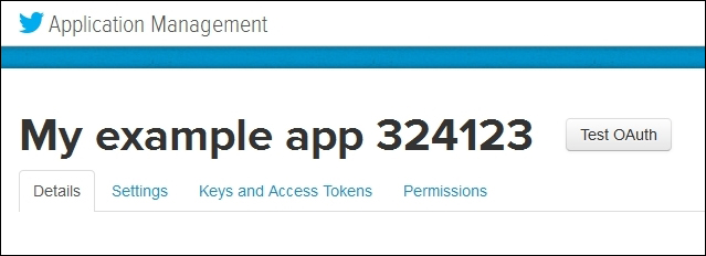
The following screenshot shows that I have created an application called My example app. This is necessary, because I need to create the necessary access keys, and tokens to create a Scala-based twitter feed.

If I now select the application name, I can see the application details. This provides a menu option, which provides access to the application details, settings, access tokens, and permissions. There is also a button which says Test OAuth, this enables the access and token keys that will be created to be tested. The following screenshot shows the application menu options:

By selecting the Keys and Access Tokens menu option, the access keys, and the access tokens can be generated for the application. Each of the application settings and tokens, in this section, have an API key, and a secret key. The top of the form, in the following screenshot, shows the consumer key, and consumer secret (of course, the key and account details have been removed from these images for security reasons).

There are also options in the previous screenshot to regenerate the keys, and set permissions. The next screenshot shows the application access token details. There is an access token, and an access token secret. It also has the options to regenerate the values, and revoke access:

Using these four alpha numeric value strings, it is possible to write a Scala example to access a Twitter stream. The values that will be needed are as follows:

In the following code sample, I will remove my own key values for security reasons. You just need to add your own values to get the code to work. I have developed my library, and run the code locally to check whether it will work. I did this before loading it to Databricks, in order to reduce time, and costs due to debugging. My Scala code sample looks like the following code. First, I define a package, import Spark streaming, and twitter resources. Then, I define an object class called twitter1, and create a main function:

package nz.co.semtechsolutions

import org.apache.spark._
import org.apache.spark.SparkContext._
import org.apache.spark.streaming._
import org.apache.spark.streaming.twitter._
import org.apache.spark.streaming.StreamingContext._
import org.apache.spark.sql._
import org.apache.spark.sql.types.{StructType,StructField,StringType}

object twitter1 {

  def main(args: Array[String]) {

Next, I create a Spark configuration object using an application name. I have not used a Spark master URL, as I will let both, spark-submit, and Databricks assign the default URL. From this, I will create a Spark context, and define the Twitter consumer, and access values:

    val appName = "Twitter example 1"
    val conf    = new SparkConf()

    conf.setAppName(appName)
    val sc = new SparkContext(conf)

    val consumerKey       = "QQpl8xx"
    val consumerSecret    = "0HFzxx"
    val accessToken       = "323xx"
    val accessTokenSecret = "Ilxx"

I set the Twitter access properties using the System.setProperty call, and use it to set the four twitter4j oauth access properties using the access keys, which were generated previously:

    System.setProperty("twitter4j.oauth.consumerKey", consumerKey)
    System.setProperty("twitter4j.oauth.consumerSecret",
       consumerSecret)
    System.setProperty("twitter4j.oauth.accessToken", accessToken)
    System.setProperty("twitter4j.oauth.accessTokenSecret",
       accessTokenSecret)

A streaming context is created from the Spark context, which is used to create a Twitter-based Spark DStream. The stream is split by spaces to create words, and it gets filtered by the words starting with #, to select hash tags:

    val ssc    = new StreamingContext(sc, Seconds(5) )
    val stream = TwitterUtils.createStream(ssc,None)
       .window( Seconds(60) )

    // split out the hash tags from the stream

    val hashTags = stream.flatMap( status => status.getText.split(" ").filter(_.startsWith("#")))

The function used below to get a singleton SQL Context is defined at the end of this example. So, for each RDD in the stream of hash tags, a single SQL context is created. This is used to import implicits which allows an RDD to be implicitly converted to a data frame using toDF. A data frame is created from each rdd called dfHashTags, and this is then used to register a temporary table. I have then run some SQL against the table to get a count of rows. The count of rows is then printed. The horizontal banners in the code are just used to enable easier viewing of the output of results when using spark-submit:

hashTags.foreachRDD{ rdd =>

val sqlContext = SQLContextSingleton.getInstance(rdd.sparkContext)
import sqlContext.implicits._

val dfHashTags = rdd.map(hashT => hashRow(hashT) ).toDF()

dfHashTags.registerTempTable("tweets")

val tweetcount = sqlContext.sql("select count(*) from tweets")

println("
============================================")
println(  "============================================
")

println("Count of hash tags in stream table : "
   + tweetcount.toString )

tweetcount.map(c => "Count of hash tags in stream table : "
   + c(0).toString ).collect().foreach(println)

println("
============================================")
println(  "============================================
")

} // for each hash tags rdd

I have also output a list of the top five tweets by volume in my current tweet stream data window. You might recognize the following code sample. It is from the Spark examples on GitHub. Again, I have used the banner to help with the results that will be seen in the output:

val topCounts60 = hashTags.map((_, 1))
   .reduceByKeyAndWindow(_ + _, Seconds(60))
.map{case (topic, count) => (count, topic)}
.transform(_.sortByKey(false))

topCounts60.foreachRDD(rdd => {

  val topList = rdd.take(5)

  println("
===========================================")
  println(  "===========================================
")
  println("
Popular topics in last 60 seconds (%s total):"
     .format(rdd.count()))
  topList.foreach{case (count, tag) => println("%s (%s tweets)"
     .format(tag, count))}
  println("
===========================================")
  println(  "==========================================
")
})

Then, I have used start and awaitTermination, via the Spark stream context ssc, to start the application, and keep it running until stopped:

    ssc.start()
    ssc.awaitTermination()

  } // end main
} // end twitter1

Finally, I have defined the singleton SQL context function, and the dataframe case class for each row in the hash tag data stream rdd:

object SQLContextSingleton {
  @transient private var instance: SQLContext = null

  def getInstance(sparkContext: SparkContext):
    SQLContext = synchronized {
    if (instance == null) {
      instance = new SQLContext(sparkContext)
    }
    instance
  }
}
case class hashRow( hashTag: String)

I compiled this Scala application code using SBT into a JAR file called data-bricks_2.10-1.0.jar. My SBT file looks as follows:

[hadoop@hc2nn twitter1]$  cat twitter.sbt

name := "Databricks"
version := "1.0"
scalaVersion := "2.10.4"
libraryDependencies += "org.apache.spark" % "streaming" % "1.3.1" from "file:///usr/local/spark/lib/spark-assembly-1.3.1-hadoop2.3.0.jar"
libraryDependencies += "org.apache.spark" % "sql" % "1.3.1" from "file:///usr/local/spark/lib/spark-assembly-1.3.1-hadoop2.3.0.jar"
libraryDependencies += "org.apache.spark.streaming" % "twitter" % "1.3.1" from file:///usr/local/spark/lib/spark-examples-1.3.1-hadoop2.3.0.jar

I downloaded the correct version of Apache Spark onto my cluster to match the current version used by Databricks at this time (1.3.1). I then installed it under /usr/local/ on each node in my cluster, and ran it in local mode with spark as the cluster manager. My spark-submit script looks as follows:

[hadoop@hc2nn twitter1]$ more run_twitter.bash
#!/bin/bash

SPARK_HOME=/usr/local/spark
SPARK_BIN=$SPARK_HOME/bin
SPARK_SBIN=$SPARK_HOME/sbin

JAR_PATH=/home/hadoop/spark/twitter1/target/scala-2.10/data-bricks_2.10-1.0.jar
CLASS_VAL=nz.co.semtechsolutions.twitter1

TWITTER_JAR=/usr/local/spark/lib/spark-examples-1.3.1-hadoop2.3.0.jar

cd $SPARK_BIN

./spark-submit 
  --class $CLASS_VAL 
  --master spark://hc2nn.semtech-solutions.co.nz:7077  
  --executor-memory 100M 
  --total-executor-cores 50 
  --jars $TWITTER_JAR 
  $JAR_PATH

I won't go through the details, as it has been covered quite a few times, except to note that the class value is now nz.co.semtechsolutions.twitter1. This is the package class name, plus the application object class name. So, when I run it locally, I get an output as follows:

======================================
Count of hash tags in stream table : 707
======================================
Popular topics in last 60 seconds (704 total):
#KCAMÉXICO (139 tweets)
#BE3 (115 tweets)
#Fallout4 (98 tweets)
#OrianaSabatini (69 tweets)
#MartinaStoessel (61 tweets)
======================================

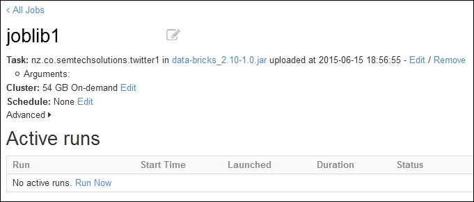
This tells me that the application library works. It connects to Twitter, creates a data stream, is able to filter the data into hash tags, and creates a temporary table using the data. So, having created a JAR library for Twitter data streaming, and proving that it works, I'm now able to load it onto the Databricks cloud. The following screenshot shows that a job has been created from the Databricks cloud jobs menu called joblib1. The Set Jar option has been used to upload the JAR library that was just created. The full package-based name to the twitter1 application object class has been specified.

The following screenshot shows the joblib1 job, which is ready to run. A Spark-based cluster will be created on demand, as soon as the job is executed using the Run Now option, under the Active runs section. No scheduling options have been specified, although the job can be defined to run at a given date and time.

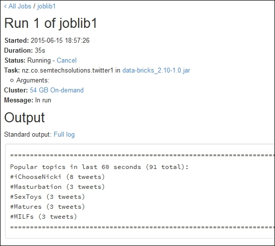
I selected the Run Now option to start the job run, as shown in the following screenshot. This shows that there is now an active run called Run 1 for this job. It has been running for six seconds. It was launched manually, and is pending while a on-demand cluster is created. By selecting the run name Run 1, I can see details about the job, especially the logged output.

The following screenshot shows an example of the output for Run 1 of joblib1. It shows the time started and duration, it also shows the running status and job details in terms of class and JAR file. It would have shown class parameters, but there were none in this case. It also shows the details of the 54 GB on-demand cluster. More importantly, it shows the list of the top five tweet hash tag values.

The following screenshot shows the same job run output window in the Databricks cloud instance. But this shows the output from the SQL count(*), showing the number of tweet hash tags in the current data stream tweet window from the temporary table.

So, this proves that I can create an application library locally, using Twitter-based Apache Spark streaming, and convert the data stream into data frames, and a temporary table. It shows that I can reduce costs by developing locally, and then port my library to my Databricks cloud. I am aware that I have neither visualized the temporary table, nor the DataFrame in this example, into a Databricks graph, but time scales did not allow me to do this. Also, another thing that I would have done, if I had time, would be to checkpoint, or periodically save the stream to file, in case of application failure. However, this topic is covered in Chapter 3, Apache Spark Streaming with an example, so you can take a look there if you are interested. In the next section, I will examine the Databricks REST API, which will allow better integration between your external applications, and your Databricks cloud instance.