
In the previous sections, you have been shown how to write Apache Spark graphx code in Scala to process the HDFS-based graph data. You have been able to execute the graph-based algorithms, such as PageRank, and triangle counting. However, this approach has a limitation. Spark does not have storage, and storing graph-based data in the flat files on HDFS does not allow you to manipulate it in its place of storage. For instance, if you had data stored in a relational database, you could use SQL to interrogate it in place. Databases such as Neo4j are graph databases. This means that their storage mechanisms and data access language act on graphs. In this section, I want to take a look at the work done on Mazerunner, created as a GraphX Neo4j processing prototype by Kenny Bastani.
The following figure describes the Mazerunner architecture. It shows that data in Neo4j is exported to HDFS, and processed by GraphX via a notification process. The GraphX data updates are then saved back to HDFS as a list of key value updates. These changes are then propagated to Neo4j to be stored. The algorithms in this prototype architecture are accessed via a Rest based HTTP URL, which will be shown later. The point here though, is that algorithms can be run via processing in graphx, but the data changes can be checked via Neo4j database cypher language queries. Kenny's work and further details can be found at: http://www.kennybastani.com/2014/11/using-apache-spark-and-neo4j-for-big.html.
This section will be dedicated to explaining the Mazerunner architecture, and will show, with the help of an example, how it can be used. This architecture provides a unique example of GraphX-based processing, coupled with graph-based storage.

The process for installing the Mazerunner example code is described via https://github.com/kbastani/neo4j-mazerunner.
I have used the 64 bit Linux Centos 6.5 machine hc1r1m1 for the install. The Mazerunner example uses the Docker tool, which creates virtual containers with a small foot print for running HDFS, Neo4j, and Mazerunner in this example. First, I must install Docker. I have done this, as follows, using the Linux root user via yum commands. The first command installs the docker-io module (the docker name was already used for CentOS 6.5 by another application):
[root@hc1r1m1 bin]# yum -y install docker-io
I needed to enable the public_ol6_latest repository, and install the device-mapper-event-libs package, as I found that my current lib-device-mapper, which I had installed, wasn't exporting the symbol Base that Docker needed. I executed the following commands as root:
[root@hc1r1m1 ~]# yum-config-manager --enable public_ol6_latest
[root@hc1r1m1 ~]# yum install device-mapper-event-libs
The actual error that I encountered was as follows:
/usr/bin/docker: relocation error: /usr/bin/docker: symbol dm_task_get_info_with_deferred_remove, version Base not defined in file libdevmapper.so.1.02 with link time reference
I can then check that Docker will run by checking the Docker version number with the following call:
[root@hc1r1m1 ~]# docker version
Client version: 1.4.1
Client API version: 1.16
Go version (client): go1.3.3
Git commit (client): 5bc2ff8/1.4.1
OS/Arch (client): linux/amd64
Server version: 1.4.1
Server API version: 1.16
Go version (server): go1.3.3
Git commit (server): 5bc2ff8/1.4.1
I can start the Linux docker service using the following service command. I can also force Docker to start on Linux server startup using the following chkconfig command:
[root@hc1r1m1 bin]# service docker start
[root@hc1r1m1 bin]# chkconfig docker on
The three Docker images (HDFS, Mazerunner, and Neo4j) can then be downloaded. They are large, so this may take some time:
[root@hc1r1m1 ~]# docker pull sequenceiq/hadoop-docker:2.4.1
Status: Downloaded newer image for sequenceiq/hadoop-docker:2.4.1

[root@hc1r1m1 ~]# docker pull kbastani/docker-neo4j:latest
Status: Downloaded newer image for kbastani/docker-neo4j:latest

[root@hc1r1m1 ~]# docker pull kbastani/neo4j-graph-analytics:latest
Status: Downloaded newer image for kbastani/neo4j-graph-analytics:latest
Once downloaded, the Docker containers can be started in the order; HDFS, Mazerunner, and then Neo4j. The default Neo4j movie database will be loaded and the Mazerunner algorithms run using this data. The HDFS container starts as follows:
[root@hc1r1m1 ~]# docker run -i -t --name hdfs sequenceiq/hadoop-docker:2.4.1 /etc/bootstrap.sh –bash

Starting sshd:                                [  OK  ]
Starting namenodes on [26d939395e84]
26d939395e84: starting namenode, logging to /usr/local/hadoop/logs/hadoop-root-namenode-26d939395e84.out
localhost: starting datanode, logging to /usr/local/hadoop/logs/hadoop-root-datanode-26d939395e84.out
Starting secondary namenodes [0.0.0.0]
0.0.0.0: starting secondarynamenode, logging to /usr/local/hadoop/logs/hadoop-root-secondarynamenode-26d939395e84.out
starting yarn daemons
starting resourcemanager, logging to /usr/local/hadoop/logs/yarn--resourcemanager-26d939395e84.out
localhost: starting nodemanager, logging to /usr/local/hadoop/logs/yarn-root-nodemanager-26d939395e84.out
The Mazerunner service container starts as follows:
[root@hc1r1m1 ~]# docker run -i -t --name mazerunner --link hdfs:hdfs kbastani/neo4j-graph-analytics
The output is long, so I will not include it all here, but you will see no errors. There also comes a line, which states that the install is waiting for messages:
[*] Waiting for messages. To exit press CTRL+C
In order to start the Neo4j container, I need the install to create a new Neo4j database for me, as this is a first time install. Otherwise on restart, I would just supply the path of the database directory. Using the link command, the Neo4j container is linked to the HDFS and Mazerunner containers:
[root@hc1r1m1 ~]# docker run -d -P -v /home/hadoop/neo4j/data:/opt/data --name graphdb --link mazerunner:mazerunner --link hdfs:hdfs kbastani/docker-neo4j
By checking the neo4j/data path, I can now see that a database directory, named graph.db has been created:
[root@hc1r1m1 data]# pwd
/home/hadoop/neo4j/data

[root@hc1r1m1 data]# ls
graph.db
I can then use the following docker inspect command, which the container-based IP address and the Docker-based Neo4j container is making available. The inspect command supplies me with the local IP address that I will need to access the Neo4j container. The curl command, along with the port number, which I know from Kenny's website, will default to 7474, shows me that the Rest interface is running:
[root@hc1r1m1 data]# docker inspect --format="{{.NetworkSettings.IPAddress}}" graphdb
172.17.0.5

[root@hc1r1m1 data]# curl  172.17.0.5:7474
{
  "management" : "http://172.17.0.5:7474/db/manage/",
  "data" : "http://172.17.0.5:7474/db/data/"
}
The rest of the work in this section will now be carried out using the Neo4j browser URL, which is as follows:
http://172.17.0.5:7474/browser.
This is a local, Docker-based IP address that will be accessible from the hc1r1m1 server. It will not be visible on the rest of the local intranet without further network configuration.
This will show the default Neo4j browser page. The Movie graph can be installed by following the movie link here, selecting the Cypher query, and executing it.
The data can then be interrogated using Cypher queries, which will be examined in more depth in the next chapter. The following figures are supplied along with their associated Cypher queries, in order to show that the data can be accessed as graphs that are displayed visually. The first graph shows a simple Person to Movie relationship, with the relationship details displayed on the connecting edges.

The second graph, provided as a visual example of the power of Neo4j, shows a far more complex cypher query, and resulting graph. This graph states that it contains 135 nodes and 180 relationships. These are relatively small numbers in processing terms, but it is clear that the graph is becoming complex.

The following figures show the Mazerunner example algorithms being called via an HTTP Rest URL. The call is defined by the algorithm to be called, and the attribute that it is going to act upon within the graph:
http://localhost:7474/service/mazerunner/analysis/{algorithm}/{attribute}.
So for instance, as the next section will show, this generic URL can be used to run the PageRank algorithm by setting algorithm=pagerank. The algorithm will operate on the follows relationship by setting attribute=FOLLOWS. The next section will show how each Mazerunner algorithm can be run along with an example of the Cypher output.
This section shows how the Mazerunner example algorithms may be run using the Rest based HTTP URL, which was shown in the last section. Many of these algorithms have already been examined, and coded in this chapter. Remember that the interesting thing occurring in this section is that data starts in Neo4j, it is processed on Spark with GraphX, and then is updated back into Neo4j. It looks simple, but there are underlying processes doing all of the work. In each example, the attribute that the algorithm has added to the graph is interrogated via a Cypher query. So, each example isn't so much about the query, but that the data update to Neo4j has occurred.
The first call shows the PageRank algorithm, and the PageRank attribute being added to the movie graph. As before, the PageRank algorithm gives a rank to each vertex, depending on how many edge connections it has. In this case, it is using the FOLLOWS relationship for processing.

The following image shows a screenshot of the PageRank algorithm result. The text at the top of the image (starting with MATCH) shows the cypher query, which proves that the PageRank property has been added to the graph.

The closeness algorithm attempts to determine the most important vertices in the graph. In this case, the closeness attribute has been added to the graph.

The following image shows a screenshot of the closeness algorithm result. The text at the top of the image (starting with MATCH) shows the Cypher query, which proves that the closeness_centrality property has been added to the graph. Note that an alias called closeness has been used in this Cypher query, to represent the closeness_centrality property, and so the output is more presentable.

The triangle_count algorithm has been used to count triangles associated with vertices. The FOLLOWS relationship has been used, and the triangle_count attribute has been added to the graph.

The following image shows a screenshot of the triangle algorithm result. The text at the top of the image (starting with MATCH) shows the cypher query, which proves that the triangle_count property has been added to the graph. Note that an alias called tcount has been used in this cypher query, to represent the triangle_count property, and so the output is more presentable.

The connected components algorithm is a measure of how many actual components exist in the graph data. For instance, the data might contain two subgraphs with no routes between them. In this case, the connected_components attribute has been added to the graph.
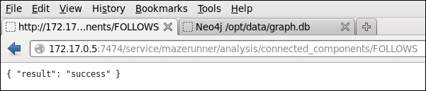
The following image shows a screenshot of the connected component algorithm result. The text at the top of the image (starting with MATCH) shows the cypher query, which proves that the connected_components property has been added to the graph. Note that an alias called ccomp has been used in this cypher query, to represent the connected_components property, and so the output is more presentable.

The strongly connected components algorithm is very similar to the connected components algorithm. Subgraphs are created from the graph data using the directional FOLLOWS relationship. Multiple subgraphs are created until all the graph components are used. These subgraphs form the strongly connected components. As seen here, a strongly_connected_components attribute has been added to the graph:

The following image shows a screenshot of the strongly connected component algorithm result. The text at the top of the image (starting with MATCH) shows the cypher query, which proves that the strongly_connected_components connected component property has been added to the graph. Note that an alias called sccomp has been used in this cypher query, to represent the strongly_connected_components property, and so the output is more presentable.
