The data we will be using is the match history data for the NBA for the 2013-2014 season. The website http://Basketball-Reference.com contains a significant number of resources and statistics collected from the NBA and other leagues. To download the dataset, perform the following steps:

This will download a CSV (short for Comma Separated Values) file containing the results of the 1,230 games in the regular season for the NBA.

CSV files are simply text files where each line contains a new row and each value is separated by a comma (hence the name). CSV files can be created manually by simply typing into a text editor and saving with a .csv extension. They can also be opened in any program that can read text files, but can also be opened in Excel as a spreadsheet.

We will load the file with the pandas (short for Python Data Analysis) library, which is an incredibly useful library for manipulating data. Python also contains a built-in library called csv that supports reading and writing CSV files. However, we will use pandas, which provides more powerful functions that we will use later in the chapter for creating new features.

$pip3 install pandas

The pandas library is a library for loading, managing, and manipulating data. It handles data structures behind-the-scenes and supports analysis methods, such as computing the mean.

When doing multiple data mining experiments, you will find that you write many of the same functions again and again, such as reading files and extracting features. Each time this reimplementation happens, you run the risk of introducing bugs. Using a high-class library such as pandas significantly reduces the amount of work needed to do these functions and also gives you more confidence in using well tested code.

Throughout this book, we will be using pandas quite significantly, introducing use cases as we go.

We can load the dataset using the read_csv function:

import pandas as pd
dataset = pd.read_csv(data_filename)

The result of this is a pandas Dataframe, and it has some useful functions that we will use later on. Looking at the resulting dataset, we can see some issues. Type the following and run the code to see the first five rows of the dataset:

dataset.ix[:5]

Here's the output:

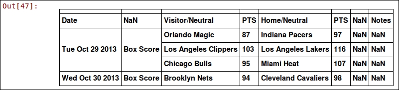
This is actually a usable dataset, but it contains some problems that we will fix up soon.

After looking at the output, we can see a number of problems:

These issues come from the data, and we could fix this by altering the data itself. However, in doing this, we could forget the steps we took or misapply them; that is, we can't replicate our results. As with the previous section where we used pipelines to track the transformations we made to a dataset, we will use pandas to apply transformations to the raw data itself.

The pandas.read_csv function has parameters to fix each of these issues, which we can specify when loading the file. We can also change the headings after loading the file, as shown in the following code:

dataset = pd.read_csv(data_filename, parse_dates=["Date"], skiprows=[0,])
dataset.columns = ["Date", "Score Type", "Visitor Team", "VisitorPts", "Home Team", "HomePts", "OT?", "Notes"]

The results have significantly improved, as we can see if we print out the resulting data frame:

dataset.ix[:5]

The output is as follows:

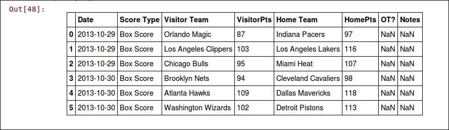
Even in well-compiled data sources such as this one, you need to make some adjustments. Different systems have different nuances, resulting in data files that are not quite compatible with each other.

Now that we have our dataset, we can compute a baseline. A baseline is an accuracy that indicates an easy way to get a good accuracy. Any data mining solution should beat this.

In each match, we have two teams: a home team and a visitor team. An obvious baseline, called the chance rate, is 50 percent. Choosing randomly will (over time) result in an accuracy of 50 percent.

We can now extract our features from this dataset by combining and comparing the existing data. First up, we need to specify our class value, which will give our classification algorithm something to compare against to see if its prediction is correct or not. This could be encoded in a number of ways; however, for this application, we will specify our class as 1 if the home team wins and 0 if the visitor team wins. In basketball, the team with the most points wins. So, while the data set doesn't specify who wins, we can compute it easily.

We can specify the data set by the following:

dataset["HomeWin"] = dataset["VisitorPts"] < dataset["HomePts"]

We then copy those values into a NumPy array to use later for our scikit-learn classifiers. There is not currently a clean integration between pandas and scikit-learn, but they work nicely together through the use of NumPy arrays. While we will use pandas to extract features, we will need to extract the values to use them with scikit-learn:

y_true = dataset["HomeWin"].values

The preceding array now holds our class values in a format that scikit-learn can read.

We can also start creating some features to use in our data mining. While sometimes we just throw the raw data into our classifier, we often need to derive continuous numerical or categorical features.

The first two features we want to create to help us predict which team will win are whether either of those two teams won their last game. This would roughly approximate which team is playing well.

We will compute this feature by iterating through the rows in order and recording which team won. When we get to a new row, we look up whether the team won the last time we saw them.

We first create a (default) dictionary to store the team's last result:

from collections import defaultdict 
won_last = defaultdict(int)

The key of this dictionary will be the team and the value will be whether they won their previous game. We can then iterate over all the rows and update the current row with the team's last result:

for index, row in dataset.iterrows():
    home_team = row["Home Team"]
    visitor_team = row["Visitor Team"]
    row["HomeLastWin"] = won_last[home_team]
    row["VisitorLastWin"] = won_last[visitor_team]
    dataset.ix[index] = row

Note that the preceding code relies on our dataset being in chronological order. Our dataset is in order; however, if you are using a dataset that is not in order, you will need to replace dataset.iterrows() with dataset.sort("Date").iterrows().

We then set our dictionary with the each team's result (from this row) for the next time we see these teams. The code is as follows:

    won_last[home_team] = row["HomeWin"]
    won_last[visitor_team] = not row["HomeWin"]

After the preceding code runs, we will have two new features: HomeLastWin and VisitorLastWin. We can have a look at the dataset. There isn't much point in looking at the first five games though. Due to the way our code runs, we didn't have data for them at that point. Therefore, until a team's second game of the season, we won't know their current form. We can instead look at different places in the list. The following code will show the 20th to the 25th games of the season:

dataset.ix[20:25]

Here's the output:

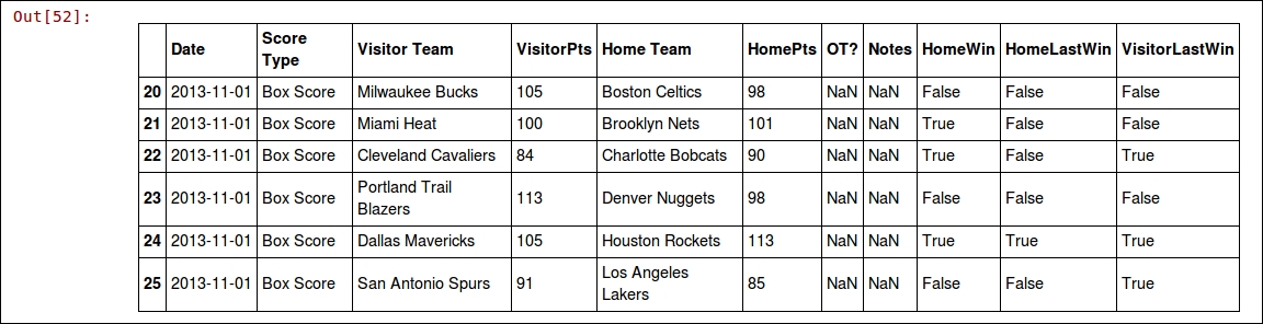
You can change those indices to look at other parts of the data, as there are over 1000 games in our dataset!

Currently, this gives a false value to all teams (including the previous year's champion!) when they are first seen. We could improve this feature using the previous year's data, but will not do that in this chapter.